2021 年 2 月
JOURNAL OF SOUTHWEST JIAOTONG UNIVERSITY
Feb. 2021
ISSN: 0258-2724 DOI:10.35741/issn.0258-2724.56.1.25
Research article
Environmental Sciences
A
SSESSMENT OF THE
I
MPACT OF
L
AND
C
OVER
T
YPE ON THE
W
ATER
Q
UALITY IN
L
AKE
T
ONDANO
U
SING A
SWAT
M
ODEL
用扑打模型评估土地覆盖类型对通达诺湖水质的影响。
Moh Sholichin*, Tri Budi Prayogo
Department of Water Resources Engineering, University of Brawijaya Malang, Indonesia, [email protected]
Received: November 27, 2020 ▪ Review: December 22, 2020 ▪ Accepted: January 26, 2021
This article is an open-access article distributed under the terms and conditions of the Creative Commons Attribution License (http://creativecommons.org/licenses/by/4.0)
Abstract
Lake Tondano is the largest natural lake in North Sulawesi, Indonesia, which functions as a provider of clean water, hydroelectric power, rice field irrigation, inland fisheries, and tourism. This research aims to determine the effect of land cover types from the Tondano watershed on the lake water quality. The Soil and Water Assessment Tool (SWAT) model was used to evaluate the rate of soil erosion and the pollutant load of various land types in the watershed during the last ten years. Rainfall data is obtained from two rainfall stations, namely Paleloan Station and Noonan Station. The model is calibrated and validated before being used for analysis. We use climatological data from 2014 to 2019. The process of the SWAT model calibration and validation was carried out with the statistical formulas of the coefficient of determination (R2) and Nash-Sutcliffe efficiency (NSE). The results show that the potential for
pollution load from the Tondao watershed is organic N of 0.039 kg/ha and organic P of 0.006 kg/ha coming from the agricultural land. The results of this study conclude that the fertility conditions of Lake Tondano are at the eutrophic level, where the pollutant inflow is collected in the lake waters, especially for the parameters of total N (1503697.44kg/year) and total P (144831.36kg/year). The SWAT simulation results show deviation between the modeling and field data collected with the value of R2 = 0.9303, and
the significant level ≤ 10.
Keywords: Pollutant, Water Quality, Soil and Water Assessment Tool (SWAT) Model
摘要通达诺湖是印度尼西亚北苏拉威西省最大的天然湖泊,可提供清洁水,水力发电,稻田灌溉 ,内陆渔业和旅游业。本研究旨在确定通多诺流域的土地覆盖类型对湖泊水质的影响。扑打模型 用于评估近十年来流域内各种土地类型的土壤侵蚀速率和污染物负荷。降雨数据是从两个降雨站 (即帕洛洛安站和努南站)获得的。在用于分析之前,先对模型进行校准和验证。我们使用 2014
年至 2019 年的气候数据。使用确定系数(R2)和纳什-苏特克利夫效率(NSE)的统计公式进行了 扑打模型的校准和验证过程。结果表明,通达河流域的污染负荷潜力是来自农田的有机氮为 0.039 公斤/公顷,有机磷为 0.006 公斤/公顷。研究结果表明,通达诺湖的肥力条件处于富营养 化水平,其中污染物流入湖水,特别是对于总氮(1503697.44 公斤/年)和总磷(144831.36 公斤 /年)。扑打仿真结果表明建模与实地数据之间存在偏差,R2 = 0.9303,显着水平≤10。 关键词: 污染物,水质,水土评估工具
I.
I
NTRODUCTIONNatural ecosystems already provide important ecosystem factors needed by humans (for example, carbon sequestration, land retention, biodiversity, climate regulation, and recreation) to sustain social and economic development [1, 2]. Decreasing the concentration of sediment and essential nutrients in freshwater ecosystems is very influential on natural processes and processes managed by humans [3].
Under the Law No. 7 of 2004 concerning Water Resources, lake or situ management consists of three main components, conservation, utilization, and control over the destructive force of water. Government Regulation Number 82 of 2001 states that efforts to manage water quality
in rivers and lakes include determining the capacity of rivers or lakes, determining the designation of rivers or lakes, accompanied by water quality standards.
From time to time, Lake Tondano is getting shallower, and water hyacinths overgrow some its areas. There are many fish cages in several places on the edge of Lake Tondano, where the leftover fish food becomes waste that pollutes the lake water.
The function of Lake Tondano for the community is very important, so it is necessary to protect the water quality. Poor water quality in rivers that enter the lake can cause decline in water quality, resulting in eutrophic waters, so it is feared that the lake will be heavily polluted.
The second purpose of this study was to determine the distribution pattern and risk classification of the eutrophication hazard in Lake Tondano; find out the carrying capacity of the lake against pollutant loads that cause the risk of lake eutrophication; calculate and map the watershed areas that have the potential to be a source of the largest pollutant inflow into Lake Tondano based on various aspects such as the area and density of villages, paddy fields, plantations and wasteland, industrial activities and fisheries; create a system and policy for
managing and handling waste that is appropriate for the condition of waters in Lake Tondano and the watershed.
II. M
ETHODOLOGYA. The Research Site
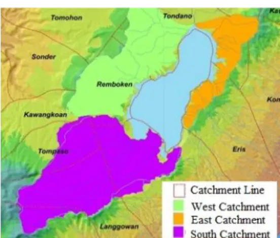
The study area lies on the geographic route between1°27'34,82" - 1°01'51,37" North Latitude and 124°32'05" - 125°03'46,33" East Longitude. The study area is located in the southern part of Manado City, the capital city of North Sulawesi Province. Physiographically, the area in the shape of an area covers an area of about 54,755 ha. Lake Tondano, which has an area of 4,638 ha, is located in the southern part of the Study Area. Administratively, the study area is part of the Minahasa Regency, which consists of 11 Districts and 146 Villages, and the City of Manado, which consists of 4 Districts in the North Sulawesi Province.
Figure 1. The research site
The water of Lake Tondano is used as drinking water for residents, and also for irrigation, hydroelectric power, inland fisheries, and tourism. The condition of many lakes in Indonesia has decreased due to sediments and water pollution [4]. The study area consists of four kinds of geological formations: Lacustrine and Fluviatile (Qs) deposits, young volcanic rocks (Qv), Tuff Tondano (Qtv), and old volcanic rocks (TMV). Figure 2 shows the topography of
L
o k a s i
P
the Lake Tondano area, while Figure 3 shows the Lake Tondano watershed.
Figure 2. DEM at the research site
Figure 3. The research site catchment
B. The SWAT Model
The Soil and Water Assessment Tool (SWAT) is a time-continuous and semi-spatially distributed model developed to simulate the impact of management decisions on water, sediment, and agricultural chemical yields in river basins concerning soil, land use, and management practices [5-7]. The model represents the large-scale spatial variability of soil, land use, and management practices by discrediting the catchment into sub-units using a two-step approach [8].
A topographic discretization is done by dividing the catchment into sub-units based on a minimum drainage area. Then, each sub-catchment is divided into one or several homogeneous hydrological response units (HRUs) obtained by overlaying the soil and land use maps. The HRUs have no exact geographical location and no spatial link to each other; they are associated only to a sub-basin. The response of each HRU in terms of water, sediment, nutrient, and pesticide transformations and losses are determined, then aggregated at the sub-basin level and routed to the catchment outlet through the channel network [8].
Based on the theoretical documentation of SWAT, major equations are introduced as follows:
(i) Soil Water. The hydrologic cycle as simulated by SWAT is based on the water balance equation [9]:
𝑆𝑊𝑡 = 𝑆𝑊0+ ∑𝑡𝑖=1(𝑅𝑑𝑎𝑦− 𝑄𝑠𝑢𝑟𝑓− 𝐸0−
𝑤𝑠𝑒𝑒𝑝− 𝑄𝑔𝑤) (1)
where t is the time (days), SWt is the final soil
water content (mm H2O), SW0 is the initial soil
water content (mm H2O), Rday, Qsurf, Ea, wseep,
and Qgw are the daily amounts of precipitation,
runoff, evapotranspiration, percolation and return flow, respectively.
(ii) Surface Runoff. SWAT uses mainly the SCS curve number procedure for estimating the surface runoff. The SCS curve number equation is 𝑄𝑠𝑢𝑟𝑓 = (𝑅𝑑𝑎𝑦−0.2𝑆) 2 (𝑅𝑑𝑎𝑦+0.8𝑆) ; 𝑆 = 25.4 ( 1000 𝐶𝑁 − 10) (2) where Q
surf is the accumulated runoff or rainfall
excess, R
day is the rainfall depth for the day, S is
the retention parameter, and CN is the curve number for the day.
(iii) Nutrient Transport. Organic N attached to soil particles may be transported by surface runoff to the main channel. This form of nitrogen is associated with the sediment loading from the HRU, and changes in sediment loading will be reflected in the organic nitrogen loading. The amount of organic nitrogen transported with sediment to the stream is calculated with the following equation: 𝑜𝑟𝑔𝑁𝑠𝑢𝑟𝑓 = 0.001. 𝑐𝑜𝑛𝑐𝑜𝑟𝑔𝑁. 𝑠𝑒𝑑 𝑎𝑟𝑒𝑎ℎ𝑟𝑢. 𝜀𝑁𝑠𝑒𝑑 (3) where orgN
surf is the amount of organic nitrogen
transported to the main channel in surface runoff,
conc
orgN is the concentration of organic nitrogen
in the top 10mm, sed is the sediment yield on a given day, area
hruis the HRU area, and εN:sed is
the nitrogen enrichment ratio.
Because of the low mobility of phosphorus solution, surface runoff will only partially interact with the P solution stored in the top 10mm of soil. The amount of P solution transported in surface runoff is as follows:
𝑃𝑠𝑢𝑟𝑓 =
𝑃𝑠𝑜𝑙𝑢𝑡𝑖𝑜𝑛,𝑠𝑢𝑟𝑓.𝑄𝑠𝑢𝑟𝑓
𝜌𝑏.𝑑𝑒𝑝𝑡ℎ𝑠𝑢𝑟𝑓.𝑘𝑑,𝑠𝑢𝑟𝑓 (4)
where Psurfaceis the amount of soluble phosphorus lost in the surface runoff, Psolution, surface is the amount of solution phosphorus in the top 10mm,
Q
surfaceis the same as stated above, ρb is the bulk
density of the top 10mm, depth
surface is the depth
of the "surface" layer (10mm), and k
d, surface is the
phosphorus soil partitioning coefficient.
(iv) Nutrient Cycles. Humus mineralization of nitrogen: Nitrogen is allowed to move between the active and stable organic pools in the humus fraction. The amount of nitrogen transferred from one pool to the other is calculated as:
𝑁𝑡𝑚𝑠,𝑙𝑦= 𝛽𝑡𝑚𝑠. 𝑜𝑟𝑔𝑁𝑎𝑐𝑡,𝑙𝑦. ( 1
𝑓𝑟𝑎𝑐𝑡.𝑁− 1) −
𝑜𝑟𝑔𝑁𝑠𝑡𝑎,𝑙𝑦 (5)
where N
trns,ly is the amount of nitrogen transferred
between the active and stable organic pools (kg N/ha), β
trns is the rate constant (1×10
−5
), orgN
act,ly
is the amount of nitrogen in the active organic pool (kg N/ha), fr
actN is the fraction of humic
nitrogen in the active pool (0.02), and orgsta,ly is the amount of nitrogen in the stable organic pool (kg N/ha).
Ammonium is converted via nitrification and volatilization:
𝑁𝑛𝑖𝑡,𝑣𝑜𝑙,𝑙𝑦= 𝑁𝐻4,𝑙𝑦− (1 − 𝑒𝑥𝑝[−𝜂𝑛𝑖𝑡,𝑙𝑦−
𝜂𝑣𝑜𝑙,𝑙𝑦]) (6)
where N
nit/vol,ly is the amount of ammonium
converted via nitrification and volatilization in layer ly (kg N/ha), NH
4ly is the amount of
ammonium in layer ly (kg N/ha), η
nit,ly is the
nitrification regulator, and η
vol,ly is the
volatilization regulator.
Denitrification: SWAT determines the amount of nitrate lost to denitrification by the following equations: 𝑁𝑑𝑒𝑛𝑖𝑡,𝑙𝑦 = 𝑁𝑂3𝑙𝑦. (1 − 𝑒𝑥𝑝[−1.4𝛾𝑡𝑚𝑝,𝑙𝑦. 𝑜𝑟𝑔𝐶𝑙𝑦]), if →𝛾𝑠𝑤,𝑙𝑦≥ 0.95 (7) 𝑁𝑑𝑒𝑛𝑖𝑡,𝑙𝑦 = 0.0if →𝛾𝑠𝑤,𝑙𝑦 ≤ 0.95 (8) where N
denit,ly is the amount of nitrogen lost to
denitrification (kg N/ha), NO
3ly is the amount of
nitrate in layer ly (kg N/ha), γ
tmp,ly is the nutrient
cycling temperature factor for layer ly, γ
sw,ly is the
nutrient cycling water factor for layer ly, orgC
lyis
the amount of organic carbon in the layer (%). Calculation of the movement of phosphorus between the solution and the active mineral pool using the equilibration equation:
𝑃𝑠𝑜𝑙,𝑎𝑐𝑡,𝑙𝑦= 𝑃𝑠𝑜𝑙𝑢𝑡𝑖𝑜𝑛,𝑙𝑦 − 𝑚𝑖𝑛 𝑃𝑎𝑐𝑡,𝑙𝑦. ( 𝑃𝑎𝑖 1 − 𝑃𝑎𝑖) i 𝑃𝑠𝑜𝑙𝑢𝑡𝑖𝑜𝑛,𝑙𝑦 > 𝑚𝑖𝑛 𝑃𝑎𝑐𝑡,𝑙𝑦. ( 𝑃𝑎𝑖 1−𝑃𝑎𝑖) (9) 𝑃𝑠𝑜𝑙,𝑎𝑐𝑡,𝑙𝑦= 0.1 [𝑃𝑠𝑜𝑙𝑢𝑡𝑖𝑜𝑛,𝑙𝑦 − 𝑚𝑖𝑛 𝑃𝑎𝑐𝑡,𝑙𝑦. ( 𝑃𝑎𝑖 1 − 𝑃𝑎𝑖)] If 𝑃𝑠𝑜𝑙𝑢𝑡𝑖𝑜𝑛,𝑙𝑦< 𝑚𝑖𝑛 𝑃𝑎𝑐𝑡,𝑙𝑦. ( 𝑃𝑎𝑖 1−𝑃𝑎𝑖) (10)
where Psol/act,ly is the amount of phosphorus transferred between the soluble and active mineral pools (kg P/ha), Psolution,ly is the amount of phosphorus in solution (kg P/ha), minPact,ly is the amount of phosphorus in the active mineral pool (kg P/ha), and Pai is the phosphorus
availability index.
C. Nutrient Load
The regression model was used to predict constituent loads as a function of runoff volume for the study period. The linear relationships developed were used to estimate a representative concentration for days not sampled, using the mean daily flow as input to the linear regression equation.
The species annual load was calculated as the summation of daily load, expressed by the equation:
𝐷𝑎𝑖𝑙𝑦𝐿𝑜𝑎𝑑 =
∫ 𝑄𝑖𝑥𝐶𝑖𝑑𝑡 (11)
where Qi represents the mean daily hydrologic
flow (m3/sec), and C
i represents the mean daily
species concentrations. The daily load is expressed in kg/day, annual load in kg/year, and annual yield is expressed as kg/ha/year.
𝐴𝑛𝑛𝑢𝑎𝑙𝐿𝑜𝑎𝑑 = ∑365𝐷𝑎𝑖𝑙𝑦𝐿𝑜𝑎𝑑 𝑖=1 (12) 𝐴𝑛𝑛𝑢𝑎𝑙𝑌𝑖𝑒𝑙𝑑 = ∑ ( 𝐴𝑛𝑛𝑢𝑎𝑙𝐿𝑜𝑎𝑑 𝑠𝑢𝑏_𝑤𝑎𝑡𝑒𝑟𝑠ℎ𝑒𝑑𝑎_𝑎𝑟𝑒𝑎) 365 𝑖=1 (13)
In this research, statistical software was used to analyze each parameter. These statistical analyses are an important step in determining if water quality criteria have exceedingly degraded in the study area. To calculate the annual loads of nutrients, linear regression equations (mean daily flow vs. constituent load) were generated and evaluated using the coefficient of determination (R2) and the statistical (P<0.05) value.
A 50 × 50m raster digital elevation map was available. The elevation data were processed using the SWAT-ArcView interface, subdividing the catchment into 55 sub-basins. The DEM was used to estimate all routing characteristics kept unchanged for the remainder of the study. The dominant soil and land use were determined, resulting in one HRU, i.e., one unique soil type and land use combination per sub-basin. Each sub-basin was assigned a runoff curve number based on the hydrological soil group, cover type, and management practices, as described previously. Sixty-seven rainfall stations provided daily rainfall measurements for the 1990–2006 periods. Daily measurements of maximum, minimum, and average air temperature were available for six stations [8].
The actual management practices included fertilizer applications in planting paddy season. The average fertilizer application rate is around 150kg/ha for nitrogen and 100kg/ha of phosphorus. The variables used during the calibration-validation exercise included monthly water flow, suspended sediment, nitrate, and ortho-phosphorus concentrations covering the 1993–2007 period and were provided by the Directorate of Agriculture of Indonesia Government.
D. Model Calibration
Model performance was assessed by the coefficient of determination (R2), root means
square error (RMSE), and the Nash–Sutcliffe coefficient (EN–S) Nash & Sutcliffe 1970). RMSE
and EN–S were calculated as:
𝑅𝑀𝑆𝐸 = √1 𝑛∑ (𝑄𝑜− 𝑄𝑠) 2 𝑛 𝑖−1 (14) 𝐸𝑁−𝑆= 1 − ∑𝑛𝑖−1(𝑄𝑜−𝑄𝑠)2 ∑𝑛𝑖−1(𝑄𝑜−𝑄𝐴𝑉)2 (15)
where Qo and Qs were the observed and
simulated values, respectively, and QAV was the
average of observed values.
E. Pollutant Transport Mechanism
In this study area, pollutant transport mechanism is divided into three parts of the subject that must be completed sequentially and systematically, namely:
a. a pattern of the potential spread of pollutants in the watershed area of Lake Tondano
b. spreading pattern of pollutants in rivers, and
c. tributaries that estuary into Lake Tondano
(16) where C is concentration of water quality parameters (mg/L); Ux, Uy, Uz are longitudinal, lateral, and vertical velocities (m/day); Ex, Ey, Ez are longitudinal, lateral and vertical velocity coefficients of spread (m2/day); S
L is a total level
of distributed, and direct load (gr/m3-day); S
B is a
number of boundary load levels, namely upstream, downstream, aquatic plants, and atmosphere (gr/m3-day); S
K is a number of levels
of kinetic transformation (gr/m3-day).
IV. R
ESULTS ANDD
ISCUSSIONA. Model Performance
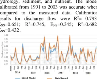
Model calibration and validation are necessary and critical steps in any model application [10]. Model validation is, in reality, an extension of the calibration process. Its purpose is to assure that the calibration model properly assesses all the variables and conditions which can affect model results and demonstrate the ability to predict field observations for periods separate from the calibration effort. The SWAT model was calibrated in three location stations. Calibration of the model had three steps: hydrology, sediment, and nutrient. The model calibrated from 1991 to 2003 was accurate when compared to the measured data. Calibration results for discharge flow were R2= 0.793,
ENS=0.651; R2=0.745, ENS=0.345; R2=0.682,
ENS=0.432 .
Figure 4. The research site catchment. Comparison and deviation of model results and AWLR discharge record
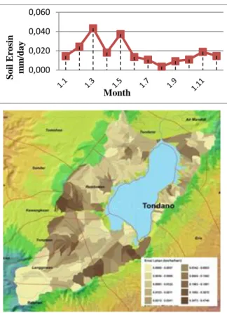
B. Soil Erosion
The results of the SWAT Running model show that land erosion is more dominant in the western and southern lands, where the average rate of soil erosion in the Lake Tondano catchment is 0.05 ton/ha/day or 17.88 ton/ha/year, in comparison to the maximum average soil erosion in the catchment is 0.12 ton/ha/day in November (see Figure 5).
Figure 5. Soil erosion distribution
C. Organic N Pollutant Load
There are three main forms of nitrogen in the soil, organic N related to humus, mineral N from soil colloids, and mineral N in solution. Nitrogen is removed from the soil by plant infiltration, water drainage, evaporation, and erosion. Nitrogen in the soil is carried into rivers through surface runoff. The amount of rain, soil type, land management results (fertilization, plowing, irrigation, etc.), surface runoff, and erosion impact the amount of nitrogen transport that occurs on land [11].
In the western area, the distribution of organic pollutants N is 13.87 kg/ha/year, with a maximum average of 0.113 kg N/ha/ day in November. In the East area of Lake Tondano, a catchment of 9.125 kg N/ha/year, with a maximum average of 0.062 kg N/ha/day in March. Moreover, on the land to the South, the organic pollutant load of N in the land is 20.81 kg/ha/year, and a maximum average of 0.101 kg N/ha/day in May.
Figure 6. Organic N load distribution
D. Organic P Pollutant Load
There are three main phosphorus forms in soil: organic P related to humus, the soluble form of phosphorus minerals (soluble P), and mineral P in soil solution (soluble P).
On average, in the western part of the Lake Tondano watershed, the organic pollutant load was 1.825 kg P/ha/year, with a maximum average incidence of 0.014 kg P/ha/day in November. In the eastern watershed area of Lake Tondano, it is 1.095 kg P/ha /year, with a maximum average of 0.008 kg P/ha/day in March. In the southern part of the Lake Tondano watershed, the organic P pollutant load on the land is 1.46 kg /ha/year, with a maximum average incidence of 0.008 kg P/ha/day also in March (see Figure 7).
Figure 7. Organic P load distribution
E. Sediment Inflow to the Lake
The total average sediment of Lake Tondano is 513.53 tons/day where the sediment sources from each of the Lake Tondano watershed areas are:
- the western part of the total sediment that enters Lake Tondano accounts for 337.24 tons/day with maximum sediment of 408.98 tons/day, and minimum 173.45 tons/day,
0,000 0,020 0,040 0,060 S o il Er o sin m m /d a y Month
- the eastern part amounts to 60.02 tons of sediment per day with maximum sediment of 138.58 tons/day and minimum 13.33 tons/day, and
- the southern part with sediment inflow maximum 233.99 tons/day, and minimum 33.93 tons/day.
F. Pollutant Distribution in Lake Tondano
To analyze the pollution load that enters the water bodies of Lake Tondano, the WASP Program is used to detect the distribution of pollutants in the lake inundation area. The Water Quality Analysis Simulation Program (WASP) enhances the original WASP [12]. This model helps users interpret and predict water quality responses to natural phenomena and human-made pollution for various pollution management decisions.
Input and division of WASP modeling segments for this study is shown in Figure 8. The area of Lake Tondano waters is divided into 33 total segments. The WASP model also carried out a calibration process with satisfactory results R2 = 9.86% degree of deviation.
The results of running the WASP model can be seen in Figures 9 and 10 for pollutant N and pollutant P, respectively.
Based on the nutrient concentrations of organic N and organic P, the level of eutrophication in the aquatic environment can be classified as oligotrophic, mesotrophic, eutrophic, and hypereutrophic.
Figure 8. Map for modeling segment divisions
Figure 9. Pollutants distribution pattern for organic N in Lake Tondano
Figure 10. Pollutants distribution pattern for organic P in Lake Tondano
The oligotrophic environment is characterized by clear water, little suspended organic matter or sediment, and low primary production (phytoplankton growth). Mesotrophic environments have higher nutrient input and moderate phytoplankton growth rates. Eutrophic environments have very high-nutrient-high-nutrient concentrations, and biological productivity occurs, such as water hyacinths that begin to thrive.
The carrying capacity of Lake Tondano is influenced by the pattern of elevation of lake water during the dry season and the rainy season (see Tables 1 and 2). This is a resume of rising water in the lake water and its effect on the water pollution load.
It can be concluded that in the waters of Lake Tondano, the total pollutant load of total N and total P is in eutrophic alert status so that Lake Tondano is no longer able to accommodate the pollutant load that enters the lake. Handling efforts should be divided into two, namely: a) Handling in the watershed: Arrangement of the watershed area and inhibiting rate of transport of river pollutants to Lake Tondano by placing the check dam, and wetland in the river upstream of
Lake Tondano, controlling the mining of class C minerals in the Tondano watershed and controlling villages. b) Handling in water: controlling chemical fertilizers and pesticides and controlling floating net cages, minimizing erosion, sedimentation, and regulation of water systems in rivers and lakes, restoring water quality due to disposal of domestic waste, and controlling eutrophication and water weeds.
IV. C
ONCLUSIONSBased on the research results obtained, the following conclusions are drawn:
1. The distribution pattern of pollutant load of water body of Lake Tondano was influenced by the source of inflow from the rivers and its tributaries. Based on the discussion results, the current source of the Lake Tondano inflow has experienced a eutrophic alert status.
2. Based on the trophic class, the lake is currently unable to accommodate the incoming pollutant load; it has exceeded the mesotrophic class limit.
3. As a result of land use in the Lake Tondano watershed, the Lake Tondano watershed area has a high potential to produce pollutants that will enter to waters, which dominant N pollutant based in the upstream watershed area,
while P pollutant is evenly distributed from the right and left watershed areas, namely:
a. For the watershed upstream of Lake Tondano, the average value of organic N pollutants is 0.038 kg N/ha/day, the average value of organic P pollutants is 0.005 kg P/ha/day, the average value of organic NO3 pollutants is
0.002 kg N/ha/day, the average value of mineral P pollutants is 0.002 kg P/ha/day, and the average value of soil dissolved phosphorus pollutants is 0.00013 kg P/ha/day.
b. For the right-hand watershed of Lake Tondano, the average value of organic N pollutants is 0.025 kg N/ha/day, the average value of organic P pollutants is 0.003 kg P/ha/day, the average value of organic NO3 pollutants is
0.001 kg N/ha/day, the average value of mineral P pollutants is 0.001 kg P/ha/day, and the average value of soil dissolved phosphorus pollutants is 0,0001 kg P/ha/day.
For the left-hand watershed of Lake Tondano, the average value of organic N pollutants is 0,057 kg N/ha/day, the average value of organic P pollutants is 0.004 kg P/ha/day, the average value of organic NO3 pollutants is 0.051 kg N/ha/day,
the average value of mineral P pollutants is 0.001 kg P/ha/day, and the average value of soil.
Table 1.
Fertility quality standard total N capacity of lake or reservoir
Total N Oligotrophic
Z (Average Depth) ρ N std (mg/m3) R' x R L (mg/m2year) L (kg/m2year)
14.54 0.29 650.000 0.72 0.55 0.872 21368.55 0.0214
Mesotrophic
14.54 0.29 750.000 0.72 0.55 0.872 24656.02 0.0247
Eutrophic
14.54 0.29 1900.000 0.72 0.55 0.872 62461.93 0.0625
Note: P std = Guidelines for Lake Ecosystem Management, KLH, 2009
Table 2.
Fertility quality standard total P capacity of lake or reservoir
Total P Oligotrophic
Z (Average Depth) ρ Pstd (mg/m3) R' x R L (mg/m2year) L (kg/m2year)
14.54 0.29 10.00 0.71 0.55 0.872 328.75 0.0003
Mesotrophic
14.54 0.29 30.00 0.71 0.55 0.872 986.24 0.0010
Eutrophic
14.54 0.29 100.00 0.71 0.55 0.872 3287.47 0.0033
Note: P std = Guidelines for Lake Ecosystem Management, KLH, 2009