芝浦工業大学学術リポジトリ

(1)

Evaluation of Trans-femoral

Prosthesis Function Using Finite

Element Analysis

A DISSERTATION SUBMITTED TO THE

GRADUATE SCHOOL OF ENGINEERING AND SCIENCE OF SHIBAURA INSTITUTE OF TECHNOLOGY

by

LE VAN TUAN

IN PARTIAL FULFILLMENT OF THE REQUIREMENTS FOR THE DEGREE OF

DOCTOR OF ENGINEERING

(2)

(3)

Acknowledgments

I owe a deep sense of gratitude to all kindnesses and supports for my studies. Like once said that no one succeeds all by themselves, the work would not have been completed without the help of many individuals.

First and foremost, I would like to send my deepest appreciation to my family for their spiritual support, which motivates and encourages me to accomplish the research successfully. Moreover, those achievements of mine could not be attained without the presence of my wife, who has always been by my side and has given me strength to overcome the difficulties during these four years of hard working.

I would like to express my gratitude to my supervisor, Professor Aki-hiko Hanafusa, for his research orientation from the very beginning of my study, the guidelines, valuable advice, throughout the time of the research as well as his enthusiastic supervision and encouragement for the successful completion of this dissertation.

I would also like to thank Prof. Shinichiroh Yamamoto, Prof. Kengo Ohnishi, Prof. Hiroshi Otsuka, and Prof. Yukio Agarie for their per-ceptive comments on the thesis in view of the fact that these comments not only led to the enhancement of my work but also suggested new tendencies for the research development.

(4)

kind help and endless support. In addition, I am very grateful to my Japanese friends who have willingly helped me to become familiar with a new place, way of life and language here in Japan. Thanks to their moral support, I had more time to work at a high level without being distracted.

Furthermore, immeasurable appreciation is extended to all members of prosthesis and orthosis group for providing me a chance to get the use of prosthesis devices, do experiments. Last but not least, I am very grateful to my kind friends and colleagues who are one way or another shared their support and understanding spirit, thank you all.

Saitama, September, 2017

(5)

Abstract

A transfemoral prosthesis is an artificial limb that replaces a leg miss-ing above the knee. The transfemoral amputee must deal with in-creased energy consumption for ambulation, balance, and stability; a more complicated prosthetic device; difficulty rising from sitting to standing. Transfemoral amputees can have a very difficult time regaining normal movement. A transfemoral prosthesis includes the following components: a socket, knee part, shank, ankle foor and sus-pension mechanism. For the transfemoral amputee to achieve the best possible outcome, it is necessary for the prosthetist to understand the prosthetic components and how they work. In this study, the author refers to the understandings about features of transfemoral prosthe-sis, methods and engineerings used in evaluated and manufactured transfemoral prosthesis. In this study, the author present a method for evaluation the functions of transfemoral prosthesis part by finite element method. The results of this study suggest that this method can used by the designer and prosthetist for design and choose the best comfortable prosthesis for the patient and reduce time for train-ing before use the transfemoral prosthesis. This study includes six chapters were structured as follows.

Chapter 1: Introduction

(6)

prosthesis are summarized to high light the necessary of this study. Finally, the contributes and the abstract of all chapters provides a panoramic view of the entire of study.

Chapter 2: Technical Background and Literature Review

This chapter presents an overview of finite element analysis, multi-body simulation and review the related studies. In the first section, the fundamental of finite element analysis and multibody simulation are briefly presented. This part provides the most important concepts and theory for the whole work. In the next section, the previous study are reviewed. Some prevailing results of studies are also introduced to clarify the novelty of the contributions in this work.

Chapter 3: Evaluation interface pressure on surface of residual limb in standing posture

(7)

Chapter 4: Transfemoral Gait Cycle Analysis and Evaluation Inter-face Pressure On SurInter-face Of Residual Limb In Gait Cycle

This chapter present the analysis of kinematic transfemoral gait and the method for evaluation interface pressure on surface of residual limb in gait cycle. There are the different between the human normal gait and transfermoral gait. Even, there are very different of individ-ual transfemoral patient. Understand the properties of gait pathology is very important in rehabiliation program. The multibody simulation method was used for analysis the gait cycle of transfemoral prosthesis. After that a method for computation the interface pressure between socket and residual limb during walking of patient with some of the limitation movement of residual limb and socket was presented. The shape of socket was assumed the same with the residual limb. The kinematics data of residual limb with prosthesis were observed by mo-tion analysis system. The total model includes residual limb and all components of transfemoral socket were modeled in real size. The experiment was conducted to measure the value of pressure between socket and residual limb. The results of two methods were compared and disscused.

Chapter 5: Estimation of the ground reaction force and pressure be-neath the foot prosthesis during the gait of transfemoral patients

(8)

similar data between the simulation and the measurement. A corre-lation coefficient of 0.91 between them denotes their correspondence. The reaction force at knee joint, distribution of beneath pressure of foot prosthesis were included in results and discussion. These results can be used for prosthesis design and optimization; they can assist the prosthetist in selecting a comfortable prosthesis for the patient and in improving the rehabilitation training.

Chapter 6: Conclusion and future work

(9)

Nomenclature

Roman Symbols

3D Three Dimension AD Anterior Distal

AKA Above Knee Amputation AP Anterior Proximal

BKA Below Knee Amputation CAD Computer Aid Design

CAT-CAM Contour Adducted Trochanteric Controlled Aligment Method COP Center Of Pressure

FE Finte Element

FEA Finte Element Analysis FEM Finte Element Method GRF Ground Reaction Force HFE high frequency events

(10)

NOMENCLATURE

LP Lateral Proximal

MCCT Manual Compression Casting Technique MD Medial Distal

MP Medial Proximal

MRI magnetic resonance image

NRCD National Disabled Persons Rehabilitation Center PD Posterior Distal

PP Posterior Proximal

SACH Solid Ankle Cushion Heel TSB Total Surface Bearing

UCLA University of California Los Angeles UK United of Kingdom

US United State

(11)

List of Figures

1.1 Amputation levels (NRCD - Japan) . . . 4

1.2 Main components of the lower limb prosthesis (NRCD Japan). Hip prosthesis (left); Transfemoral prosthesis (middle) and Transtibial prosthesis (right) . . . 6

1.3 Prosthetic socket made of lamination resin (Ottobock)) . . . 7

1.4 The UCLA socket type and MCCT socket type. Made by prof. Agarie laboratory. . . 8

1.5 Knee joint system (Otto Bock) . . . 10

1.6 The Triton family of feet (Otto Bock) . . . 12

2.1 Divide the domain into a number of small, simple elements (MIT web) . . . 21

2.2 Different 1D, 2D and 3D basic elements . . . 23

2.3 FEA Preprocessing (simplan.de) . . . 26

2.4 FEA Postprocessing (simplan.de) . . . 26

2.5 Wayne State Human Body Model - II . . . 27

2.6 Multibody Simulation with Simmechanics (Matworks Inc). . . 28

2.7 Example of Simmechanics Block Diagram (Matworks Inc). . . 30

2.8 Simple models of human gait. (a) Inverted pendulum model [50]. (b) 2D passive walking [43]. (c) Cornell 3D passive biped with arms [33]. . . 34

(17)

LIST OF FIGURES

2.10 Volunteer protected by kneepads falling from gait onto one knee. B: Numerical model of the subject with the coordinate system, where the loads are simulated [27]. . . 35 2.11 Ground reaction force (spartascience.com) . . . 36 2.12 Distribution of the plantar pressures [32]. . . 37 3.1 Profile at the cross section from distal end of (a) residual limb, (b)

UCLA socket, and (c) MCCT socket at 180 mm . . . 43 3.2 Posture of patient (a), MRI process (b), MRI image (c). . . 44 3.3 3D model of parts of residual limb. (a. Skin; b. Fat; c. Muscle; d.

Bone). . . 45 3.4 The FE model of residual limb in case of different shape with

MCCT socket (a); same shape with MCCT socket (b) and the socket (c). . . 46 3.5 Experiment diagram . . . 49 3.6 The position of eight sensors on socket . . . 50 3.7 Comparison of interface pressure between experiment and

simula-tion in the case of the shape of the socket and residual limb are the same and different. . . 53 3.8 The scatter diagram shows the relation between experimental

re-sults and two cases of simulation rere-sults. . . 54 3.9 The value of pressure at sensors location in the experiment and

simulation in case of MCCT (a) and UCLA (b) socket with 50 percent body weight. . . 57 3.10 The value of pressure at sensors location in the experiment and

simulation in case of MCCT (a) and UCLA (b) socket with 50 percent body weight. . . 58 3.11 Distribution of interface pressure (Unit: MPa). Anterior (left side)

(18)

LIST OF FIGURES

4.2 Divisions of Gait Cycle. . . 65

4.3 The diagram demonstrates this division of gait cycle. . . 67

4.4 Experiment with Mac3D System. . . 70

4.5 Schema movement of lower limb with prosthesis (mm). . . 71

4.6 Position of markers and angles on lower limb. . . 72

4.7 Rotation Angle at Hip and Knee Joint. . . 73

4.8 Velocity of Patient. . . 73

4.9 The actual and 3D model of lower limb with prosthesis. . . 74

4.10 Schema for calculating position and load at M point. . . 76

4.11 Moment at M point. . . 77

4.12 Forces at M point. . . 77

4.13 Center of Pressure. . . 78

4.14 Position of M and M2. . . 78

4.15 Block diagram in SimMechanics. . . 80

4.16 Gait cycle in simulation . . . 81

4.17 Moment at Hip Joint. . . 82

4.18 Moment at Knee Joint. . . 82

4.19 Force at Hip Joint. . . 83

4.20 Force at Knee Joint. . . 83

4.21 The finite model of the prosthesis. . . 86

4.22 Anterior View . . . 90

4.23 Posterior View . . . 91

4.24 Lateral View . . . 92

4.25 Medial View . . . 93

4.26 Proximal Anterior Position . . . 94

4.27 Proximal Lateral Position . . . 95

4.28 Proximal Medial Position . . . 95

4.29 Proximal Posterior Position . . . 96

4.30 Distal Anterior Position . . . 96

4.31 Distal Lateral Position . . . 97

4.32 Distal Medial Position . . . 97

(19)

LIST OF FIGURES

5.1 Marker positions on the subject and force plates during the exper-iment. . . 103 5.2 (a) Diagram of the rotation of the hip and knee joints and (b)

rotational angles of the hip and knee joints. . . 104 5.3 Finite element model of the residual limb with a transfemoral

pros-thesis. . . 106 5.4 Vertical ground reaction force by simulation and measurement. . . 109 5.5 Vertical reaction forces at the knee joint. . . 109 5.6 Distribution of the interface pressure between the shoe sole and

(20)

List of Tables

3.1 Material properties of soft tissues . . . 48 3.2 Stress along the axes of sensor in case of 50% body weight (Unit:

kPa) . . . 51 3.3 Stress along the axis of sensor in case of 100% body weight (Unit:

(21)

Chapter 1 Introduction

This chapter provides an outline of the whole work. In the first section, an overview of the amputation situation in over the world and some country are in-troduced. After that, the defination of amputation levels, prosthesis solution and its component, problem when use the prosthesis are summarized to high light the necessary of this study. Finally, the contributes and the abstract of all chapters provides a panoramic view of the entire of study.

1.1 Overview

1.1.1 Statement of amputations

The Amputee Coalition of America estimates that there are 185,000 new lower extremity amputations each year just within the United States [1] and an esti-mated population of 2 million American amputees [100] . It is projected that the amputee population will more than double by the year 2050 to 3.6 million.

(22)

1.1 Overview

population per year, and trauma accounted for 70% of the causes of amputation. Although there were no changes in the total number of amputations during those 25 years, the percentage of amputations due to arteriosclerosis obliterans and diabetes mellitus was increasing. According to a survey on amputation based on the physically disabled persons certificate in Okayama Prefecture for the five-year period from 1984 to 1988, they reported that 58.2% of lower limb amputations were caused by peripheral circulatory disorder [69]. Hayashi et al. conducted a mail survey of lower limb amputees whose prosthetic legs were made during the six-year period from 1992 to 1997, and reported that peripheral circulatory dis-order was the cause in approximately 3% of subjects who underwent amputation before the 1960s, but had increased to 37% among the subjects who underwent amputation in the 1990s [5]. These reports from Japan are of surveys conducted from the 1980s to 1990s [2, 46, 69], and recent data are unknown. In addition, the residential areas and details of these subjects are unclear, only amputation due to peripheral vascular disorder has been surveyed, and the incidence of am-putation is unclear due to lack of any community-based surveys. An appropriate community-based survey in an area representing an average population of Japan is required to uncover the incidence and causes of amputation in Japan. Ki-takyushu City is a local city with a population of one million and is believed to reflect the average condition of Japan [3, 4].

In Vietnam, a major problem is the current traffic situation, remaining of landmines and the effects of the war [5, 35]. This results in a high level of injuries involving amputations and other disabilities in the country, which increases the need of prosthetic devices and services. According to Day [35] there are 200,000 amputees estimated in Vietnam 1996, and is increasing by 3-4% per year.

(23)

1.1 Overview

without a prosthetic device [66, 92]. The social acceptance isnt easy either, espe-cially in the amputees families where they could see them as a burden because of the occupational situation they are in. In Vietnam, the families of the amputees are responsible to take care of them during hospitalization, which also affect the families economy since they need to be absent from work [7, 66, 73]. Even after the hospitalization many amputees cant go back to their previous occupations because of their restrictions, which make them vulnerable. Especially in the ur-ban areas where people with disability get unemployed three times more than persons without disability.

Amputation risk in patients with diabetes has always been a global challenge. The global view, which reveals more than 1 million annual limb amputations, one every 30 seconds, is even more troubling, particularly since the International Diabetes Federation (IDF) predicts that current global prevalence of diabetes will burgeon from 366 million in 2011 to reach 552 million by 2030 [8]. In the U.S., the burden of diabetes is expected to double from its current prevalence, 25.8 million adults and children, or 8.3% of the population, by 2030 [9].

In the most developed nations the annual incidence of foot ulceration, which precedes amputation in 85% of cases, is about 2%. In poorer, developing na-tions a lack of access to care places about half of all persons with diabetes at risk for foot ulceration, and diabetes-related amputations are very common [25]. Yet, the vast majority of amputations both in the US. and abroad are preventable.

1.1.2 Solution for amputation patients

(24)

1.1 Overview

(25)

1.1 Overview

Ideally, a prosthesis must be comfortable to wear, easy to put on and remove, light weight, durable, and cosmetically pleasing. Furthermore, a prosthesis must function well mechanically and require only reasonable maintenance. Finally, prosthetic use largely depends on the motivation of the individual, as none of the above characteristics matter if the patient will not wear the prosthesis.

Amputation is performed at a number of different levels (Figure 1). The most common continues to be the trans-tibial level, accounting for almost half of all referrals to the prosthetic services in the UK [10]. Determining the ideal level of amputation for a patient depends on a number of factors. An holistic assessment considers factors such as healing potential, rehabilitation potential, prosthetic considerations, the patient’s own wishes, discharge arrangements [11], and the extent of non-viable tissue on the affected limb [12]. Consideration must be given to knee and hip function and the presence of joint prostheses. The final choice of the level of amputation is considered to be a compromise between ensuring pri-mary wound healing and maximising the patient’s function postoperatively [81]. Successful prosthetic intervention should be judged by patient-specific functional outcomes. A nonambulatory patient may report an improved quality of life with a prosthesis used for transfers (movement from one position or surface to another) as opposed to one employed for ambulation.

(26)

1.2 Transfemoral prosthesis components

The major components of a lower extremity prosthesis are the socket (with or without a socket liner), a suspension system, interposed joint components (as needed), a shank (pylon), and a prosthetic foot. The prosthetic foot is typically a component that functions and looks like a foot but that may take other forms or functions for water or other sports activities (Figure 2).

Figure 1.2: Main components of the lower limb prosthesis (NRCD Japan). Hip prosthesis (left); Transfemoral prosthesis (middle) and Transtibial prosthesis (right)

1.2.1 The socket

(27)

Figure 1.3: Prosthetic socket made of lamination resin (Ottobock))

The most common socket used in a transtibial amputation is a patellar tendon-bearing (PTB)socket. This socket emphasizes increased contact or weight tendon-bearing in the area of the patellar tendon, inferior to the patella, but that is not to say that there is not significant contact or weight bearing elsewhere on the residual limb. The concept of total contact is important because prior to the total-contact PTB socket, transtibial sockets often had an open-ended, plug-fit design, which lead to numerous skin problems, chronic choke syndrome, ulceration, and other problems. Total surface bearing (TSB) transtibial socket designs are moving away for the concept of emphasizing patellar tendon weight bearing, but even these re-quire selective loading and selective relief over certain areas of the residual limb. Neither socket will work well for every amputee. The prosthetist still needs to work with an individual patient to fit a socket that meets that particular patient’s needs.

1.2.2 Suspension system

(28)

(29)

the following:

• Self-suspension of the socket - This makes use of the anatomic shape of the residual limb (Syme or knee disarticulation).

• Suction suspension - Methods of creating suction suspension include the use of an appropriate suction socket design, of a gel suspension liner. • Suspension device or harness - Such equipment includes belts, cuffs, wedges,

straps, and sleeves.

A combination of these techniques also can be used. Standard suction is a common suspension choice for transfemoral prostheses; it employs a total-contact, form-fitting, rigid or semirigid socket with a 1-way air valve in the distal end that allows air to be expelled after the socket is donned. The socket’s intimate fit creates a seal between the skin of the residual limb and the socket. When air is driven out of the end of the socket, a small negative pressurestrong enough to suspend the socket on the residual limbdevelops inside the socket. This form of suspension allows excellent proprioceptive feedback and is lightweight. One dis-advantage of the suction socket is its inability to tolerate much weight or volume fluctuation up or down before it requires replacement.

1.2.3 Knee joint

The prosthetic knee must fill the following 3 functions:

• Provide support during the stance phase of ambulation. • Produce smooth control during the swing phase.

(30)

The prosthetic knee can have a single axis with a simple hinge and a single pivot point, or it may have a polycentric axis with multiple centers of rotation.

Figure 1.5: Knee joint system (Otto Bock)

Prosthetic science is advancing the types of knees now available. The hydraulic-based Otto Bock C-Leg (Otto Bock Health Care, Minneapolis, Minn) provides several benefits over purely mechanical knee systems. These microprocessor-controlled knees improve upon the timing of the hydraulic and pneumatic knees. The patient can ambulate at greater speeds with optimal, biomechanically correct symmetry while expending less energy. Most importantly, the user can safely walk step over step up and down stairs. The built-in battery lasts anywhere from 25-40 hours, which means that it can support a full day of activity. The recharge can be performed overnight or while traveling in a car (via a cigarette lighter adapter). The magnetorheological-fluidbased Rheo Knee(Ossur, Reykjavic, Iceland; Ossur North America, Aliso Viejo, Calif) is capable of ”learning” how the patient walks.

(31)

constantly while the knee is in use, allowing for a smooth swing of the leg. How-ever, the cost of technologically advanced knees is prohibitory for most amputees.

1.2.4 The pylon and ankle

The pylon is a simple tube or shell that attaches the socket to the terminal de-vice. Pylons have progressed from simple, static shells to dynamic devices that allow axial rotation and that absorb, store, and release energy. The pylon can be an exoskeleton (soft foam contoured to match the other limb and covered with a hard, laminated shell) or an endoskeleton (an internal, metal frame with cosmetic soft covering). The ankle function usually is incorporated into the terminal device.

A separate ankle joint can be beneficial in heavy-duty industrial work or in sports such as mountain climbing, swimming, and rowing. However, the addi-tional weight of a separate joint requires more energy expenditure and greater limb strength to control the additional motion.

1.2.5 Prosthetic feet

The 5 basic functions of the prosthetic foot are as follows: • Provide a stable, weight-bearing surface.

• Absorb shock.

(32)

Prosthetic feet are broadly classified as energy-returning feet or nonenergy-returning feet. Nonenergy-nonenergy-returning feet include the solid-ankle, cushioned-heel (SACH) foot and the single-axis foot. The SACH foot mimics ankle plantar flex-ion, which allows for a smooth gait. The prosthetic is a low-cost, low-maintenance foot for a sedentary patient who has had a BKA or an AKA. The rigid forefoot provides an anterior lever arm and proprioception. The single-axis foot adds pas-sive plantar flexion and dorsiflexion, which increase stability during the stance phase. They are most commonly used for patients with a transfemoral amputa-tion if knee stability is desired. Energy-returning feet are probably improperly named because, in fact, they do not return energy. They do, however, assist the body’s natural biomechanics and allow for greater cadence or less oxygen consumption. The multiaxis foot and the dynamic-response foot are members of this family. The multiaxis foot adds inversion, eversion, and rotation to plantar flexion and dorsiflexion; it handles uneven terrain well and is a good choice for the individual with a minimal-to-moderate activity level.

Figure 1.6: The Triton family of feet (Otto Bock)

(33)

1.3 Common problem

1.3.1 Socket fitting

Following lower limb amputation, quality of life is highly related to the ability to use a prosthetic limb. The conventional way to attach a prosthetic limb to the body is with a socket. Many patients experience serious discomfort wearing a conventional prosthesis because of pain, instability during walking, pressure sores, bad smell or skin irritation. In addition, sitting is uncomfortable and pelvic and lower back pain due to unstable gait is often seen in these patients. The main dis-advantage of the current prosthesis is the attachment of a rigid prosthesis socket to a soft and variable body. The socket must fit tightly for stability during walk-ing but should also be comfortable for sittwalk-ing [41].

When a socket is not a snug fit, the resulting gap allows the residual limb to move more than it should; and the result is often sores, blisters, and ongo-ing pain. Experienced prosthetic practitioners know that fittongo-ing well distributes the weight and pressure evenly over areas of the residual limb that can tolerate regular pressure. Evidence shows that a good fit can also help ease phantom pain. Sometimes prostheses that cause pain or discomfort are too tight. When the socket is too constrictive, it can inhibit circulation and cause swelling or friction that results in skin abrasions. Problems with how well prostheses fit can be related to fluctuations in body weight. If you gain or lose weight, it can have an impact on the fit of your prosthesis.

(34)

1.3 Common problem

1.3.2 Dynamics of knee joint

Prosthetic knee designers have used components such as springs and dampers and optimized them with an aim of replicating ideal knee moment required for walking with able-bodied kinematics [65].

Modern transfemoral prostheses knee joint can be classified into three major groups: passive, variable damping, and powered. Passive prosthetic knees do not require a power supply for their operation and are generally less adaptive to environmental disturbances than variable-damping prostheses. Variable-damping knees do require a power source but only to modulate damping levels, whereas powered prosthetic knees are capable of performing nonconservative positive knee work.

However, many challenges for design and choose a good knee joint prosthesis because it depends on individual patient features, finance ability and using pur-pose. The understand of knee joint operation and load appeared are important parameters for design and improve quality of knee joint. Nowadays, many studies continuing find the solution for study the quality of knee joint by using advanced technologies.

1.3.3 Ground reaction forces and center of preessure

(35)

1.4 Objectives

solution for transfemoral patient.

1.4 Objectives

Motivated by the difficult issues for achived a good transfemoral prosthesis, speci-fially find a convenient method using finite element (FE) analysis for evaluation the function of socket, the knee joint, feet and collected the data for determine quality of transfemoral prosthesis operation, as well as the limitiations of the published researchs, the main ojectives of the dissertation are as follow:

• Improving the overvall method for evaluation the fitting of transfemoral prosthesis socket in all states includes: standing posture and working.

• Developing the three dimension (3D) model and finite element model of residual limb includes: skin, fat, muscle and bone; components of prosthe-sis includes: knee joint, shank and feet.

• Analysis the GRF and pressure beneath the foot prosthesis during the gait of transfemoral patients.

• The experiments were also conducted for comparison computation results.

(36)

1.5 Contributions

The contributions of the dissertation are as follows:

Created the model of residual limb of transfemoral amputatiion with four parts: skin, fat, muscle and bone. This is the first study mentioned this idea for estab-lished the 3D model and FE model of residual limb and socket.

• To improve the accuracy the model for computation interface pressure be-tween socket and residual limb, the stress inside residual limb.

• Decribed the behavior of soft tissue layer insided residual limb and the con-traints of muscle to the bone.

• The correlation coefficients between results and experiment are larger 0.9 expressed the compatible and effectiveness of FE method.

The total of all transfemoral prosthesis were created and simulation with dynamics software and FE software:

• The 3D model and FE model of all components of transfemoral prosthesis and residual limb were established.

• The operation and material behavior of all components were described and simulated.

(37)

1.6 Structure of this works

In this study, author proposed three topic that relative with evaluate the function of three parts of transfemoral prosthesis are socket, knee joint and foot. After that the evaluation for total artificial limb was discussed. Three topics are socket evaluation, dynamics of lower limb with prosthesis, GRF and pressure on be-neath of foot prosthesis . This works focus on using the FE analysis method by using software for understanding behaviour of residual limb and adaption of transfemoral prosthesis.

In the first topic, the quality of socket was evaluation in two case: stand pos-ture and walking. The pressure on surface of residual limb was considers as the critical for quality of the socket, it described the fitting of socket for the patient used in standing and walking. The results of simulation were confirmed by com-pare with results of experiment.

The dynamics properties of knee joint in gait cycle were computation by two approach: multibodies dynamics and FE analysis, they are described in the sec-ond topic. The residual limb and a trans-femoral prosthesis was designed as a coupled link with two revolution joints at the hip and knee joints. The forces and moments knee joint were calculation by Matlab Simulink and LS-DYNA.

The function of feet prosthesis was considered in the third topic. The model of feet with shoe plate with real size were created by laser scanner. They was connected with others part of prosthesis as the real case. The ground reaction force and center of pressure were estimation and discussions. These results were compared with results of experiment.

This dissertation is composed of six chapters.

(38)

1.6 Structure of this works

challenges and motivations of this work. It was also show the structure of this works.

Chapter 2 presented the technical background of finite element method and its applied in computation interface pressure, the multibody simulation for analysis human gait cycle. Many related studies about interface pressure between socket and residual limb, the plantar pressure and ground reaction forces are reviewed.

Chaper 3 presented a simulation method for calculation the interface pressure on surface of residual limb in stand posture and walking state. The load was applied to the prosthesis was hypothesis equal the body weight of patient. In the standing posure, the simulation was carried out in two case: one leg and two legs position. The comparison between simulation and experiment results was discussed.

Chapter 4 described the interface pressure on surface of residual limb in the walking state, the movement of transfermoral prosthesis was simulated as the real case with kinematic dynamics got from experiment. The comparison be-tween simulation and experiment results was discussed.

Chapter 5 introduces the analysis of kinematic transfemoral gait and the method for evaluation interface pressure on surface of residual limb in gait cy-cle. The total 3D model of transfemoral prosthesis was built and meshing. The simulation with very strong method is finite element analysis. By this method, almost the information about the operation of transfemoral prosthesis was dis-close. The results considered the ground reaction force and center of pressure. It also compares with the results of experiment.

(39)

Chapter 2 Technical Background and

Literature Review

This chapter presents an overview of finite element analysis, multibody simula-tion and review the related studies. In the first secsimula-tion, the fundamental of finite element analysis and multibody simulation are briefly presented. This part pro-vides the most important concepts and theory for the whole work. In the next section, the previous study are reviewed. Some prevailing results of studies are also introduced to clarify the novelty of the contributions in this work.

2.1 Technical Background

2.1.1 Finite Element Analysis

(40)

2.1 Technical Background

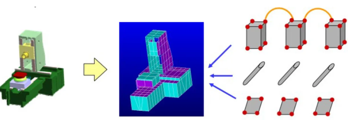
The development of the FEA in continuum mechanics is often based on an energy principle, e.g., the virtual work principle or the minimum total potential energy principle, which provides a general, intuitive and physical basis that has a great appeal to engineers. Mathematically, the finite element method is employed to find approximate solutions of partial differential equations as well as solutions of integral equations or their combinations. The solution approach is usually a numerically based simulation.

In the modeling of the mechanical response of a soft tissue, the finite element method has been employed to solve the established constitutive equation which describes the soft tissue behavior. The comprehensive employment of local infor-mation makes the FEA efficient in describing the shape changes of the soft tissue. On the other hand, with the increase of the computation power of computers, the finite element based modeling becomes an efficient and accurate technique in many applications.

It is important to remember that the order the nodes and elements are num-bered greatly affects the computing time. This is because we get a symmetrical, banded stiffness matrix, which bandwidth is dependent on the difference in the node numbers for each element, and this bandwidth is directly connected width the number of calculations the computer has to do. Computer FEM-programs have internal numbering that optimizes this bandwidth to a minimum by doing some internal renumbering of nodes if they are not optimal.

2.1.2 Finite Element Analysis Theory

(41)

method, and its different steps.

2.1.2.1 Discretization

Discretization is the process of dividing your problem into several small elements, connected with nodes. All elements and nodes must be numbered so that we can set up a matrix of connectivity. The picture to the right shows discretization of a transverse frame into beam elements and discretization of a plane stress problem into quadrilateral elements.

Figure 2.1: Divide the domain into a number of small, simple elements (MIT web)

2.1.2.2 Element Analysis

The element analysis have two key components; Expressing the displacements within the elements, and maintaining equilibrium of the elements. In addition, stress-strain relationships are needed to maintain compatibilty.

(42)

and moments and the corresponding displacements.These results could there-fore be interpreted as being obtained by the governing differential equation and boundary condition of the beam elements.

For e.g. a plane stress problem it is not possible to use an exact solution. The displacements within the elements are expressed in terms of shape functions scaled by the node displacements. Hence, by assuming expressions for the shape functions, the displacements in an arbitrary point within the element is deter-mined by the nodal point displacement.

The section of the structure that the element is representing is kept in place by the stresses along the edges. In the finite element analysis it is convenient to work with nodal point forces. The edge stresses may in the general case be replaced by equivalent nodal point forces by demanding the element to be in an integrated equilibrium using work or energy considerations. This technique is often reffered to as to ”lump” the edge forces to nodal forces.

This requirement result in a relationship between the nodal point displace-ments and forces to be given as:

S = kv + S0 (2.1)

Where:

• S - generalized nodal point forces

• k - element stiffness matrix

(43)

• S0 _{- nodal point forces for external loads}

Computer programs usually have many options for types of elements to choose among.

2.1.2.3 System Analysis

A relationship between the load and the nodal point displacements is established by demanding equilibrium for all nodal points in the structure:

R = Kr + R0 (2.2) K =X j aT_jkjaj (2.3) R0 =X j aT_jS_jo (2.4)

The stiffness matrix is established by directly adding the contributions from the element stiffness matrices. Similarly the load vector R is obtained from the known nodal forces.

(44)

2.1.2.4 Boundary conditions

Boundary conditions are introduced by setting nodal displacements to known values or spring stifnesses are added.

2.1.2.5 Finding global displacements

The global displacements are found by solving the linear set of equations stated above:

r = K−1(R − R0) (2.5)

2.1.2.6 Calculation of stresses

The stresses are determined from the strains by Hooke’s law. Strains are derived from the displacement functions within the element combined with Hooke’s law. They may be expressed generally by:

σ(x, y, z) = D.B(x, y, z).ν (2.6)

Where: • v = ar

• D - Hooke’s law on matrix form • B - Derived from u(x, y, z)

(45)

2.1.3 Finite Element Analysis Stage

A Finite Element analysis consist of three separated stages; Preprocessing, pro-cessing, and postprocessing. A complete finite element analysis is a logical inter-action of these three stages.

2.1.3.1 Preprocessing

As the name indicates, preprocessing is something you do before processing your analysis. The Preprocessing involves the preparations of data, such as nodal coor-dinates, connectivity, boundary conditions and loading and material information.

The preparation of data require considerable effort if all data are to be handled manually. If the model is small, the user can often just write a textfile and feed it into the processor, but as the complexity of the model grows and the number of elememnts increase, writing the data manually can be very time consuming and error-prone. Its therefore neccessary with a computer preprocessor which help with mesh plotting and boundary conditions plotting.

For an example of a simple preprocessor, see the Java-applet on these pages. Her you can change loads, boundary condtitions, mesh and element properties and material. All this is done graphically to minimize the chance of error. The only limitation is that you cannot draw your own geometry, you have to select one of the pregenerated geomtries.

2.1.3.2 Processing

(46)

Figure 2.3: FEA Preprocessing (simplan.de)

2.1.3.3 Postprocessing

The postprocessing stage deals with the representation of results. Typically, the deformed configuration, mode shapes, temperature, and stress distribution are computed and displayed at this stage.

For an example of a simple postprocessor, see the Java applet on these pages. Here you can, after analysis of a model, view the deformed model, and inspect stresses and displacements, both in the controid of elements and the nodal values, and see contour plotting of these data.

(47)

2.1.4 LS-DYNA Solver

LS-Dyna is advanced general purpose multi-physics simulation software developed by Livermore Software Technology Corporation. LS-Dyna is a Non-linear Explicit Transient Dynamic FE code, originated from the 3-D FEA program DYNA-3D developed by Dr.John.O.Hallquist at Lawrence Livermore National Laboratory, California in 1976.

The main application areas of LS-DYNA are crash simulations, metalforming simulations and the simulation of impact problems and other strongly non-linear tasks. LS-DYNA can also be used to successfully solve complex nonlinear static problems in cases where implicit solution methods cannot be applied due to con-vergence problems.

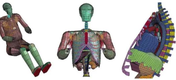
Figure 2.5: Wayne State Human Body Model - II

2.1.5 Multibody Dynamics Simulation

2.1.5.1 Overview

(48)

animation, haptics and virtual reality. A great number and variety of formalisms have been developed for rigid body systems despite the fact that all of them can be derived from a few fundamental principles of mechanics.

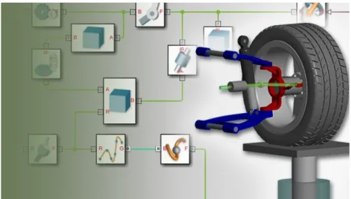
Figure 2.6: Multibody Simulation with Simmechanics (Matworks Inc).

What is commonly known as the Newton-Euler method includes the constraint forces acting on all bodies of the system, which results in redundant equations with more equations than unknowns. In other formulations, such as Lagrange equations, Gibbs-Appell equations [24], and Kanes method [25], the constraint forces are eliminated by use of dAlemberts principle. Efficient simulation algo-rithms were developed based on these formulations for systems with different structures.

2.1.5.2 Matlab SimMechanics Solution

(49)

and aircraft landing gear. The SimMechanics blocks do not directly model math-ematical functions but have a definite physical - mechanical meaning. The block set consists of block libraries for bodies, joints, sensors and actuators, constraints and drivers, and force elements. Besides simple standard blocks there are some blocks with advanced functionality available, which facilitate the modeling of com-plex systems enormously. An example is the Joint Actuator with event handling for locking and unlocking of the joint. Modeling such a component in traditional ways can become quite difficult. The machine is assembled automatically at the beginning of the simulation [? ].

All blocks are configurable by the user via graphical user interfaces as known from Simulink. The option to generate or change models from Matlab programs with certain commands is not implemented yet. It might be added in future re-leases. It is possible to extend the block library with custom blocks, if a problem is not solvable with the provided blocks. These custom blocks can contain other preconfigured blocks or standard Simulink S-functions.

Standard Simulink blocks have distinct input and output ports. The connec-tions between those blocks are called signal lines, and represent inputs to and outputs from the mathematical functions. Due to Newtons third law of action and reaction, this concept is not sensible for mechanical systems. If a body A acts on a body B with a force F, B also acts on A with a force F, so that there is no definite direction of the signal flow. Special connection lines, anchored at both ends to a connector port have been introduced with this toolbox. Unlike signal lines, they cannot be branched, nor can they be connected to standard blocks. To do the latter, SimMechanics provides Sensor and Actuator blocks. They are the interface to standard Simulink models.

(50)

2.2 Literature Review

Figure 2.7: Example of Simmechanics Block Diagram (Matworks Inc).

2.2 Literature Review

2.2.1 Interface Pressure Residual Limb and Prosthesis

2.2.1.1 Finite Element Analysis for Socket Pressure Measurement Socket is an important part of every prosthetic limb as an interface between the residual limb and prosthetic components. Biomechanics of socket-residual limb interface, especially the pressure and force distribution, have effect on patient satisfaction and function.

(51)

this notion because endurance threshold, peak point, and onset of pain are sub-jective and vary from one person to another. Remarkable ethnic differences also exist in terms of genetics, race, muscle intensity, and skin endurance, thereby lowering the credibility of such experiment results. Such comparisons are ongo-ing, and the capability of sensors is further enhanced by technological advances, such as the emergence of chips and ultrasensitive fibers [13]. Aside from sensors, computerized modeling has been also considered since 1996.

Similar to an artificial leg, the residual limb is a complicated system with mechanical and biomechanical behaviors. Parameters, such as force distribution, friction, and tension on residual limb against the socket have been investigated through FEM [99]. Tomographic images have also been used to improve 3D FEM modeling. For instance, liner stiffness and its impact on residual limb-socket fric-tion have been evaluated with the solid model constructed using the automesh function of the CAD system [59]. Understanding these variables helps better in the comprehension of mechanical and biomechanical relationships between the socket and residual limb. However, in several cases of modeling, the displacement during donning the socket is neglected. As such, the automatic contact method was applied to overcome these defects [96] to analyze the magnetic resonance imaging (MRI) and skeletal structure using the Mimics software [56].

(52)

All techniques used for assessing pressure and socket-residual limb tension were aimed at increasing accuracy and producing results approximated to the practical and medical situation. The study on the residual limb-socket interface behavior in a dynamic state has automatically extended the research scope. Some studies have highlighted the mutual effect of the hard and soft tissues of resid-ual limb (e.g., effect of knee movement, changes in the position of residresid-ual limb bones, and their function in generating tension and shear forces). The results of these investigations were expected to contribute to practical improvements in socket construction, mainly for the pain management due to socket misfit. Thus, pain perception was evaluated using technical and computerized systems to re-design and rectify the socket prior to actual construction in accordance with the obtained results [57].

2.2.1.2 Experiments for Socket Pressure Measurement

(53)

The thickness of these sensors and systems, albeit small, affects the results of studies [30, 76]. The accuracy and response of sensors in curved areas, as well as lumps, have also been compared. The only available system that allows clinical use is smart pyramid called Europa. However, it only provides forces applied below the socket, not the forces or pressure applied inside the prosthetic socket or between the residual limb and liner. Yet, the same technology might be improved to be used inside the socket. The current available pressure mapping systems are complicated and expensive and require laboratory settings. These make it impossible to be used in clinical settings. There is the need to develop portable wireless systems that can be easily used in rehabilitation clinics for ob-jective real-time assessment.

2.2.2 Dynamics of Human Gait Analysis

2.2.2.1 Biomechanical Model for Gait Analysis

The characterization of the human body depends on the intended use of the model. The number of segments, the type of joints, the number of muscles, etc., are decisions that researchers have to make according to the purpose of their study.

(54)

provide a realistic representation of the human anatomy.

Figure 2.8: Simple models of human gait. (a) Inverted pendulum model [50]. (b) 2D passive walking [43]. (c) Cornell 3D passive biped with arms [33].

2.2.2.2 Model for amputation patient

(55)

Figure 2.9: Kinematic scheme of human walking with prosthesis with the poly-centric artificial knee joint mechanism [72].

(56)

2.2.3 Ground reaction force and feet pressure

2.2.3.1 Ground reaction force

The ground reaction force (GRF) is the force exerted by the ground on a body in contact with it. For example, a person standing motionless on the ground exerts a contact force on it (equal to the persons weight) and at the same time an equal and opposite ground reaction force is exerted by the ground on the person.

Figure 2.11: Ground reaction force (spartascience.com)

(57)

Figure 2.12: Distribution of the plantar pressures [32].

2.2.3.2 Feet pressure

Feet provide the primary surface of interaction with the environment during lo-comotion. Thus, it is important to diagnose foot problems at an early stage for injury prevention, risk management and general wellbeing. One approach to mea-suring foot health, widely used in various applications, is examining foot plantar pressure characteristics. It is, therefore, important that accurate and reliable foot plantar pressure measurement systems are developed.

(58)

2.3 Conclusion

(59)

Chapter 3 Evaluation interface pressure on

surface of residual limb in

standing posture

The socket of a prosthesis is an important part that serves as the interface be-tween the residual limb and the prosthesis. The soft tissue around a residual limb is not well suited to load bearing and an improper load distribution may cause pain and skin damage. Correct shaping of the socket for appropriate load distribution is a critical process in the design of lower limb prosthesis sockets.

In this chapter, a nonlinear finite element model was created and analyzed to determine the pressure distribution between a residual limb and the prosthesis socket of a transfemoral amputee. Besides that, the better approach for using the shape of socket and residual limb was considered. Three-dimensional models of the residual limb and socket were created using magnetic resonance imaging data; the models were composed of 21 layers, each separated by 10 mm.

(60)

3.1 Introduction

to measure the pressure at eight locations on the surface between socket and residual limb was conducted with the condition correspond with simulation. The value of pressure from experiment and simulation is high coefficient of correlation (>0.817). This analysis allows health care providers and engineers to simulate the fit and comfort of transfemoral prostheses in order to evaluate the fit of socket shape [26].

3.1 Introduction

A lower limb prosthesis is an artificial limb designed to mimic the natural func-tion, structure and aesthetics of the limb being replaces. There are some types of lower limb prosthesis depend levels of lower limb extremity amputations. trans-femoral or above knee prosthetics refers to an artificial limb replacement where the knee joint has been removed and the individual still has part of the femur or thigh bone intact. One of the most important parts of transfemoral prosthesis is a socket, it serves as the interface between the residual limb and the prosthesis. It must not only protect the residual limb, but must also appropriately transmit the forces associated with standing and ambulation. The skin and the soft tissue of the residual limb experiences severe stress and excessive distortion during gait positioning [64]. Especial with transfemoral prosthesis, the residual limb with complex soft tissue and volume change when using sockets. It makes the pros-thesis instability and difficult for patient get acquainted. For evaluate quality in socket design and fit, the pressure distribution at the interface between the resid-ual limb and the prosthetic socket is considered as a main critical. The abnormal effective transfer of force from socket to residual limb is cause of instability of patient gait, pressure ulcers and deep tissue injury.

(61)

3.1 Introduction

focus on the transtibial or below knee prosthesis. The features of residual limb are more convenient to measure or finite element analysis cause the less changing of soft tissue volume, the shape of socket nearly the same with residual limb and the simple displacement in human gait. Damien Lacroix et al. [60] was model the actual donning procedure of socket in five transfemoral amputees and used finite element analysis to observe the stress distribution on the surface of stumps and bone. Linlin Zhang et al. [84] was built a nonlinear finite element model to investigate the interface pressure between the above-knee residual limb and its prosthetic socket. The model of residual limb includes bone and soft tissue and the length of model quite full, along with above hip joint. Portnoy et al [80] was to characterize the mechanical conditions in a muscle flap of trans-tibia patient during static load-bearing. Another study of Portnoy et al. [77] focus on quantifying internal strains in trans-tibia prosthetic user during load-bearing with a variation of residual limb length. It gave more understanding about in-ternal stress and strain of tran-tibia patient and help the prosthetist and patient prevent risk of developing a pressure ulcer and deep tissue injury. Juan Fernando Ramirez and Jaime Andrs Vles [81] were identified the contact boundary condi-tion between bone and soft tissues in a transfemoral amputee affects the stress and strain state of the residual limb.

In this chapter, the authors proposal an overall approach to enhance the eval-uation of the transfemoral prosthesis socket by finite element analysis.

(62)

3.2 Finite element analysis procedures

prosthesis designers in understanding how to better design the socket and trans-femoral prostheses.

After the previous step shown that the approach using different shape of socket get the better results, in this next step, the model of residual limb and socket were created separately. In the model of residual limb includes four parts are bone, muscle, fat and skin. Two types of socket are UCLA and MCCT socket with real size were obtained. The shape of the socket and residual limb are quite different, it makes the computation more complex and spend much more time to complete. Furthermore, the experiment was setting-up to measurement pressure on the interface between socket and residual limb. Eight three dimension sensors were positioned on the surface of the socket for measurement the forces that gen-erate on the skin of the residual limb. The results of simulation and experimental as well as the results of two types of socket were compared and discussed.

3.2 Finite element analysis procedures

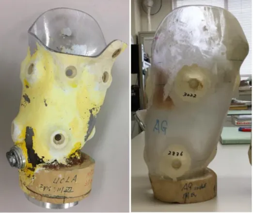
The subject in this study was a male (age 35) with a left-side transfemoral am-putation. He had a height of 169 cm and weighed 63 kg without his prosthesis. The prosthesis incorporated two types of socket are UCLA [17] and MCCT [63] socket, a Nabco prosthesis, and an Ottobock foot.

(63)

UCLA socket while casting. However, the stability in the anterolateral direction was not satisfactory. By applying the force directly to the residual limb while casting that compete with the force generated inside of the socket during gait, it was able to design the IRC socket by which the stability in the anterolateral direction was improved.

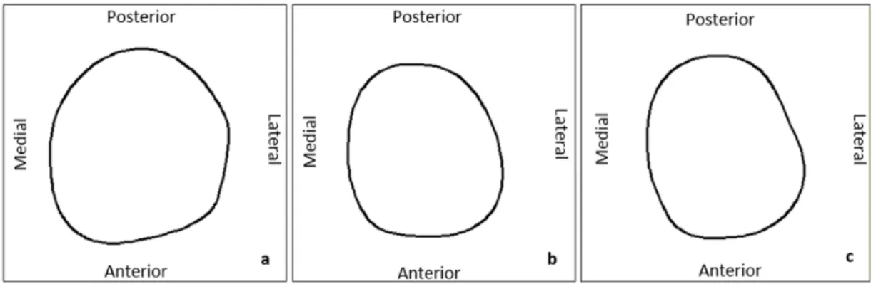
Figure 3.1: Profile at the cross section from distal end of (a) residual limb, (b) UCLA socket, and (c) MCCT socket at 180 mm

3.2.1 Geometry Modeling

(64)

(65)

solid modeling software (PTC Creo Parametric). The model of two type sockets was offset from the skin shape of the residual limb within the socket.

Figure 3.3: 3D model of parts of residual limb. (a. Skin; b. Fat; c. Muscle; d. Bone).

3.2.2 Finite element model

3.2.2.1 Element Types

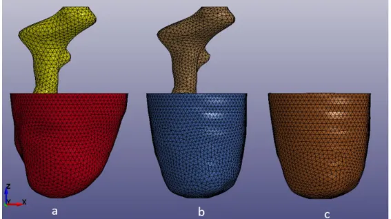
The three dimensional model of all models were meshing with Hypermesh software (Altair Engineering). The socket was meshing as a shell element with thickness about 3 mm. The bone and soft tissue include skin, fat, muscle were meshing with the solid element size of element about 6 mm. The tetrahedral element was used with the type of a solid element. The finite element model of all part was shown on Figure 3.4.

3.2.2.2 Material Model

(66)

Figure 3.4: The FE model of residual limb in case of different shape with MCCT socket (a); same shape with MCCT socket (b) and the socket (c).

with all uniform elastic properties in all directions. Finally, these volumes were assumed to be homogenous with consistent material properties throughout. The femur bone was modeled with a Youngs modulus of 17,700 MPa and a Poissons ratio of 0.3. The prosthesis socket was modeled with a Youngs modulus of 1886 MPa and a Poissons ratio of 0.39 [52].The soft tissue exhibited time-dependent behavior. Fung [22] proposed the quasi-linear viscoelasticity theory that is widely used in mechanics to describe soft tissue behavior. The main assumption of the theory corresponds to the convolution integral representation of the stress as shown in the following expression with respect to an uniaxial loading condition:

σ(t) = Z t 0 G(t)∂σ e_{[λ(τ )]} ∂τ dτ (3.1)

Where σe _{denotes elastic response, G(t) denotes relaxation function, and λ(τ )}

(67)

(3.2) given below:

W = W1+ W2+ W3 (3.2)

The first term W1 aids in modeling the ground substance matrix as a MooneyRivlin material as follows:

W1 = C1(I1− 3) + C2(I2− 3) (3.3)

Where C1 and C2 denote invariants of the right Cauchy deformation tensor.

The second term W2is defined to incorporate the behavior of the crimped collagen

in tension, which works only in the fiber direction as defined in the model given below:

W2 = F (λ) (3.4)

The role of the last term in the strain-energy function is to ensure that the material behaves in an incompressible manner to a significant extent, as given by the following.

W3 =

1

2K[ln(J )]

2 _(3.5)

where J = detF denotes the third invariant of the deformation tensor, which changes based on the volume, and K denotes the bulk modulus. The reduced relaxation function G(t) represented by the Prony series is as follows:

G(t) = 2 X i=1 Siexp( −t Ti ) (3.6)

Here, Si and Ti denote the spectral strength and characteristic time, respectively.

In the study, W1 and W3 were used for skin, fat, and muscle [? ? ]. Table 1 lists

(68)

Table 3.1: Material properties of soft tissues

Name Density C1 C2 S1 S2 T1 T2 K

(kg/m3₎ _(kPa) _(kPa) _(ms) _(ms) _(kPa)

Skin 906 0.186 0.178 0.968 0.864 10.43 84.1 20000

Fat 906 0.19 0.18 1 0.9 10 84 20000

Muscle 1051 0.12 0.25 1.2 0.8 23 63 20000

3.2.2.3 Contact definitions

The first contact definition between the residual limb and the socket was a surface-to-surface contact. A coefficient of friction of 0.5 was assigned as an interaction property for the contact surfaces, as was justified in the previous study [98]. The second contact definition applied a tie contact between bone and muscle. It pro-vides a simple way to bond surfaces together permanently, which prevents slave nodes from separating or sliding relative to the master surface. This contact was suggested from study of Juan Fernando Ramirez and Jaime Andrs Vles [40]. Based on the hypothesis about the connection between skin and fat, fat and mus-cle which there is no movement relation.

3.2.2.4 Loads and boundary condition

(69)

3.3 Interface Pressure Experiment Procedures

3.3.1 Experiment Setup

Figure 3.5: Experiment diagram

(70)

[kP a] = V C

g

4.52_π10−12 (3.7)

Figure 3.6: The position of eight sensors on socket

where g denotes the acceleration due to gravity, 4.5 denotes the radius of the sensor surface, V denotes the voltage generated, and C denotes the calibration coefficient.

3.3.2 Experiment Results

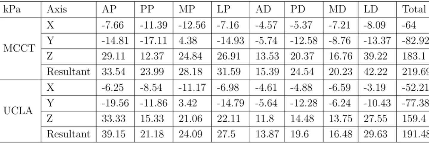
The Table 3.2 and Table 3.3 were shown the value of stress along three axis of sensors in two cases: 50 percent and 100 percent of body weight, which corre-sponding with the stand of patient by one leg and two legs. The results also shown with two types of socket.

(71)

Table 3.2: Stress along the axes of sensor in case of 50% body weight (Unit: kPa)

kPa Axis AP PP MP LP AD PD MD LD Total

MCCT X -7.66 -11.39 -12.56 -7.16 -4.57 -5.37 -7.21 -8.09 -64 Y -14.81 -17.11 4.38 -14.93 -5.74 -12.58 -8.76 -13.37 -82.92 Z 29.11 12.37 24.84 26.91 13.53 20.37 16.76 39.22 183.1 Resultant 33.54 23.99 28.18 31.59 15.39 24.54 20.23 42.22 219.69 UCLA X -6.25 -8.54 -11.17 -6.98 -4.61 -4.88 -6.59 -3.19 -52.21 Y -19.56 -11.86 3.42 -14.79 -5.64 -12.28 -6.24 -10.43 -77.38 Z 33.33 15.33 21.06 22.11 11.8 14.48 13.75 27.55 159.4 Resultant 39.15 21.18 24.09 27.5 13.87 19.6 16.48 29.63 191.48

(stress along x and y axis) in two cases of socket are similar.

In the case of 100% body weight, the maximum normal stress (stress along z axis) is the same with two types of socket. The maximum of normal stress with MCCT socket reached 66.06 kPa at the lateral distal position, with UCLA socket reached 57.28 kPa at the same position in case of MCCT socket, lateral distal. The total of normal stress with MCCT socket is the same with UCLA socket, 298.19 kPa in comparison with 299.23 kPa. The total of resultant stress of MCCT socket is only larger than UCLA socket 1.7%. The direction and magnitude of shear stress (stress along x and y axis) in two cases of socket are nearly the same, except in lateral distal position, the direction of shear stress along x-axis are op-posite.

The load applied to the residual limb in second case increase by double, but the normal stresses are not corresponding rise, total normal stress increases 62.84% in the case of MCCT socket and 88.05% in case of UCLA socket, total resultant stress increase 45.61% in the case of MCCT socket and 64.27% in the case of UCLA socket.

(72)

3.4 Discussion

Table 3.3: Stress along the axis of sensor in case of 100% body weight (Unit: kPa).

kPa Axis AP PP MP LP AD PD MD LD Total

MCCT X -7.07 -12.19 -11.65 -7.07 -4.37 -4.25 -6.49 -2.48 -55.58 Y -15.72 -14.85 4.66 -16.25 -4.49 -11.02 -7.81 -4.53 -70.02 Z 42.17 18.92 39.38 40.89 27.96 32.7 30.11 66.06 298.19 Resultant 45.56 26.96 41.33 44.57 28.65 34.77 31.78 66.26 319.88 UCLA X -4.81 -8.58 -8.98 -7.17 -3.92 -2.74 -6.11 3.6 -38.72 Y -19.59 -6.87 7.01 -16.61 -3.23 -10.97 -3.95 -2.79 -57 Z 47.3 32.41 40.43 37.44 26.56 29.59 28.22 57.27 299.23 Resultant 51.42 34.22 42.01 41.58 27.04 31.68 29.15 57.46 314.55

on eight positions of surface between socket and residual limb is not so different compare with in case of 50 percent body weight. The reason of this is the shape of UCLA more fitting than the shape of MCCT socket. In case of 50 percent body weight, the contact area between socket and residual limb with UCLA socket is more than MCCT socket. This will be clear with the results of simulation.

3.4 Discussion

3.4.1 The comparison of two case residual limb shape

(73)

3.4 Discussion

(74)

3.4 Discussion

pressure at correspond locations doesn’t correlate, the correlation coefficient be-tween the results of experiment and simulation about 0.053.

The comparison of interface pressure between experiment and simulation in the case of the shape of the socket and residual limb are different was shown in Figure 3.7b. The results of simulation distribution from 19.920 kPa at LP location to 34.290 kPa at AD location. The value of experiment always larger than value of simulation from 33.10% at LP location to 73.40% at MD location. However, the results of experiment and simulation have a strong correlation, the correlation coefficient about 0.978. The Figure 3.8 shows the relation between experimental results and two cases of simulation results.

Figure 3.8: The scatter diagram shows the relation between experimental results and two cases of simulation results.

芝浦工業大学学術リポジトリ

Evaluation of Trans-femoral

Prosthesis Function Using Finite

Element Analysis

Acknowledgments

Abstract

Nomenclature

Contents

List of Figures

List of Tables

Chapter 1

Introduction

1.1

Overview

1.1.1

Statement of amputations

1.1.2

Solution for amputation patients

1.2

Transfemoral prosthesis components

1.2.1

The socket

1.2.2

Suspension system

1.2.3

Knee joint

1.2.4

The pylon and ankle

1.2.5

Prosthetic feet

1.3

Common problem

1.3.1

Socket fitting

1.3.2

Dynamics of knee joint

1.3.3

Ground reaction forces and center of preessure

1.4

Objectives

1.5

Contributions

1.6

Structure of this works

Chapter 2

Technical Background and

Literature Review

2.1

Technical Background

2.1.1

Finite Element Analysis

2.1.2

Finite Element Analysis Theory

2.1.3

Finite Element Analysis Stage

2.1.4

LS-DYNA Solver

2.1.5

Multibody Dynamics Simulation

2.2

Literature Review

2.2.1

Interface Pressure Residual Limb and Prosthesis

2.2.2

Dynamics of Human Gait Analysis

2.2.3

Ground reaction force and feet pressure

2.3

Conclusion

Chapter 3

Evaluation interface pressure on

surface of residual limb in

standing posture

3.1

Introduction

3.2

Finite element analysis procedures

3.2.1

Geometry Modeling

3.2.2