Study on stress fields in a V-Shape notched disk under distributed load.
Samadder LITON KU M AR
?, Yoshio ARAI
??, Eiichiro T SU CHIDA
??A new method is developed for determining the stress and displacement
fields around a sharp V-shapenotched disk which is symmetrically loaded on the circumferential edge. Complex eigen function expansion is used to satisfy the stress free condition of the sharp V-shape notch. Boundary condition of the external load applied on the circumferential edge is satisfied with the aid of the Schmidt method. An example of numerical calculation on the stress
field is presented and examined. Approximation expressions based onthe eigen function expansion are proposed and its validity is confirmed. Finally, the numerical results are compared to photoelastic experiment.
Key words:
Eigenvalues, Photoelastic, Stress Singularity, Schmidt method, V-shape notch.
1. Introduction
Sharp corners are often found in welded joints, microelectronic chips, etc. and its structural integrity has recently become increasingly important. Williams
(1)analyzed wedge with variety of edge boundary con- ditions. He noted that a power stress singularity (σ
ij ∝Kr
λ−1) can exist at the apex of the wedge.
He also noticed that an arbitrary loading along the circumferential boundary can be formed by a linear combination of the eigen functions. Many studies have been done on the stress singularity and stress intensity factor of the V-shape notch
(2−8). The sin- gular term describe the stress
field just ahead of theapex of the notch. When the notch opening angle is large the singularity is not strong and the higher or- der terms of the eigen functions are necessary for pre- cise expression of the stress
field around the notch.In this paper, Papkovich-Neuber displacement po- tentails are used to determine the stresses and dis- placement equations. A new analytical method is developed to calculate the stress and displacement around a sharp V-shape notch in homogeneous elas- tic disk which is symmetrically loaded. Numerical calculations are carried out when the external loads are applied to the circumferential edge of the disk.
The external boundary load condition are satisfied with the help of the Schmidt method. Approxima- tion expressions based on the eigen function expan- sion are proposed and its validity is confirmed. Fi- nally, the numerical results are compared to
?Graduate Student of Saitama University
??Departmentof Mechanical Engineering, Saitama Uni- versity
255 Shimo-Okubo, Sakura-Ku, Saitama-Shi, Japan.
photoelastic experiment.
2. Method of Solution
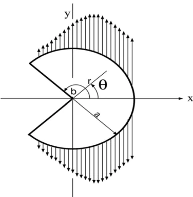
Consider V-shape notched disk subjected to ex- tension in its plane. The opening angle of the notch is 2(
π-b). Let the origin of coordinates be at the center of the circular plate and the relation of the Cartesian and polar system by x = r cos θ, y = r sin θ and the radious of the disk is a. Based on the Papkovich- Neuber potentials formulation, ϕ
0, ϕ
1and the radial and tangential displacement components, u
r, u
θ, are given as follows
(9):
2Gu
r= ∂ϕ
0∂r + r cos θ ∂ϕ
1∂r
−κ cos θϕ
1, 2Gu
θ= 1
r
∂ϕ
0∂θ + cos θ ∂ϕ
1∂θ + κ sin θϕ
1,
⎫⎪
⎪⎪
⎬
⎪⎪
⎪⎭
(1)
where,
∇2ϕ
0=
∇2ϕ
1= 0 and κ is defined as follows:
κ =
(
3
−ν
1 + ν (plane stress), 3
−4ν (plane strain),
where, ν is Possion’s ratio, G is shear modulus. The boundary conditions of this problem are
(σ
θ)
θ=±b= (τ
rθ)
θ=±b= 0, (σ
r)
r=a= p
oσ
r(θ), (τ
rθ)
r=a= p
oτ
rθ(θ).
⎫⎬
⎭
(2)
Among the boundary conditions, the
first bound-ary condition is the stress free boundary condition of
(原稿受付日:平成18年 4月17日)
Figure 1: Circular plate subjected to distributed load on the circumferencial edge
the notch and the second and third boundary con- ditions are external load on the circumferencial edge defined as follows:
σ
r(θ) = 1
2 (1
−cos 2θ) cos πθ 2b , τ
rθ(θ) = 1
2 sin 2θ cos πθ 2b .
⎫⎪
⎬
⎪⎭
(3) Displacement potential function, ϕ
0, ϕ
1, are expressed into harmonic function in polar co-ordinate,
ϕ
0= p
0X∞ n=0
r
λn+1A
ncos(λ
n+ 1)θ, ϕ
1= p
0X∞ n=0
r
λnB
ncos λ
nθ,
⎫⎪
⎪⎪
⎬
⎪⎪
⎪⎭
(4)
where, λ
n, A
n, B
nare the eigenvalues and the un- known constants respectively to be determined from boundary conditions. The equation of the stress and displacement
fields have been developed using Eq.(1)and Eq.(4) .
σ
r= p
0 X∞ n=0λ
nr
λn−1[A
n(λ
n+ 1) cos(λ
n+ 1)θ +B
n{λ
n−κ
2 cos(λ
n+ 1)θ + λ
n−3
2 cos(λ
n−1)θ
}], (5) σ
θ=
−p
0X∞ n=0
λ
nr
λn−1[A
n(λ
n+ 1) cos(λ
n+ 1)θ +B
n{λ
n−κ
2 cos(λ
n+ 1)θ + λ
n+ 1
2 cos(λ
n−1)θ
}], (6)
τ
rθ=
−p
0X∞ n=0
λ
nr
λn−1[A
n(λ
n+ 1) sin(λ
n+ 1)θ +B
n{λ
n−κ
2 sin(λ
n+ 1)θ + λ
n−1
2 sin(λ
n−1)θ
}], (7)
2Gu
r= p
0 X∞ n=0r
λn[A
n(λ
n+ 1) cos(λ
n+ 1)θ +B
nλ
n−κ
2
{cos(λ
n+ 1)θ
+ cos(λ
n−1)θ
}], (8)
2Gu
θ=
−p
0X∞ n=0
r
λn[A
n(λ
n+ 1) sin(λ
n+ 1)θ +B
n{λ
n−κ
2 sin(λ
n+ 1)θ + λ
n+ κ
2 sin(λ
n−1)θ
}]. (9) By using the stress free boundary condition, the characteristic equation can be exprssed into following forms:
λ
2n(λ
n+ 1)(λ
nsin 2b + sin 2λ
nb) = 0. (10) The relationship between unknown constants A
nand B
ncan also be expressed into following forms;
B
n=
−2(λ
n+ 1) cos(λ
n+ 1)bA
n/
{(λ
n−κ) cos(λ
n+ 1)b +(λ
n+ 1) cos(λ
n−1)b
}.
(11) For calculating eigenvalues the characteristic equation is solved by using the Newton-Raphson method.
To satisfy the boundary conditions of the circumfer- encial edge, the Schmidt method is used
(10). The cal- culated stresses can be expressed into complex form as follows:
(σ
r+ iτ
rθ)
r=a= p
0X∞ n=0
A
nW
n(θ), (12) where, W
n(θ) = W
rn+ iW
θn, i =
√−
1, W
rn= λ
n[(λ
n+ 1) cos(λ
n+ 1)θ +R
n{λn2−κcos(λ
n+ 1)θ +
λn2−3cos(λ
n−1)θ
}], W
θn=
−λ
n[(λ
n+ 1) sin(λ
n+ 1)θ
+R
n{λn2−κsin(λ
n+ 1) +
λn2−1sin(λ
n−1)θ
}],
⎫⎪
⎪⎪
⎪⎪
⎪⎬
⎪⎪
⎪⎪
⎪⎪
⎭
R
n=
−2(λ
n+ 1) cos(λ
n+ 1)bA
n/
{(λ
n−κ) cos(λ
n+ 1)b
+(λ
n+ 1) cos(λ
n−1)b
}.
W
n(θ) can be expanded into an orthogonal function
series S
o, S
1, S
2, ...S
n. External load can also be ex-
panded into the orthogonal function series and we
get the following relationship;
(σ
r+ iτ
rθ)
r=a= p
oX∞ m=0
L
mS
m(θ)
= p
oX∞ n=0
A
nW
n(θ), (13) where, S
m(θ) can also be expressed by series of W
l(θ) and the equation can be expressed by following forms;
S
m(θ) =
Xml=0
M
lmM
mmW
l(θ), (14)
L
i=
Rb−b
(σ
r(θ) + iτ
rθ(θ))S
idθ
I
i,
I
i=
Z b−b
S
iS
idθ.
M
lmis the minor of the element d
(l+1)(m+1)in the matrix d
np.
d
np=
Z b−b
W
n, W
pdθ(n, p = 1, 2, 3...m). (15) W
pis defined as complex conjugate of W
p. From Eq.(15) and the boundary condition, Eq.(14), we can get
X∞ n=0
A
nW
n(θ) =
X∞ m=0L
mXm
l=0
α
mlW
l(θ), (16) where, α
ml=
MMlmmm
. We can rewrite the right side of this equation as,
X∞ m=0
L
m Xml=0
α
mlW
l(θ)
=
X∞ m=0X∞ n=m
L
mα
nmW
m(θ). (17) From equation (16) and (17) the unknown constants, A
n, can be expressed into following equation;
A
n=
X∞ m=nL
mα
mn. (18)
Table1: Calculated eigenvalues, λ
nfor k=9 λ
0= 0.5444837367
λ
1= (1.6292573767, 0.2312505471) λ
2= (2.9718437731, 0.3739312054) λ
3= (4.3103772915, 0.4554935790) λ
4= (5.6471117736, 0.513683812) λ
5= (6.9828704415, 0.559108261) λ
6= (8.3180336878, 0.5964194271) λ
7= (9.6528039491, 0.6280993597) λ
8= (10.9872997833, 0.6556354568) λ
9= (12.3215956354, 0.6799917174)
Table2: Calculated A
nfor k=9 A
0= (
−0.43874054,
−3.8344519
×10
−18)
A
1= (
−4.6860928
×10
−2,
−6.30572053
×10
−18) A
2= (
−2.029204
×10
−3,
−4.7431015
×10
−18) A
3= (4.166764
×10
−4,
−7.2929320
×10
−19) A
4= (
−1.7237520
×10
−4, 8.1394037
×10
−19) A
5= (8.502311
×10
−5,
−2.0991458
×10
−19) A
6= (
−5.1531855
×10
−5,
−3.2732869
×10
−19) A
7= (3.1820187
×10
−5,
−5.3546784
×10
−19) A
8= (
−2.2444078
×10
−5,
−4.5320629
×10
−19)
A
9= (1.54729739
×10
−5,
−4.8304523
×10
−19)
3. Numerical AnalysisEigenvalues are calculated when the opening an- gle of the notch 2(π-b)=90
◦. Firstly, characteristic equation (Eq.(10)) is solved by the Newton-Raphson method. Infinite number of complex eigenvalues ex- ist. Calculated eigenvalues are listed in Table1. First eigenvalue is real and the rest of eigenvalues are com- plex. It is certified that the stress free boundary con- ditions (σ
θ=τ
rθ=0 at θ=
±b) are satisfied with the calculated eigenvalues numerically. Using the Schmidt method the distributed load on the circum- ferencial edge (Eq.(3), ”Original” in Fig.2) are ex- panded into the orthogonal function series (Eq.(13),
”Expanded” in Fig.2). The calculation error have the maximum value at θ=0 and the error is 4.8%.
By using the Schmidt method unknown constants, A
n, are calculated and listed in Table1. These con- stants are real. Stress distributions are shown in Fig.3. The large tensile stresses occure at θ=0 for σ
θand θ=
±135
◦for σ
r. Comparing Fig.2(a) (
σpro
= 0 at θ=0) and Fig.3 (
σpro ∼
= 0.6 at θ=0) it is cleared that the bi-axial stress
field is developed due to theconstraint effect of the notch.
To calculate the stresses distribution in the V- shape notched disk under distributed load we pro- pose following relationships:
σ
r= p
on=kX
n=0
A
nW
rnr
λn−1, (19)
σ
θ= p
on=kX
n=0
A
nW
θnr
λn−1, (20)
τ
rθ= p
on=kX
n=0
A
nW
rθnr
λn−1. (21)
W
θn=
−λ
n[(λ
n+ 1) cos(λ
n+ 1)θ +R
n{λ
n−κ
2 cos(λ
n+ 1)θ + λ
n+ 1
2 cos(λ
n−1)θ
}].
(a)
(b)
Figure 2: Comparison between external distributed load and its expanded result
Figure 3: Stress distribution along the circumferential direction
Figure 4: Comparison between exact solution and asymptotic solutions for tangential stress σ
θdistribution along radial direction
(a) Linear plot
(b) log-log plot
Figure 5: Stress distribution along radial direction W
rnand W
rθnare already given in Eq.(13). Fig- ure 4 shows the comparison of full and asymptotic solutions. In the
figure (σ
θp
o)
θ=0is the full solution
(k
→ ∞in Eq.(20)). k=0 is the
first order asymp-totic solution, k=1 is the summation of the
first andsecond order asymptotic solutions. The ranges of ap- plicability of the asymptotic solutions are
ra ≤0.01 for k = 0, and
ar ≤1 for k=1 with the error of less than 0.1%. Figure 5 illustrates that the summa- tion of the
first and second order asymptotic solutiongives reasonable approximation for σ
θ−r relation at θ =0.
Figure 5(a) shows the stress distribution along the radial axis at θ = 0. σ
θis the maximum stress distribution and τ
rθis the minimum stress distribu- tion. Figure 5(b) shows the log-log plot of the stress distribution along the radial axis. Straight line rela- tionships are shown close to the apex of the notch.
4. Comparison with experiment
To compare the calculated result of the difference of principle stresses with experimental result, pho- toelastic experiments have been done. In analytical model the boundary condition on the circumferen- tial edge (Eq.(3)) is the stress distribution of uniax- ial tension, σ
r(θ) =
12(1
−cos 2θ), τ
rθ(θ) =
12sin 2θ, times cos
πθ2b. cos
πθ2bis needed for the notch edge stress free condition. This boundary condition in the analytical model is considered to be similar to the stress
field around V-shape notch in a strip sub-jected to uniaxial tension because the remote stress
fields for the both models are uniaxial tension. Fromthis reason, in this study, the analytical results about V-shape notched disk are compared with the experi- mantal results of the V-shape notched strip. A speci- men shown in Fig.6 which has two V-shape notch(opening angel 2(π-b)=90
◦) in both sides of the strip were ma- chined out from a epoxy plate. Then this strip was annealed to remove the residual stresses of the mate- rial. In annealing process,
firstly 1 hour is needed toarise the room temperature to 120
◦C. Secondly, this temperature was kept for 40 minutes. Thirdly, the temperature is gradually down 10
◦C /hr and if the temperature reached to 80
◦C, the annealing process was stopped. The specimen was set to the photoelas- tic experiment equipment where the tensile load was applied. For photoelasticity the following relation can be used to determine the difference of principle stresses:
σ
1−σ
2= n
αd , (22)
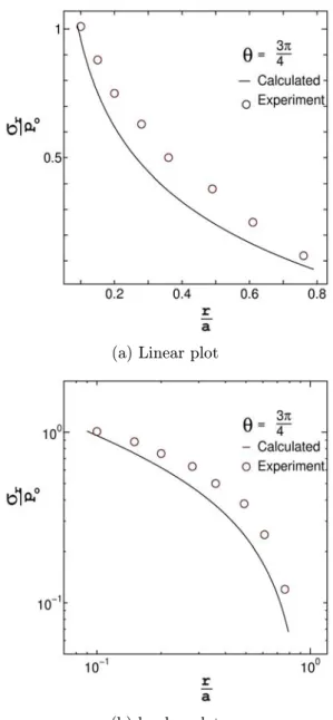
where, n is fringe order, α is the photoelastic con- stant (0.96 mm/kgf for the material used), d is thick- ness of the specimen. Figure 7 shows the fringe pat- tern in the specimen around V-shape notch. Figure 8 gives the comparison between the experimental re- sults and the numerical results for σ
rat θ =
34π (along the notch edge). The distribution character- istics are in good agreement qualitatively.
Figure 6: Specimen configuration (unit: mm)
(a) Bright
field(b) Dark
fieldFigure 7: Photoelastic experiment result. (p
o=7.2 MPa)
The distribution of the difference of principal stresses along the tangential direction are shown in Figure 9.
The qualitative agreement (between the calculated
results and the experimental results ) in tangential
direction of the stresses is also verified. Figure 8 and
9 suggest that the result of the present analysis is
valid to evaluate the stress distribution around the
V-shape notch strip qualitatively.
(a) Linear plot
(b) log-log plot
Figure 8: Comparison between experimental and numerical results along the radial direction
Figure 9: Comparison between experiment and nu- merical result (tangential distribution)
5. Conclusion