Trade Patterns and Brain Drain with Public Human Capital Formation

Trade Patterns

and Brain Drain with

Public Human Capital Formation

Chong Fatt Seng*

Abstract

We examine the relationship between trade patterns and brain drain with publicly pro-vided education service which controls human capital formation. We apply Ricardo-Vin-er model to show that when human capital mobility is allowed in a free trade world, brain drain does not occur necessarily in a country which exports the good using human capital.

key words Human Capital, Brain Drain, Overlapping Generations, Life Time Income,

Trade Pattern

* I gratefully acknowledge valuable comments from Professors Masayuki Okawa, Yutaka Horiba. In particular, I am very grateful to Professor Kenzo Abe (Osaka University) for kindly guidance and heartfelt encouragement. I am solely responsi-ble for any errors.

1） See, for example, a 1984 report (July 20) by the United Nations Conference on Trade and Development (UNCTAD).

It is widely known that skilled workers tend to migrate from developing countries to advanced industrial nations1）_{. Developed countries usually have the comparative advantage in the production of high-tech} good using skilled workers, in the meantime, skilled workers also get higher wage compared to developing countries. This also implies that skilled workers prefer to migrate to developed countries as long as they prefer higher wage. However, this violates the basic propositions in the frame work of Ricardo-Viner (RV) model, i.e., a country with larger supply of skilled workers which are specific to hich-tech sector, has the

comparative advantage in the production of the good, but lower factor price for skilled workers.

This paper incorporates public human capital formation into the basic model of Findlay and Kierzkowski (1983) to provide an explanation of the issue above. They construct a model with two kinds of individual with equal lifetime incomes in terms of present value which is based on the standard Heckscher-Ohlin-Samuelson Model 2）. They show the additional effects of the change in prices compared to the convention-al model. In their model, publicly provided education service does not exit and the education cost is fully fi-nanced by the students 3）.

In this paper, there are three kinds of factors, that is, capital, unskilled workers and skilled workers which are refered as human capital. However, the human capital is assumed to be produced by government through public service in our model. Government can reallocate more human capital into the public sector by extracting human capital 4）from the private sector.

This paper shows that the supply of human capital does not necessarily increase even if government em-ploys more educators for public sector. On the issue between international trade and brain drain , this paper also shows that even if a country exports a good using human capital which is specific factor, the factor price for the human capital in the country can still be higher than that in the foreign. As a result, the human capital flows from the foreign into the country. This result is opposite from the traditional RV model, which does not help to explain the relationship between trade patterns and factor mobility in most cases for many countries.

Miyagiwa (1991) and Wong and Yip (1999), emphasize the role of increasing returns to scale in educa-tion and overlapping-generaeduca-tions model of endogenous growth, respectively. Compared to their studies, this paper presents only a very simple model following the basic assumptions such as constant returns to scale in education and perfect competition in private sectors, but still provide some explanations for the issue of human capital mobility between advanced industrial countries and developing countries. Other than that, this paper also examines whether a government can enhance the competitiveness of high-tech sector by hir-ing more educators.

The model is presented in the next section. The effects of public service are examined in section 3. Our proposition about the trade patterns is obtained in section 4. In section 5, we discuss the issue of brain drain. Some remarks on our conclusion appear in the final section.

2） Mayer (1982), shows factor quality considerations into Heckscher-Ohlin framework and examines the importance of factors skills in determining a country's production pattern and income distribution, while Mayer (1991) shows also the impacts of world price, capital endowment on labor supply, output and national income.

3） Although there is a trend that many universities start charging tuition to the students in many countries, but the role of publicly provided education service is still significant nowadays. In order to make our results more clearly, we focus only on the role of publicly provided education and assume that privately provided education does not exit, which is crucially different from Findlay and Kierzkowski (1983).

The Model

We introduce a country with public human capital formation. There are two private and one public sectors in the country, where one of the private sectors produces high-tech final good using human capital and skilled workers, while the other private sector produces low-tech final good using physical capital and un-skilled workers5）. Unskilled workers is mobile between private sectors while human capital and physical capital are factor specific to high-tech sector and low-tech sector, respectively. Public sector provides edu-cation service to the students for free. We assume that only educators are required for the eduedu-cation service. Therefore, the public sector produces human capital using only educators and students 6）_{. For the time} be-ing, let us show the standard RV model here. The production functions are expressed as7）

where

X

1,

X

2,

L

1,

L

2,

H

pand

K

are high-tech final good produced in hightech sector (i.e., sector 1), low-tech final good produced in low-low-tech sector (i.e., sector 2), unskilled workers employed in high-low-tech sector and low-tech sector, human capital specific to high-tech sector and physical capital specific to low-tech sec-tor, respectively. Let

W

L,

W

Hand

r

denote the factor prices of unskilled workers, human capital and physical capital, respectively. Using the unit cost functions8）, the final goods market equilibrium condi-tions will be given by

where low-tech good serves as the numeraire, and

P

is the relative price of high-tech good in terms of the numeraire. Full employment conditions are expressed as

5） At the present moment, we implicitly assume a small open country model.

6） Educators are also regarded as human capital. On the other hand, students themselves also become the human capital after graduation.

7） Cobb-Douglas functions will make our analysis become simpler. Moreover, we can obtain sharper results easily com-pared to those general functions which will not make significant difference.

8） The unit cost functions are defined as

and

(1)

(2)

(3)

Given

P, K, L, H

p,

α

and

β

, we can solve for

W

L

, W

H

, r, X

1and

X

2from equations (1) to (5).

This is only the familiar basic RV model9）_{which is muchsimpler than what we are going to extend}10）_. At the present model, we only consider a small open country without any international factor mobility. Human capital can be allocated into either private sector (i.e., high-tech sector) or public sector which can be expressed as

H = H

p

+ H

e,

where

H

and

H

edenote the total supply of domestic human capital and the supply of educators, respective-ly.

As in the traditional RV model, we assume the

condi-tions of full employment and perfect competition are always satisfied in the country. However, unskilled workers and human capital are treated as endogenous variables in this paper. We follow the basic concept of Findlay and Kierzkowski (1983)11）_.

_N

_{individuals are born and}

_N

_{individuals die in each period in the} economy, all live for

T

periods. This means that the population will always be

NT

in the steady state12）

We assume education service is publicly provided by government for individuals free of charge in the country, rather than privately provided as assumed in Findlay and Kierzkowski (1983). Either individuals can be “unskilled workers” and immediately start earning

W

Lfor their whole life, or they can become “students,” acquire an “education” that last for a fixed length of time

θ

, and become “skilled workers,”

earning

W

Hfor the fixed length of time (

T

−

θ

). Thus, for each generation,

N = U

l

+ U

e

must be satisfied, where

U

l and

U

e donote the individuals who choose to become unskilled workers and students respectively.

Government employs skilled workers as “educators” from high-tech sector into the public sector. The term of “human capital” in our model includes both skilled workers and educators. We assume that human capital is mobile between high-tech sector and public sector. This means that the government will only pay to the educators with the same going wage for skilled workers. Therefore, education cost is expressed as

W

H

H

e.

The education cost is financed by the income tax13）, then the government budget constraint is expressed as

W

H

H

e

= τ (W

L

L +W

H

H + rK)

,

9） See Jones (1971).

10）L and Hp will be endogenously determined.

11）The pioneering contribution of Kemp and Jones (1962) and elaboration by Frenkel and Razin (1975), Martin (1976) and Martin and Neary (1980) in the literature on variable labor supply are also remarkable.

12）There are T generations and each generation has N individuals. 13）See Abe (1990)

(5)

(6)

where

τ

is the income tax rate14）.

We assume domestic human capital can be produced with Cobb-Douglas production function15）in the public sector which can be expressed as16）

where

γ

can be interpreted as effect of educator-student ratio ( ) on human capital quality, or in other words, on human capital per student ( ) can be acquired by individuals who choose to be edu-cated since it can be expressed as

The government acts like a producer who produces ‘human capital’17）at each period of

t

, using students and human capital itself as inputs18）.

Now, we need to describe how

U

eand

U

lmake their decisions. For simplicity, we also assume that the domestic physical capital stock is owned by all the individuals and there is perfectly equality in distribution of the capital stock19）. Then, in each period of

t

, each individual receives

rk

equally, where

k = K/NT.

The lifetime income after tax for an unskilled worker and skilled worker would therefore result in

respectively, where is fixed interest rate. As Findlay and Kierzkowski (1983) points out, the lifetime in-come after tax for every individuals must be equal in the long run equilibrium, which implies that

14）τcan be solved with this equation, but we do not focus on its effects in this paper. 15）See footnote 7

16）Since θ is assumed to be fixed throughout this paper, differentiation of could be omitted.

17）Compared to Ishikawa (2000) who shows a RV model with an intermediate good. However, in his model, intermediate good is served as input for final good but not for itself.

18）Compared to Becker and Murphy (1992), which show that human capital acquired by a student depends on the human capital of her teachers, and the number of teachers per student. They also note that some good empirical studies like Card and Krueger (1990) and Finn and Achilles (1990) found some evidence to the assumption above.

19）Many studies assume this, for example, see Gupta (1994).

(8)

where 20）

H

and

U

ecan be solved with equations (8) and (9) simultaneously, given

H

e

, W

Land

W

H. Substitut-ing

H

into equation (6) we can solve for

H

p.

U

l can be solved with equation (7). Since there are only 2 generations at each period of

t

, unskilled workers supply is given by

L = U

l

T

.

The model can be solved from equations (1) to (10) to solve for 10 variables, that is,

W

L

,

W

H

,

r

,

X

1

,

X

2

, H

p

, L, U

e

, U

l and

H

, given

P

,

H

e, as well as

α, γ, β, K, N

and

i

which are assumed to be fixed throughout this paper21）.

Preliminaries

Let

N, K

and

i

be fixed throughout this paper. Differentiating equations from (1) to (10), the equations can be reduced as

20）Note that dBH/dUe< 0, where thus we know that Uemust be determined under the arbitrary condition.

21）In particular, Hpand Lcan be solved as functions of (WL,WH, r; ・) while WL, WHand rcan be solved as functions

of (P,Hp, L; ・), where (・) represents other variables treated exogenously. Since WHand rcan also be solved as functions of (P,WL) which is familiar in RVmodel. In the end, the system above can be reduced to 3 equations which

must be solved simultaneously for WL, Hpand L.

(10)

where

denotes a proportionate change, for example, . In particular, notice that

δ

p rep-resents the allocative share of domestic human capital in private sector. In addition, we also have

Equations (12) and (13) are so familiar where the first term in the RHS of equation (12) represents the di-rect effect of human capital on the high-tech good while keeping the factor prices hypothetically constant. We call this effect as the direct effect. The second terms in the

RHS

of equation (12) and

RHS

of equation (13) represent effects on high-tech good and low-tech good, respectively, due to the change in the factor prices which originated from the disturbance in the factor markets. We call this as the indirect effect.

Using Cramel’s rule to solve equation (11), then substitute and into equations (12) and (13), we obtain the direct effects, indirect effects and total effects of

P

,

H

eon

X

1

,

X

2and

X

1

/

X

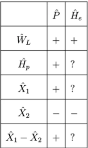
2which are

shown in table 1.

The effects of

H

eon

H

p

,

X

1and

X

1

/

X

2are ambiguous. Since the ambiguous effects mainly originated

from the change in

H

p, in particular, we show that the effects of

H

eon

H

pcan be decomposed into three parts which can be expressed as

(12)

(13)

Table 1: The table shows the effects of P, Heon WL, Hp, X1, X2and X1/X2, respectively. For ex-ample, the effect of Pon WLis shown as‘+’, and so on.‘?’,‘+’and‘−’refer to indefinite effect,

positive effect and negative effect, respectively.

or alternatively,

where

In general, the sign of is not determined, however, we know that the sign is positive (negative) if and only if

where

RHS

is obviously between 0 and 1 since the numerator is smaller than the denominator and both of them are positive as well. In particular, we can see that the condition is satisfied easier with larger

β

and

γ

, but smaller

α

.

The first term in the brace of equation (14) represents the effects on educator-student ratio. Since higher quality of human capital can be acquired as the ratio is higher, we call this as quality effect. The second term in the brace of equation (14) represents the effects on number of individuals who decide to be educat-ed, we call this as quantity effect. The last term represents the input effect which is negative, we call this as crowding out effect. The total effect particularly depends on

δ

p, that is, allocative share of domestic human capital in private sector. In particular, we can conclude as

Lemma 1 In the country with public human capital formation, an increase in

P

always increases the

hu-man capital in private sector. On the other hand, an increase in Heincreases (decreases) human capital in (15)

private sector, if

γ

and

β

are sufficiently large (small) while

α

is sufficiently small (large).

Recall that

γ

represents the effect of educator-student ratio on human capital quality. Larger effect means larger human capital per capita that students can acquire, hence higher productivity and income they can get. This also makes more individuals are willing to choose being educated. The problem is whether the number of students will increase significantly hence overcome the negative crowding out effect. This de-pends on the elasticities of demand for unskilled workers in high-tech sector and low-tech sector, which are donoted by

α

and

β

, respectively. Recall the familiar traditional RV model, if

β

is large and

α

is small, then elasticity of demand for unskilled workers is large in high-tech sector and small in low-tech sec-tor, it follows that higher

W

H

/

W

Lcan be realized hence more individuals are willing to choose being edu-cated.

The indeterminacy of effect of

H

eon

H

palso brings ambiguous effects on

X

1and

X

1

/

X

2. The signs of

and are positive (negative) if and only if

respectively, where

Since

A > 0, B > 0, C > 0, D > 0

,

and

A < B, C < D

, the RHS of equations (17) and (18) are between 0 and 1. It follows that we can conclude the results above as

Lemma 2 In the country with public human capital formation,

(a). an increase in Palways increases X1but decreases X2, hence increases X1

/

X

2, and

(b). an increase in Healways decreases X2.

(c). On the other hand, if

γ

and

β

are sufficiently large (small) while

α

is sufficiently small (large), an increase in Heincreases (decreases) X1

/

X

2as well as X1,

Lemma 2(a) says that

X

1

/

X

2is an increasing function of

P

while lemma 2(c) says that relative supply curve does not necessarily shift to the right due to an increase in

H

e.

(17)

Trade patterns

To see how the relative price of final goods change, the demand side of the final goods has to be stated ex-plicitly. We can express the relative demand which is denoted by

D

as a function of

P

on the demand side, if we assume homothetic preferences 22）. Then the domestic market equilibrium is expressed as

X = D(P),

where

X

≡

X

1

/

X

2. Differentiating the equation above and using the results in table 1, we obtain

where

σ

D≡ −

D’(P)P/D(P)

is the price elasticity of demand.

In the lemma 1 and 2, we have examined the effect of

P

on

X

which is positive, whereas the effect of

H

eon

X

is ambiguous, hence the total effect is ambiguous as well. Let us define that

Definition 1

A country with more (less) human capital employed in private sector is called human capital abundant (scarce) country.

Hence we can establish the following proposition.

Proposition 1

Suppose that there are two countries with public human capital formation where preferences, technology, capital endowment and population are identical. If the effect of educator-student ratio on human capital quality and income share of unskilled workers in low-tech sector are sufficiently large (small), then the country that allocates more domestic human capital into the public sector tends to be human capital abun-dant (scarce) country, hence exports (imports) high-tech final good and imports (exports) low-tech final good.

Again, the argument in the proposition 1 can easily be predicted from the lemma 1 and 2. If an increase in

H

edecreases the human capital supply in private sector instead, then the government will fail to enhance the competitiveness of high-tech sector.

Notice also that since an increase in

H

edecreases

H

pbut increases

H

when

γ

is small23）, if ‘human capital abundant country’ is defined as a country with larger

H

instead of

H

p, then we can conclude as ‘hu-man capital abundant country imports high-tech final good and exports low-tech final good’, which is a paradox24）.

22）Although there are two kinds of individual in this model, identical preferences assumption is unnecessary as long as their lifetime income are all the same as well as their fixed rate of time preferences which are equal to the market rate of interest.

23）See equations (6) and (15.)

24）See Leontief (1956) and Ishizawa (1988), where Ishizawa (1988) shows the Leontief paradox through the public sectors

Foreign Human Capital Mobility

We examine the effect of

H

eon factor mobility among countries in this section, let us focus only on the hu-man capital mobility rather than capital mobility, the effect of

H

eon can be obtained as

From the table 1, we know that

From equation (20) and (21) it is easy to show that

Equation (21) says an increase in

H

ealways decreases

W

H. From equation (9) we can also easily see that

W

His an decreasing function of

H

instead of

H

pwhich is different from the traditional RV model.

Recall the lemma 1 and consider the case of a country where the effect of educator-student ratio on hu-man capital quality and income share of unskilled workers in low-tech sector are sufficiently small, then we have

Equation (23) says that when the country allocates less domestic human capital into the public sector, the human capital employed in private sector increases. In the meantime, equation (22) shows the factor price for human capital in the country rises, which is opposite compared to the traditional effect. Suppose that equation (23) is satisfied. Consider the case in which there are only country

A

and country

B

exit in the world. If country

A

allocates less domestic human capital into the public sector, then country

A

has the comparative advantage in the production of high-tech good but higher wage for skilled workers compared to country

B

, which is totally opposite compared to that in the traditional RV model.

Suppose country

A

is the advanced industrial country while country

B

is the developing country in this case, human capital moves from developing country to advanced industrial country. Recall the words of World Development Report: “Can something be done to stop the exodus of trained workers from poorer countries?” (World Bank, 1995, p. 64)25）.Government can reduce its public service by decreasing the

num-(21)

(22)

(23)

which depends on assumptions of the factor intensities and the size of the economy. Furthermore, the definition of ‘abundant’ may have played a great role to the paradox.

25）See Stark-Helmenstein-Prskawetz 1998.

ber of educator but still can enhance its high-tech sector and improve the brain drain problem. Hence we can conclude as

Proposition 2

Suppose that there are two countries with public human capital formation where preferences, technology, capital endowment and population are identical. If the effect of educator-student ratio on human capital quality and income share of unskilled workers in low-tech sector are sufficiently small, then the country that allocates less educators into the public sector tends to export high-tech final good and have higher fac-tor price for human capital.

Proposition 2 implies that if human capital mobility is allowed between the two countries in a free trade world, human capital moves from the country which exports high-tech final good into the country which imports it. This is the crucial result in the present paper. A government can reduce its educators but still can enhance the high-tech sector. More surprisingly, despite the country becomes human capital abundant country and exports high-tech final good, the wage for human capital rises and creats an incentive for for-eign human capital inflow. As a result, there is an additional positive effect on the output of high-tech final good, instead of crowding out effect brought by brain drain, as long as foreign human capital inflow is al-lowed. Notice that the total human capital supply decreases as a whole, which has caused the rise in factor price for human capital.

Concluding Remarks

In this paper, we have examined the relationships between trade patterns and human capital mobility. We have found that the RV model still can be applied to explain why skilled workers tend to move from devel-oping countries to developed countries. One of the most important characters is that we use only very sim-ple model to capture the human capital formation and derive some different results compared to many stud-ies.

Our results can best be concluded in proposition 2. Some other policy implications can also be discussed. For example, consider the case of foreign human capital inflow. If the effect of educator-student ratio on human capital quality and income share of unskilled workers in low-tech sector are sufficiently large (small), a government should hire foreign human capital to work as educators in education sector (skilled workers in private high-tech sector) to enhance the high-tech sector in a more effective way.

Appendix

A.1

Calculation

Differentiating equations from (1) to (10), we have26）

Since

N

and

K

are assumed to be fixed throughout this paper, hold. Equations (A.1) to (A.5) are the familiar basic equations of the RV model. Considering equations (A.1) and (A.2) can also be rewritten as

we can solve easily given and as

26）Notice that i is fixed.

which is familiar. Substitute equations (A.11) and (A.12) into equations (A.4) and (A.5), we obtain equa-tions (12) and (13).

Using equations (A.6) and (A.8) to solve for , we obtain

Substitute equation (A.8) into equation (A.9) to eliminate and rewrite it by using equation (A.11), we have

Substitute equation (A.7) into equation (A.10) to eliminate

U

l, we obtain

We can also substitute equation (A.15) into equations (A.14) and (A.16) to eliminate , but since we are more interested in the effects on

U

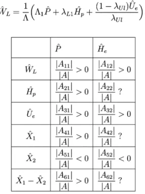
einstead, we substitute equation (A.16) into equation (A.13) to elim-inate , hence we have

Table 2: The table shows the effects of P and Heon WL, HP, Ue, X1, X2and X1/X2,

respective-ly. For example, the effect of Pon WLis shown as |A11|/|A| > 0, and so on. ‘?’ refers to indefinite

From equations (A.14), (A.15) and (A.17), we obtain equation (11) as shown in context.

Using Cramel's rule to solve equation (11), then substitute and into equations (12) and (13), we obtain the results shown in table 2, where

A.2

Decomposition of effects on

H

p

Let us explain why an increase in

H

edoes not necessarily increase

H

p. Rewritting equation (A.14), we ob-tain equation (14) as shown in context.

equations (A.8), (A.9) and (A.11), the quality effect can be expressed as

Since as shown in table 2, the quality effect of

H

eis positive. On the other hand, the quantity effect of

H

eis also positive which can be predicted from as shown in table 2. Thus the sum of the quality effect and quantity effect of

H

eis positive which can be ex-pressed as

Unfortunately, not only the crowding out effect is negative but also the total effect of

H

eon

H

pends up an ambiguous effect which can be predicted from as shown in table 2. The sign is positive (negative) if and only if

where RHS is obviously between 0 and 1 since the numerator is smaller than the denominator and both of them are positive as well. In particular, we can see that the condition is satisfied easier with larger

β

and

γ

, and smaller

α

, hence we have lemma 1. A.3

Domestic market equilibrium

In this subsection, we will show how we obtain the equation (19). Since we know

X

is a function of

P

1and

H

e, while

D

is a function of

P

1, and the domestic market equilibrium which can be expressed as

X(P

1

,H

e

) = D(P

1

).

(A.21)

P

1is determined in equation (A.21) as a function of

H

e, which can be expressed as

Equation (A.21) becomes an identity if we substitute equation (A.22) into equation (A.21), which can be expressed as

Differentiating equation (A.23), we obtain

which can be rewritten as equation (19).

Notice also that the first term and the second term in the bracket of RHS are positive, hence we know that the sign of is negative if

∂X/∂H

e is positive. However, the sign of

∂X/∂H

eis am-biguous in this model.

References

[1] Abe, Kenzo, 1990. “A Public Input as a Determinant of Trade.” Canadian Journal of Economics 23(2), 400-407.

[2] Becker, Gary S.; Kevin M. Murphy, 1993. “The Division of Labor, Coordination Costs, and Knowl-edge.” Becker, Gary S. Human capital: a theoretical and empirical analysis, with special reference to

education.3rd ed. Chicago; London: The University of Chicago Press, Chapter XI, 299-322.

[3] Bhagwati, Jagdish N.; T.N. Srinivasan, 1983. Lectures on international trade. Cambridge, Mass.: MIT Press.

[4] Card, David; Alan B. Krueger, 1990. “Does School Quality Matter? Returns to Education and the Characteristic of Public School in the United States.” NBER Working Paper May.

[5] Dixit, Avinash; Victor Norman, 1980. a dual, general equilibrium approach. Digswell Place, Wel-wyn [England] : James Nisbet. - [Cambridge,Cambridgeshire] : Cambridge University Press.

[6] Finn, Jerem D.; Charles M. Achilles, 1990. “Answer and Question About Class Size: A Statewide Experiment.” American Education Research Journal 27, 557-77.

[7] Findlay, Ronald; Henryk Kierzkowski, 1983. “International Trade and Human Capital: A Simple General Equilibrium Model.” Journal of Political Economy 91, 957-978.

[8] Frenkel, Jacob A.; Assaf Razin, 1975. “Variable Factor Supplies and the Production Possibility Fron-tier.” Southern-Economic-Journal 41(3),410-19.

[9] Gupta, Manash Ranjan, 1994. “Foreign capital, income inequality and welfare in a Harris-Todal mod-el.” Journal of Development Economics 45, 407-414.

[10] Ishikawa, J., 2000. “The Ricardo-Viner Trade Model With An Intermediate Good.” Hitotsubashi

Journal of Economics 41, 65-75.

[11] Ishizawa, Suezo, 1988. “Increasing Returns, Public Inputs, and International Trade.” American

Eco-nomic Review 78(4), 794-95.

[12] Jones, Ronald W., 1971. “A Three-Factor Model in Theory, Trade, and History.” In Trade, Balance

of Payments and Growth: Papers in International Economics in Honor of Charles P. Kindleberger,

edited by Jagdish N. Bhagwati et al. Amsterdam: North-Holland.

[13] Kemp, M.C. and R.W. Jones, 1962. “Variable labor supply and the theory of international trade.”

Journal of Political Economy 70, 30-36.

[14] Leontief, Wassily W., 1986. “Factor Proportions and the Structure of American Trade: Further The-oretical and Empirical Analysis.” Input-output economics. Second edition, New York and Oxford: Ox-ford University Press, 94-128. Previously published: [1956].

[15] Martin, John P., 1976. “Variable Factor Supplies and the Heckscher-Ohlin-Samuelson Model.”

[16] Martin, John P.; J. Peter Neary, 1980. “Variable Labour Supply and the Pure Theory of International Trade: An Empirical Note.” Journal of International Economics 10(4), 549-59.

[17] Mayer, Wolfgang, 1982. “Factor Quality, Factor Prices and Production Patterns.” Journal of

Inter-national Economics 12(1/2), 25-40.

[18] Mayer,Wolfgang, 1991. “Endogenous labor supply in international trade theory.” Journal of

Inter-national Economics 30, 105-120.32

[19] Miyagiwa, Kaz, 1991. “Scale Economies in Education and the Brain Drain problem.” International

Economic Review 32, 743-759.

[20] Stark, O., Helmenstein, C., Prskawetz, A., 1998 “Human capital depletion, human capital formation, and migration: a blessing or a “curse” ?” Economics Letters 60, 363-367.

[21] Wong, Kar-yiu; Chong Kee Yip, 1999. “Education, economic growth, and brain drain.” Journal of