Trade Patterns and Human Capital under Publicly Provided Education and Privately Provided Education

Intoduction

The topic about relation between human capital and trade patterns has been explored by many au-thors. Human capital can be produced through various channels. Education is one of the chan-nels to produce human capital. On the other hand, education can be provided by public sector or pri-vate sector. In fact, there are some countries where education is mainly provided by govern-ment whereas some countries are the opposite.

If human capital is provided by public sector or government, it is interesting to refer some studies in the literature of international trade where pub-lic service or pubpub-lic good is incorporated. Abe (1990) examines how the difference in the level of public input supplied by the government af-fects the trade patterns between the countries. Some other studies are also remarkable such as Manning McMillan (1979), Tawada and Abe (1984), Okamoto (1985), and Ishizawa (1988) al-so examine trade patterns in the economy with the public intermediate good. The important role of

under Publicly Provided Education and

Privately Provided Education

CHONG, Fatt Seng

Abstract

We examine the trade patterns using traditional Ricardo-Viner model, but also consid-er one of the sectoral-specific factor as human capital which will be produced undconsid-er edu-cation. The education service in a country may be provided by government or private sector. We will show that a country with a publicly provided education will export the good which is produced by using the human capital.

要 約 近年、国立大学の独立法人化が進み、従来の国公立大学も私立大学としての特徴が目立 つようになってきた。こうした状況の中で、国際競争力が受ける影響について、理論的な 枠組で分析してみる。特に、貿易パターンへの影響を調べるために、われわれは、人的資 本の概念が導入された伝統的な特殊要素モデルを用いて、極端な二つのケースを検討して みる。つまり、国立大学しか存在しない国と私立大学しか存在しない国における、最終財 の国内相対価格を調べ、最後に貿易パターンを導出する。結果的に、国立大学だけ存在す る国が、人的資本を使って生産される最終財を、私立大学だけ存在する国に輸出すること が示される。 Key words

government which is to provide public input to private sector is emphasized in those studies. There are also some authors consider the public input as education such as Wong and Yip (1999) study the effects on growth, welfare, and income distribution.

However, in the literature of international trade, the comparations between publicly provid-ed service and privately providprovid-ed service, espe-cially where human capital is dealt with, have not been explored sufficiently. The issue of trade pat-terns between publicly provided education econo-my and privately provided education econoecono-my will be examined in this paper.

On the other hand, Findlay and Kierzkowski (1983) construct a model with two kinds of individ-ual with eqindivid-ual lifetime income in terms of present value which is based on the standard Heckscher-Ohlin-Samuelson (HOS) model.１_{In this paper,} we follow the basic idea of Findlay-Kierzkowski (1983) and apply the standard Ricardo-Viner (RV) model instead of HOS model.

The purpose of this paper is to study the trade equilibrium between the public education country and the private education country. We will show that a country with publicly provided education will export final good which is produced by using human capital and import the other final good which is produced by not using human capital, while a country with privately provided education does the opposite. In order to make our compara-tion more tractable, we will simplify all the pro-duction function not only in standard form but al-so in more numerically. Since the basic model we apply here is RV model, analogous production functions are also allowed in this paper.２

In the next section we will simply show the standard RV model, and then the formation of hu-man capital under publicly provided education and privately provided education. The main re-sults are shown in section 3 and the comparations are presented in section 4. Concluding remarks are given in the final section.

The Model

（1）

The Standard Ricardo-Viner model

We consider a three-sector (2 final good sectors and 1 education sector), two-primary-factor (un-skilled labor and capital)framework. Final good sectors are private sectors while education sector may be public sector or private sector. Education sector produces human capital which will be used together with unskilled labor as inputs in one of the final good sectors, say, sector 1, to produce the final goods, say, good 1. Good 2 is produced in sector 2 using the primary-factor, that is, un-skilled labor and capital. On the other hand, hu-man capital is produced using unskilled labor and the human capital itself in the education sector. Unskilled labor is mobile among the private sec-tors and capital is immobile among secsec-tors, whereas human capital is mobile between only sector 1 and education sector.

First, we will show the basic RV model. As-sume that the production functions of the final goods are expressed as

,

X1= L H1 (1)

,

X2= L K2 (2)

where X1, X2, L1, L2, K and H denote good 1, good

2, unskilled labor employed in sector 1 and sector 2, capital and human capital, respectively.

Full employment conditions of the primary-fac-tor are expressed as

,

L1+L2=L (3)

,

K=K (4) where K is the fixed endowment of capital while

L is the supply of total unskilled labor and is en-dogenously determined which is different from the standard RV model.

The basic RV model differs also from our mod-el in the full employment condition of human capital. Assume also that the production function of the education sector is expressed as

,

H H UE E ∼

, H H HE ∼ = - (6) where H ∼

is the gross output of human capital and HEis the input of human capital itself, or we can

refer it as “educator” in the education sector.３_U

E

represents those who have chosen not to be un-skilled labor but to be students. H denotes the net output of the human capital. In other words, H

∼

is the total supply of human capital which can be employed in education sector as educator (HE) or

in the sector 1 to produce good 1. For simplicity, we also assume that the domestic capital stock is owned by all individuals and there is perfectly equality in distribution of the capital stock.４ Then, in each period, each individual receives rK/2N equally where r is the factor price of the capital and 2N is amount of population.

At the present moment, suppose H is assumed to be perfect inelastic, then we can solve the basic system by using the unit cost functions. Let WH

and WLdenote the factor prices of human capital

and unskilled labor, respectively.５_{The final goods} market equilibrium conditions will be given by

, W W P 2 H L= (7) , rW 2 L=1 (8)

where good 2 serves as the numeraire, and P is the relative price of good 1 in terms of the nu-meraire. Full employment conditions are ex-pressed as , X W_W X _Wr L L H L 1 + 2 = ₍₉₎ , X _WW H H L 1 = (10) . X W_rL K 2 = (11)

Given P, K, L, H, α and β, we can solve for WL,

WH, r, X1and X2from equations (7) to (11). This

is only the familiar basic RV model which is much simpler than what we are going to extend.

Now, we have to introduce the basic idea of Findlay and Kierzkowski (1983) to complete our model. In the economy, we have 2 generations at each period. At each period, N individuals are born but also N individuals die, it ends up a

sta-tionary population at each period. For simplicity, we assume that each individual lives for only 2 periods. Each individual can choose to be educat-ed at period 1 then earn his or her income as hu-man capital at period 2, or choose to start working as unskilled labor to earn his or her income at pe-riod 1 and pepe-riod 2. Either way, their lifetime in-come must be the same due to the arbitrary condi-tions. Let UEand UL denote the individuals who

choose to be educated and to be unskilled labor, respectively.

The population at each period is expressed as ,

N U U

2 =2_ E+ Li (12)

it follows that the total supply of unskilled labor is expressed as

.

L=2UL (13)

The next step is to clarify the differences be-tween the publicly provided education and the privately provided education.

（2）

Publicly provided education

In this subsection, we assume that the education is provided by the government with free of charge. The government imposes income tax to finance the provision of education. The opportunity cost, which is the income of unskilled labor earned at period 1 and period 2, in terms of present value,６ is expressed as , W W 1- L+₁ L + x _t _ id n

where τ and ρ are, income tax rate and fixed in-terest rate, respectively. Since the education ser-vice is free of charge, the total cost of education is only the opportunity cost, which is the income of unskilled labor earned at period 1 and period 2. The gross benefit of education to an individual, in terms of present value, is expressed as

. U W H U 1 ₁1 E H E E : : -x _+t _ i Note that W HH ∼

whole supply of human capital at period 2 with-out tax being imposed, that is, when τ is zero.７

In the equilibrium, UEmust be determined with

equalizing the opportunity cost and the gross ben-efit of human capital in terms of present value, thus we must have

. W W U H U 2 H L E E E = +t _ i (14)

The government ’s budget constraint will be given by

,

W HH E=x8WH_H+HEi+W LL +rKB (15)

where the LHS is the tuition received by all edu-cators while the RHS represents the tax revenue collected by imposing the same income tax rate to all individuals.

Assume that the government chooses HEto

maximize H , hence the maximization problem is .

max H

HE

Considering the equations (5) and (6), the solu-tion for the problem is

. U H 4 1 E E ₌ (16) Before we see the equilibrium in the case of publicly provided education, we depict the case of privately provided education in the next subsec-tion.

（3）

Privately provided education

In this subsection we assume that there is no edu-cation is provided by government which is free of charge, so each individual has to “buy ”the educa-tion service. We also assume that each educator gets exactly the factor price of human capital as his or her wage. It follows that tuition has to be paid by an individual is WEHE/UE. The

opportuni-ty cost will be the income of unskilled labor earned at period 1 and period 2. Hence the total cost of education will be given by

. U W H _W W 1 E E E L L + + +t

The gross benefit of education to an individual is expressed as . U W H U 1 1 E H E E : +t

In the equilibrium, the gross benefit must be equal to the total cost of education, thus we must have . WW _U H U H 2 1 H L E E E E = + - + t t _ _ i i (17) As long as the private education sector is per-fect competitive, we must have

, W H H U W H E E E H : 2 ₂ = (18)

which is the familiar first order condition, only is WH in the LHS represents the price of the human

capital which can be “purchased ”by sector 1, whereas the other one in the RHS represents the factor price of the educator. Hence we obtain the exactly same condition in the case of publicly provided education, which is expressed in the equation (16).

Public Provision VS Private

Provision

In this section, we are going to compare the equi-librium between the case of publicly provided ed-ucation and the case of privately provided educa-tion. To see the comparation more clearly and without getting confused, we distinguish the nota-tion of endogenous variables between the two cases. For example, WL

g

will represent the factor price of unskilled labor in the case of publicly provided education whereas WL

p _{will represent}

that in the case of privately provided education. After all, we can use 12 equations to solve for the economy with publicly provided education, that is, from equations (5) to (13) and (14) to (16) to solve simultaneously for 12 variables which are

WL g_{, W} H g_{, r}g_{, X}g 1 , X g 2, L g_{, H}g_{, H} E g_{, H}g ∼ , UE g_{, U} L g_and

equa-tions to solve for the economy with privately pro-vided education, that is, from equations (5) to (13), (16) and (17) to solve for 11 variables which are WL p , WH p , rp_{, X}p 1 , X p 2, L p , Hp , HE p , Hp ∼ , UE p , and UL p_.

Let us solve for WL, WH, r, X1and X2in concrete

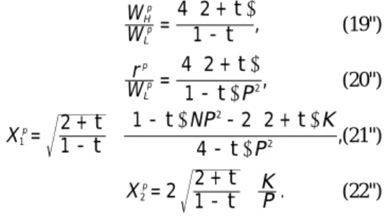
form given P, K, L and H . From equations (7) to (11), we have the conventional RV model solu-tions which are expressed as

, W W HP K LP L H 2 2 = + (19) , Wr HP K L L= 2+ (20) , X HP K LP 1 2 2 = + (21) . X HP K L 2= 2₊ (22)

The four equations above are common to both the cases of publicly provided education and private-ly provided education. The next thing we have to do is to solve H and L in concrete form.

（1）

Publicly provided education

equilibri-um

From here we start using the distinguished nota-tion to avoid confusion. The endogenously deter-mined variables are in the form with superscript of “g” as referred previously. Rewrite the equa-tion (16), we have . U H 4 1 E g E g = (16')

From equations (16'), (5) and (6), we obtain , Hg ₄1 U E g : = (23) . Hg H E g = (24)

Substitute equations (5), (16') and (19) into equation (14) and rearrange it, we have

. L P HP K 2 2 g 2 2 : = _ +ti + (25)

Substitute equations (12), (13) and (23) into equa-tion (25), we obtain , U P 6 NP K 4 ₂ E g 2 2 = +t - +t _ i8 _ iB (26)

where _2_+tiK NP/ 2<1_{is assumed.}８_Substitute equation (26) into equations (23) and (24), we have, . H H P 6 NP K 4 ₂ g E g 2 2 = = +t - +t _ i8 _ iB (27)

Substitute equation (27) into equation (25), we obtain . L P NP K 6 2 2 4 g 2 2 = + + + t t _ _ _ i i i (28) Now we can solve the equations from (19) to (22) in concrete form. Substituting equation (27) and (28) into them, we obtain

, W W 2 2 L g H g = _ +ti (19') , W r P 2 2 L g g 2 = _ +ti (20') , X P NP K 6 2 2 2 g 1 2 2 : = + + - + t t t _ _ ` _ i i i j (21') . Xg 2 2_P K 2 : = _ +ti (22')

In particular, we can also solve for WL g , WH g , rg and Xg 1, X g

2. Rearrange equation (19') and

substi-tute it into equation (7), and then substisubsti-tute WL g in-to equation (20'), we have , W P 2 2 2 L g₌ +t _ i (29) , WH 2 2₂ P g₌ _ +ti: ₍₃₀₎ . rg₌ 2 2__2P+ti (31) On the other hand, from equations (21') and (22'), we obtain . X X KP NP K 6 2 g g 2 1 2 = + - + t t _ _ i i (32) It is interesting to see that WL

g_{/P and W} H

g_{/P are}

alway constant as well as WH g /WL g . The magnifica-tion effect of P on WH g_/W L

g_{vanishes in our model}

（2）

Privately provided education

equilibri-um

In this subsection we will do almost the same sub-stitutions as done in the previous subsection, only we use equation (17) instead of equation (14). Moreover, we use the superscript notations with “p” instead of “g” to distinguish from the case of publicly provided education.

Rewrite equation (16), we have . U H 4 1 E p E p = (16'')

From equations (16''), (5) and (6), we obtain , Hp ₄1 U E p : = (33) . Hp H E p = (34)

Substitute equations (5), (16'') and (19) into equation (17) and rearrange it, we have

. L P HP K 1 4 2 p 2 2 : = -+ ₊ t t _ i (35) Substitute equations (12), (13) and (33) into equa-tion (35), we obtain , U P N P K 4 2 1 2 2 E p 2 2 = -- - + t t t _ _ _ i i i 8 B (36) where 2 2_ _+tiK/_1_-tiNP2<1_{is assumed.}９ Substitute equation (36) into equations (33) and (34), we have . H H P N P K 2 4 1 2 2 p E p 2 2 = = -- - + t t t _ _ _ i i i (37) Substitute equation (37) into equation (35), we obtain . L P NP K 4 2 2 4 p 2 2 = -+ + t t _ _ _ i i i (38) Now we can solve the equations from (19) to (22) in concrete form for the case of privately provided education. Substituting equation (37) and (38) into them, we obtain

, W W 1 4 2 L p H p = _ _-+_tti (19'') , Wr _{1 P} 4 2 L p p 2 = -+ t t _ _ i i (20'') , X P NP K 1 2 4 1 2 2 p 1 2 2 : = _-+ -- - + t t t t t _ _ _ i i i (21'') . Xp 2 ₁2 K_P 2= _- : + t t (22'') As what have been done in the previous sub-section, we can also solve for WL

p_{, W} H

p_{, r}p_{, X}P 1 /

XP

2 . Rearrange equation (19 and substitute it into

equation (7), and then substitute WL p into equation (20'), we have , WL ₂1 P₄ p_{= :} + -t t (39) , W P 1 2 H p_{= :} -+ t t (40) . rp_{= 1}2 : _P1 -+ t t (41) On the other hand, from equations (21'') and (22''), we obtain . X X KP NP K 2 4 1 2 2 p p 2 1 2 = -- - + t t t _ _ _ i i i (42)

Comparations

In this section, let us make some comparations between the case of publicly provided education and the case of privately provided education which can be shown in table 1.

Factor Supplies Factor Prices Output > UE U g E p _{W /W <W /W} H g L g H p L p _Xg _{? X}p 1 1 > HE H g E p _rg_{/W <r /W} L g p L p _Xg_<Xp 2 2 > Hg Hp _{W <W} H g H p _Xg_/Xg_>Xp_/Xp 1 2 1 2 < Lg Lp _rg_<rp > WL W g L p

Table 1: The difference between Xg 1and X

p

1depends on

the interest rate (or time preference rate), as well as the population, capital endowment and relative price of final goods. Xg

1 is probably larger than X p

1 if K/NP is not too

small as well as ρ.

It is interesting to see that, although WH/W

g L g is smaller than WH/W p L p

will-ing to become UEin the case of publicly provided

education than in the case of privately provided education. This can be explained as follows. In the case of public provision, although the gross benefit of becoming a member of human capital is smaller than in the case of private provision, the “total cost” of education is much smaller in the case of public provision than in the case of private provision. This is mainly because the edu-cation service is free of charge under public pro-vision. As a result, it makes the publicly provided education more attractive compared to the pri-vately provided education and more individuals are willing to become human capital. Since the supply of human capital is larger in the public provision economy, factor prices of specific fac-tors are smaller whereas factor price of mobile factor is larger compared to those in the private provision economy.

We should notice that not only factor prices of specific factors are smaller in the publicly provi-sion economy, but also income tax are imposed. Hence individuals of human capital face two kinds of negative effect and may even be worse off even though education is provided by free of charge. However, whether they will be better off or worse off, we should compare their lifetime in-come. In terms of lifetime income, not only capi-tal income, but also tuition as well as income tax should be taken into account. Regardless of un-skilled labor or human capital, the lifetime in-come of all individuals in a country must be equal in equilibrium, hence it is just convenient to com-pare only the lifetime income of unskilled labor between countries. The difference can easily be obtained but it is indetermined and depends on the interest rate, population, capital endowment and relative price of final goods. However, our aim in this paper is to focus on the trade patterns, so we just leave this argument out from this pa-per.

On the other hand, the supply of unskilled labor must decrease in the public provision case due to the increase in UE. What happens to the output of

final goods? This can just simply be predicted through the mechanism which has been explained and so familiar in the traditional RV model, that

is, X2must decrease whereas X1may increase or

decrease since H increases but L decreases. In this paper, it depends on the population, capital en-dowment and relative price of final goods. X1is

likely to increase if K/NP is not too small as well as ρ. In any case, X1/X2definitely declines and

does not depend on other variables in this paper. This point is more important in the context of in-ternational trade as long as we are focus on the trade pattern between two countries. This can be easily proved by substracting equation (42) from equation (32).

Let us see what happens to trade pattern be-tween the public provision economy and private provision economy. Since from equations (32) and (42) we know that both Xg/Xg

1 2and X /X

p p

1 2 are

increasing functions of P, if free trade is allowed, we can conclude as

Proposition 1

Assume that there are two countries with identical preferences, technology, population and capital endowments. The country with publicly provided education exports final goods which is produced by using human capital and imports final goods which is not produced by using human capital, while the country with privately provided education does the opposite.

This proposition mainly depends on the amount of human capital supplies in both countries as shown in the traditional RV model. What we have done is to show that a country with publicly pro-vided education will generate more human capital than that in a country with privately provided ed-ucation. As a result, a country with publicly pro-vided education has a comparative advantage in the production of final good 1 and has a compara-tive disadvantage in the production of final good 2. Conversely, a country with privately provided education does the opposite.

Conclusion

tion and a country with privately provided educa-tion.

Besides the trade patterns, we have also shown other important results such as the comparation between factor prices. In fact, there is nothing to say that a country which has a comparative ad-vantage in the production of final good produced by human capital is better off or not. Since we can see from our results, factor price of human capital is lower and income tax is imposed as well in the country which exports the final good produced by human capital, despite the free education. This is not surprising, since it is also valid in the standard RV model when human capital endowment is abundant. On the other hand, the factor price of capital which is perfectly equally distributed and owned by all individuals decreases as well in the country with publicly provided education. More-over, each individual still has to pay the income tax which will be used to fnance the cost of edu-cation. On the contrary, although individuals of human capital get higher factor price and income tax is not imposed in the private provision econo-my but they have to pay tuition for the education, so they are not necessary better off as well. The comparations of the welfare between the two countries can easily be examined, but we would rather focus only on the trade patterns.

Another point should also be noticed is that quality among individuals of human capital is identical not only just within a country but also between countries. Hence if factor mobility is al-lowed as well as free trade, capital and human capital will move from the country with publicly provided education to the country with privately provided education, since individuals of human capital must earn more in the country with pri-vately provided education.

How will unskilled labor move between coun-tries then? Since the difference of unskilled labor income can be earned is indetermined and the an-swer depends on the exogenous variables such as population and capital endowment.

The examination about whether a country will end up as a country with publicly provided coun-try or privately provided councoun-try, and how trade patterns are eventually determined will be more

interesting. For example, to examine whether a country with larger size or smaller size of K/N will prefer to be public provision country and as a result has a comparative in production of final good produced by using human capital. In addi-tion, general forms of production functions may be more appropriate for our analysis in this paper. All of this may be considered in the future re-search.

References

[1] Abe, Kenzo. “A Public Input as a Determinant of Trade.” Canadian Journal of Economics, 23(2), May 1990, pages 400-407.

[2] Abe, K. and M. Tawada “Public production and the incidence of a corporate income tax.” Economic Studies Quarterly, 39, 1988, pages 233-245. [3] Findlay, Ronald;Henryk Kierzkowski.

“Internation-al Trade and Human Capit“Internation-al: A Simple Gener“Internation-al Equilibrium Model.” Journal of Political Economy, Vol. 91, 1983, pages 957-978.

[4] Gupta, Manash Ranjan. “Foreign capital, income inequality and welfare in a Harris-Todal model.” Journal of Development Economics, 45, 1994, pages 407-414.

[5] Ishizawa, Suezo. “Increasing Returns, Public In-puts, and International Trade.” American Economic Review, 78(4), September 1988, pages 794-795. [6] Manning, R. and J. McMillan. “Public intermediate

goods, production possibilities, and international trade.” Canadian Journal of Economics, 12, 1979, pages 243-257.

[7] Mayer, Wolfgang. “Factor Quality, Factor Prices and Production Patterns.” Journal of International Economics, 12(1/2), Feb. 1982, pages 25-40. [8] Okamoto, H. “Production possibilities and

interna-tional trade with public intermediate good: a gener-alization.” Economic Studies Quarterly, 36, 1985, pages 35-45.

[9] Wong, Kar-yiu; Chong Kee Yip. “Education, eco-nomic growth, and brain drain.” Journal of Econom-ic DynamEconom-ics Control, 23, 1999, pages 699-726.

Notes

coun-try’s production pattern and income distribution. ２．Production functions of good cannot be the same

in Hechscher Ohlin framework. ３．HEwill be chosen to maximize H

∼

by the govern-ment in the case of publicly provided education or by the individuals in the case of privately provided education. We will show this later.

４．Many studies assume this, for example, see Gupta (1994).

５．The unit cost functions are defined as min W a W a L H 1 , aL1aH L L H H 1 1+ │ $ % /, min W a ra L K 1 , aL2 aK L L K 2 2+ │ $ % /, where a , , X L _a X H L H 1 1 1 1/ / and a , . X L _a X K L K 2 2 2 2/ /

６．Note that this is not an unskilled labor ’s lifetime income, since he or she receives rK/2N as well.

７．It does not matter whether an individual of the hu-man capital is employed in the sector 1 or in the edu-cation sector as an educator, he or she will get only the same factor price of human capital in terms of present value. This also applies to the case of pri-vately provided education in the next subsection. ８．In this paper, human capital as well as unskilled

labor are actually “mobile ”between sectors. As we know, if K had been so large or/and P had been so small (i.e. relative price of final good 2 is so large), sector 2 would have demanded more L hence UE

would have been so small and it would have ended up a small amount of human capital. In extreme case, specialization instead of diversification may occur, just as in the case of Heckscher Ohlin model where factors are mobile between factors. In the case that both final good are produced, we must have

/ < K_2+ti NP 1.