Maharani Ahsani Ummia,b, Masato Kimurab, Hideyuki Azegamic, Kohji Ohtsukad, Armanda Ikhsana,b
aFaculty of Mathematics and Natural Sciences, Institut Teknologi Bandung, Jl. Ganesha 10, Bandung 40132 Indonesia, E-mail: [email protected], [email protected]
bInstitute of Science and Engineering, Kanazawa University, Kakuma, Kanazawa 920-1192 Japan, E-mail: [email protected]
cGraduate School of Information Science, Nagoya University, Furo-cho, Chigusa-ku, Nagoya, 464-8601 Japan, Email: [email protected]
dDepartment of Computer Science, Hiroshima Gakuin University, Aki-ku, Nakano, Hiroshima,739-0321 Japan, Email: [email protected]
Abstract. We take a shape optimization approach to solve a free boundary problem of the Poisson equation numerically. A numerical method called traction method invented by one of the authors are applied. We begin by changing the free boundary problem to a shape optimization problem and define a least square functional as a cost function. Then shape derivative of the cost function is derived by using Lagrange multiplier method. Detail structures and profiles of exact solutions to a concrete free boundary problem due to A. Henrot are also illustrated with proofs. They are used to check the efficiency of the traction method.
Keywords: shape optimization, free boundary problem, traction method
1 Introduction
Free Boundary Problem (FBP) deals with solving partial differential equations in a domain whose boundary is partially unknown; that the portion of boundary is called a free boundary. The study about free boundary problem is an important branch of partial differential equations (PDEs). In most cases, it is difficult to obtain analytical exact solution of free boundary problem. Therefore numerical analysis is needed to compute the approximation of the solutions.
Shape optimization approach can be used as one of the methods to solve free boundary problem numerically. A numerical method called traction method was developed for solving many shape optimization problems. However, the exact solution (optimal shape) is usually unknown even for a simple problem since this method is often applied only in engineering field. Our aim in this paper is to apply the traction method to obtain a numerical solution of free boundary problems. Then to check the efficiency of the traction method, we consider the following free boundary problem, since its exact solutions are analytically derived by using conformal mapping due to the idea of A.
Henrot [2].
Problem 1.1 Let µ be a given function in R2 with compact support. Find (u,Ω) such that supp(µ)⊂Ωand
−∆u=µ inΩ u= 0 on Γ :=∂Ω
∂u
∂n =−1 on Γ.
whereµ is a combination of Dirac functions
µ:=
N
X
j=1
αjδξj,
with αj >0andξj∈C∼=R2.
The organization of this paper is as follows. In Section 2, the detail structures and profiles of exact solutions to a concrete free boundary problem due to A. Henrot [2] are illustrated with proofs. Then we change this free boundary problem to a shape optimization problem by defining a cost function. Cost function is a function that we want to minimize it. Afterwards, we derive variation formula of the cost function using Lagrange multiplier method and an adjoint problem.
Finally we can apply the traction method and compare its result with the exact solutions from the previous section.
2 Exact Solutions
We solve Problem 1.1 analytically by using conformal mapping. In this section, we identifyR2∼=C. Especially, we denote a R2-coordinate in Ω by x = (x1, x2) and its complex representation by ξ=x1+ix2∈C. But we often mix these notation if no confusion occurs. For a complex variable ξ=x1+ix2∈C, we denote the two dimensional Lebesgue measure by dL2ξ. Let
G0:={Ω|Ω is a bounded open set inR2, supp(µ)⊂Ω, ∂Ω is Lipschitz}.
We define a cut-off functionη∈C∞(Ω) such thatη(x) = 1 in a neighborhood of∂Ω andη(x) = 0 in neighborhood of supp(µ). We call (u,Ω) a weak solution of Problem 1.1 if Ω ∈ G0 and they satisfy,
Z
Ω
∇u· ∇ϕ dx=− Z
∂Ω
ϕds (∀ϕ∈H1(Ω),supp(µ)∩supp(ϕ) =∅) u(x)−
N
X
j=1
αjE(x−ξj) is harmonic function in Ω ηu∈H01(Ω),
whereE(x) =−2π1 log|x|is the fundamental solution for−∆.
Lemma 2.1 Let Ω1 andΩ2 are bounded domains. We suppose that u∈H01(Ω1)and set Φ(z)as a conformal mapping that maps Ω0 toΩ1, andw(z) :=u(Φ(z))forz∈Ω0. Then w∈H01(Ω0).
Proof. We first remark the following equality:
k∇(f◦Φ)kL2(Ω0)=k∇fkL2(Ω1).
For z ∈ Ω0, we set ξ = Φ(z) ∈ Ω1. Then dL2ξ = |Φ0(z)|2dL2z holds. Since |∇(f ◦Φ)(z)| =
|∇f(ξ)||Φ0(z)|, we have
k∇(f◦Φ)kL2(Ω0)= Z
Ω0
|∇(f ◦Φ)(z)|2dL2z
= Z
Ω0
|∇f(ξ)|2|Φ0(z)|2dL2z
= Z
Ω1
|∇f(ξ)|2dL2ξ
=k∇fk2L2(Ω1). We choose a sequence{un} ⊂C0∞(Ω1) which satisfies
n→∞lim ku−unkH1(Ω1)= 0
and definewn:=un◦Φ∈C0∞(Ω0). Since{un}is a Cauchy sequence inH01(Ω1), from the Poincar´e inequality we have
kwm−wnkH1(Ω0)≤C(Ω0)k∇(wm−wn)kL2(Ω0)
=C(Ω0)k∇(um−un)kL2(Ω1)
≤C(Ω0)k(um−un)kH1(Ω1),
and it follows that {wn} is a Cauchy sequence inH1(Ω0). Hence, there exists w∗∈H01(Ω0) such that
n→∞lim kw∗−wnkH1(Ω0)= 0.
For an arbitrary subdomain Dwith ¯D⊂Ω0, we have
kw−w∗kL2(D)≤ kw−wnkL2(D)+kwn−w∗kL2(D)
≤ kw−wnkL2(D)+kwn−w∗kH1(Ω0),
where the second term tends to 0 as n→ ∞. On the other hand, the first term also converges to 0 asn→ ∞as follows:
kw−wnk2L2(D)= Z
D
|(w−wn)(z)|2dL2z
= Z
Φ(D)
|(u−un)(ξ)|2 1
|Φ0(z)|dL2ξ
≤CD2 Z
ΦD
|u−un|2dL2ξ
=CD2k(u−un)(ξ)k2L2(Φ(D))
≤CD2ku−unk2L2(Ω1),
whereCD= (minz∈D¯|Φ0(z)|)−1. Hence we havew=w∗inL2(D) for an arbitrary domainDwith D¯ ⊂Ω0. This implies
w(z) =w∗(z) L2z-a.e. z∈Ω0,
and we conclude thatw∈H01(Ω0).
The following theorems are given in [2] without detail of their proofs. We give a proof here for the readers convenience.
Theorem 2.1 (A. Henrot [2]) SupposeN = 1. Then(u,Ω)is a weak solution of Problem 1.1, if and only if α1>0 and
Ω =n
x∈R2
|x−ξ1|< α1
2π o
u=α1
2πlog α1
2π|x−ξ1|. (1)
Proof. It is easy to show that (1) is a solution of Problem 1.1. We suppose that (u,Ω) is a weak solution of Problem 1.1. We show that Ω is connected. Let Ω0 is an open component of Ω with ξ1∈/ Ω0, then ∆u= 0 on Ω0 and
Z
Ω0
∇u· ∇ϕ dx=− Z
∂Ω0
ϕ ds ∀ϕ∈H1(Ω0).
We chooseϕ= 1 in Ω0, then we have
−|∂Ω0|=− Z
∂Ω0
ϕ ds= Z
Ω0
∇u· ∇ϕ dx= 0.
This contradicts to|∂Ω0|>0. Hence, all of the component of Ω has to includeξ1. Therefore, Ω is connected.
Let Φ(z) be a conformal mapping from the unit discD0:={z∈C
|z|<1}to Ω with Φ(0) =ξ1
and Φ0(0)>0. We define
Ψ(z) :=
Φ(z)−Φ(0)
z (z6= 0, z∈D0) Φ0(0) (z= 0),
(2)
then Ψ(z) is holomorphic inD0and Ψ(z)6= 0 forz∈D0.
We definew(z) =u(Φ(z)) (z∈D0). From the conditions ∆u0= 0 in Ω, u(ξ) =α1E(ξ−ξ1) +u0(ξ) (ξ∈Ω\ {ξ1}), we have
w(z) =α1E(Φ(z)−ξ1) +u0(Φ(z))
=α1E(Φ(z)−Φ(0)) +u0(Φ(z))
=α1E(zΨ(z)) +u0(Φ(z))
=α1E(z)−α1
2πlog|Ψ(z)|+u0(Φ(z)).
Since the second and third terms of the equation above are harmonic inD0, we obtain−∆w=α1δ0
inD0. We define ˜w(z) :=η(Φ(z))w(z) = (ηu)◦Φ(z). From Lemma 2.1, ˜w∈H01(D0). Since ˜w=w
in a neighborhood of∂D0 and is harmonic, from the theory of elliptic regularity [4], wis smooth up to∂D0 andw= 0 on∂D0. Hence, the following equations holds
−∆w=α1δ0 inD0
w= 0 on∂D0
∂w
∂n =−|∇w|=−|∇u||Φ0|=−|Φ0| on∂D0.
(3)
From the first two equations of (3), we havew(z) =α1E(z) and
∂w
∂n =−α1
2π ∂
∂rlogr
r=1=−α1
2π.
By the third condition of (3), we obtain|Φ0(z)|= α2π1 on∂D0. We setv(x, y) := Re[log|Φ0(z)|] = log|Φ0(z)|andv(z) is harmonic since Φ is holomorphic and Φ0(z)6= 0 inD0 . Then ∆v= 0 inD0
andv= logα2π1 on∂D0hold and these imply thatv= logα2π1 inD0. Since Re[log Φ0(z)] =v= logα2π1 in D0, we obtain that log Φ0(z) = logα2π1 +iβ for β ∈ R. From the condition Φ0(0) >0, β = 0 follows. Hence we have Φ0(z) = α2π1 and conclude that
Φ(z) =α1
2πz+ξ1,
where we used Φ(0) =ξ1. Therefore by the conformal mapping Φ(z) we obtain Ω ={x∈R2
|x−ξ1|< α1 2π} as a solution of Problem 1.1.
We know thatu= 0 on∂Ω, then we have u0= α2π1logα2π1. Hence we can conclude that u(x) =−α1
2πlog|x−ξ1|+α1 2πlogα1
2π =α1
2πlog α1 2π|x−ξ1|.
Let us consider the caseN = 2. We suppose thatc >0 andξ1, ξ2∈C∼=R2are given asξ1=c andξ2=−c. We denote the Dirac function atξ1 andξ2 byδc andδ−c, respectively, we consider
µ=αδc+αδ−c (4)
for same α >0. Then we define a conformal mapping onD0 Φa(z) := α(1−a4)
4πa2
−2z
z2−1/a2 +alog1/a+z 1/a−z
(5) for 0< a <1.
Theorem 2.2 (A.Henrot [2]) We suppose a functionµ as in (4),
1. (u,Ω) is a weak solution to Problem 1.1 and Ω is connected, if and only if there exists a∈(0,1)such that c= Φa(a),Ω = Φa(D0), andu(ξ) =w(Φ−1a (ξ)),ξ∈Ω, where
w(z) := α 2πlog
1−a2z2 z2−a2
(z∈D0). (6)
2. (u,Ω)is a weak solution to Problem 1.1 andΩ is disconnected if and only if 2πα < c and the solution is given by
Ω =B ξ1, α
2π ∪B
ξ2, α 2π
,
u=
α
2πlog 1
|x−ξ1|
x∈B ξ1, α
2π α
2πlog 1
|x−ξ2|
x∈B ξ2, α
2π
.
(7)
Proof. Let ˜g be a conformal mapping fromD0 :={z∈C:|z|<1} to Ω with ˜g(0) =ξ1, and set
˜
g(ξ2) = beiθ (0 < b <1). We define g(z) := ˜g(eiθ0z) and f : D0 →D0 be a M¨obius transform.
Sincef(a) = 0 andf(−a) =b
a:= 1−√ 1−b2
b ∈(0,1), f(z) := a−z
1−az.
We can define a conformal mapping Φ(z) :=g(f(z)) which mapsD0to the domain Ω with Φ(a) =ξ1
and Φ(−a) =ξ2. Setw(z) =u◦Φ(z) =u(Φ(z)), then by using the similar argument in the proof of Theorem 2.1, we have
−∆w=αδa+αδ−a inD0
w= 0 on∂D0
∂w
∂n =−|∇w|=−|∇u||Φ0|=−|Φ0| on∂D0.
(8)
We define
w0(z) := 1
αw(z)−E(z−a)−E(z+a) (z∈D0).
Then w0(z) becomes a harmonic function inD0. Sincew(z) = 0 on the boundary, forz ∈∂D0, we obtain
w0(z) =−E(z−a)−E(z+a)
= 1
2π(log|z−a|+ log|z+a|)
= 1
2πlog|z2−a2|
= 1
2πlog|1−a2z2|.
Hence we havew0(z) =2π1 log|1−a2z2|inD0. Then w(z) = α
2πlog 1
|z−a|+ α
2πlog 1
|z+a|+ α
2πlog|1−a2z2|= α
2πlog|1−a2z2|
|z2−a2| .
holds. From the third condition of (8), forz=eiθ∈∂D0, we have
|Φ0(z)|=−∂w
∂n(z)
=−∂
∂rw(reiθ) r=1
=−∂
∂r α
2πlog
1−a2r2e2iθ r2e2iθ−a2
r=1
=−α 2π
∂
∂r
log|1−a2r2e2iθ| −log|r2e2iθ−a2|
r=1
=−α 4π
∂
∂r(log|1−2a2r2cos 2θ+a4r4| −log|r4−2a2r2cos 2θ+a4|)
r=1
=−α 4π
4a2(a2−cos 2θ)−4(1−a2cos 2θ)
|e2iθ−a2|2
= α π
1−a4
|1−a2z2|2.
Similarly to the proof of Theorem 2.1, the harmonic functionv(z) := Re[log Φ0(z)] in D0 satisfies v(z) = Reh
logα π
1−a4
|1−a2z2|2 i
(z∈∂D0).
Hence it follows that
log Φ0(z) = log(α π
1−a4
(1−a2z2)2) +iβ (z∈D0), for some β∈R. Then we have
Φ0(z) =α
πeiβ 1−a4
(1−a2z2)2. (9)
We define
Φ0(z) =(1−a4) 4πa2
−2z
z2−1/a2 +alog1/a+z 1/a−z
.
Then, integrating (9), we have Φ(z) = eiβΦ0(z) +γ, where γ ∈ C. Since Φ(±a) = ±c, using Φ0(a) + Φ0(−a) = 0, we obtain
0 = Φ(a) + Φ(−a) =eiβα(Φ(a)0+ Φ0(−a)) + 2γ= 2γ, andγ= 0. Also from Φ0(a)>0 (see Figure 1),β= 0 follows. Therefore we have
Φ(z) = Φa(z), where Φa(z) is defined in (5).
It is easy to show that (u,Ω) defined in (7) is a solution of Problem 1.1 with µ as in (4) for
α
2π < c. Let us suppose (u,Ω) is a weak solution and Ω is disconnected. Then, from the same
argument of the proof of Theorem 2.1, each open component of Ω should contain ξ1 orξ2 and Ω should have exactly two components Ω1 and Ω2 (ξ1 ∈Ω1,ξ2∈Ω2). Then from Theorem 2.1, we obtain (7).
RemarkIn the Henrot’s paper [2], equation (6.5) has a typo. The correct expression of (6.5) is
∆v= 0 in Ω0
v= logα π
1−a4
|1−a2z2|2
on∂Ω0.
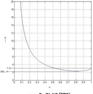
We definel= 2c, based on the conformal mapping Φa in (5), we know that αl = 2Φ1
0(a). Then we can plot a graphα/lversusaas in Figure 1.
Figure 1: α/lvsagraph
From the graph in Figure 1, we can see that for 2.300.. < α/l < π there exist two connected solution and that for α/l > πthere exists a unique solution (which is connected). Table 1 shows the number of the exact solutions of Problem 1.1 where µ as in (3). Although this table was shown in [2], we present it in more detailed form, particularly for the values α/l = 2.300... and α/l= 2.827.... According to [2], Ω is convex if and only if a≤1/√
3. We have αl = 2.827... for a= 1/√
3.
Table 1: Table of number of the solutions
α/l 0 ... 2.300... ... 2.827... ... π ...
# connected convex solution 0 0 0 0 1 1 1 1
# connected non-convex solution 0 0 1 2 1 1 0 0
# connected solution 0 0 1 2 2 2 1 1
# disconnected solution 0 1 1 1 1 1 0 0
Example of connected solutions are given in Figure 2 - 7 forα= 3, where we use MATLAB to draw them. We changeα/l= 2.3007,2.400,2.827,3.000, π,3.300. Then the number of solutions becomes 1,2,2,2,1,1 for each figure.
Figure 2: α/l= 2.300
Figure 3: α/l= 2.400
Figure 4: α/l= 2.827
Figure 5: α/l= 3.000
Figure 6: α/l=π
Figure 7: α/l= 3.300
3 Shape Optimization Approach
We consider Problem 1.1 withµas in (4). Then we replace µby
µ(x) =αδε(x−ξ1) +αδε(x−ξ2) (10) for sufficiently smallε <0, where
δε(x) :=
1
πε2 |x|< ε 0 |x| ≥ε.
We remark that the problems for µ=α(δc+δ−c) and for (10) are equivalent except for u(x) in D:=B(ξ1, ε)∪B(ξ2, ε).
We fixβ >0, and rewrite Problem 1.1 in the following equivalent form with a Robin boundary condition
−∆u=µ in Ω
u= 0 on Γ
βu+∂u
∂n =−1 on Γ.
We define
G:={Ω|Ω is a bounded domain inR2,D¯ ⊂Ω, ∂Ω : Lipschitz}.
Then for given Ω∈G with Γ =∂Ω, we can find a unique solutionuΩ∈H1(Ω) to the following problem
uΩ:
−∆u=µ in Ω βu+∂u
∂n =−1 on Γ.
IfuΩ= 0 on Γ then (uΩ,Ω) is a solution for Problem 1.1. Then we define a cost function as follows J(Ω) = 1
2 Z
Γ
|uΩ|2ds.
We want to minimizeJ(Ω) among Ω∈G. We remark here that (Ω, u) is a solution if and only if J(Ω) = 0 andu=uΩ.
4 Variation Formula of Cost Function
We use Lagrange multiplier method [5] to derive the variation formula of cost functionJ(Ω) with respect to the domain Ω∈G. For a vector field V∈W1,∞(R2,R2), we define
Ω(t) :={x+tV(x)
x∈Ω} (0≤t < t0).
Then we introduce an adjoint problem as follows vΩ:
∆v= 0 in Ω
βv+∂v
∂n =−uΩ on Γ.
By using the Lagrange multiplier method and the adjoint problem, under some regularity condi- tions, we obtain a variation formula of the cost function J(Ω):
d
dtJ(Ω(t)) t=0=
Z
Γ
(V·n)f+V· ∇g+ (Vs·τ)g
ds, (11)
whereτ is a counter clockwise tangential unit vector on Γ,Vs= ∂V∂τ, and f =∇uΩ· ∇vΩ
g=1
2u2Ω+αuΩvΩ+vΩ. A proof of (11) will be given in our forthcoming paper.
5 Traction Method
The main idea of traction method is to treat the domain Ω as an elastic body and iterate small deformation by a boundary traction given by the variational formula of J(Ω). In order to solve Problem 1.1 using the traction method, we have to solve the following artificial elasticity problem
−divσ[w] = 0 in Ω\D σ[w]n=−B on Γ
w= 0 on∂D,
(12)
wherew(x)∈R2is a displacement field on ¯Ω.
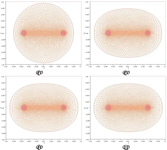
Figure 8: The initial domain We putB as boundary force, which is implicitly defined by
Z
Γ
B·V= d
dtJ(Ω(t)) = Z
Γ
(V·n)f +V· ∇g+ (Vs·τ)g
ds (∀V∈W1,∞(R2,R2)).
The complete procedure of solving Problem 1.1 by using the traction method can be summarized as follows:
1. Define an initial domain Ω as in figure (8) and generate a finite element mesh on Ω.
2. SolveuΩand vΩby finite element method.
3. Solve the artificial elasticity problem (12) by finite element method.
4. Modify the domain Ωnew :={x+ηw(x)|x∈Ω} for sufficiently small η > 0, together with the nodal points of the mesh.
5. Repeat step 2-4 until the domain Ω converges.
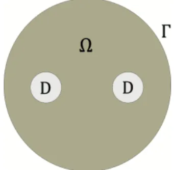
6 Numerical Examples
To study the efficiency of the traction method, we apply it into a free boundary problem as in Problem 1.1 withµas in (4). Figure 9 shows the numerical result of Problem 1.1 withα= 3 and c = 0.47727 (α/l=π) where we use FreeFem++ [3] for the simulation. We also summarize the value of the cost function for some iterations in Table 2.
Table 2: Table of the cost function
Iteration 500 1000 1500 2000 2500 2964
Cost function 0.00355... 0.000273... 0.0000541... 0.0000279... 0.0000218... 0.00000513...
From Table 2 we can see that the cost function becomes smaller with more iterations and it is almost equal to zero (J(Ω) = 0.00000513...) after 2964 iteration.
(a) (b)
(c) (d)
Figure 9: Numerical result of Problem 1.1 with α = 3 and c = 0.47727 (a) initial domain (b) iteration 1000 (c) iteration 2000 (d) iteration 2964
Comparing with the exact solution in Figure 6, we can observe that the numerical result after 2964 iteration in Figure 9 gives an accurate solution.
7 Conclusion
This paper has presented a complete construction of exact solutions of a free boundary problem by means of the conformal mapping based on the paper of A. Henrot [2]. We could classify all the exact solution into connected/disconnected and convex/non-convex ones and specified the number of each solutions for the case that µ is the combination of two Dirac function as shown in Theorem 2.2 and Table 1. The figures of some exact solutions are also presented in this paper using MATLAB. Hence we can use it as an comparison to the numerical result.
We also solved Problem 1.1 numerically using a shape optimization approach, specifically using the traction method. First we changed the free boundary problem in Problem 1.1 to a shape optimization problem as described in section 3. Then we derived the variation formula of the cost functionJ(Ω). Under some regularity, the variation formula in (11) could be obtained using the Lagrange multiplier method and the adjoint problem. The numerical result of Problem 1.1 (where
µ is a combination of two Dirac function with same coefficient α) for α/l =π obtained by the traction method was shown in Figure 9. It was observed that by comparing with the exact solution in Figure 6, the traction method could give the numerical result with good accuracy.
Acknowledgment
This research was made possible by Indonesian Directorate General of Higher Education (DGHE) scholarship. We are grateful to the DGHE for the scholarship which enabled one of the authors to undertake a Master double degree program at the Kanazawa University and Institut Teknologi Bandung. The authors also thank Dr. Michiaki Onodera, Kyushu University, who suggested us the reference [2].
References
[1] H. Azegami and K. Takeuchi (2006). A smoothing method for shape optimization: traction method using the robin condition.International Journal of Computational Methods, Vol. 3, No. 1, 21 – 33.
[2] A. Henrot (1994). Subsolutions and supersolutions in a free boundary problem. Ark. Mat., 32, 78 – 98.
[3] F. Hecht (2012). New development in FreeFem++. J. Numer. Math., 20, no. 3-4, 251265.
65Y15.
[4] D. Gilbarg and N. Trudinger (1998).Elliptic partial differential equations of second order.
Springer - Verlag, Berlin Heidelberg.
[5] J. Jahn (1996).Introduction to the theory of non-linear optimization. 2nd rev. ed.. Springer - Verlag, Berlin New York.