R ESEARCH I NSTITUTEFOR M ATHEMATICAL S CIENCESKYOTOUNIVERSITY,Kyoto,Japan BySatoruFUJISHIGE,Shin-ichiTANIGAWAandYuichiYOSHIDAMay2013 GeneralizedSkewBisubmodularity:ACharacterizationandaMin-MaxTheorem RIMS-1781

RIMS-1781

Generalized Skew Bisubmodularity:

A Characterization and a Min-Max Theorem

By

Satoru FUJISHIGE, Shin-ichi TANIGAWA and Yuichi YOSHIDA

May 2013

R _ESEARCH I NSTITUTE FOR M ATHEMATICAL S _CIENCES

Generalized Skew Bisubmodularity: A Characterization and a Min-Max Theorem

Satoru Fujishige^∗ Shin-ichi Tanigawa^† Yuichi Yoshida^‡ May 15, 2013

Abstract

Huber, Krokhin, and Powell (Proc. SODA2013) introduced a concept of skew bisubmodu- larity, as a generalization of bisubmodularity, in their complexity dichotomy theorem for valued constraint satisfaction problems over the three-value domain. In this paper we consider a nat- ural generalization of the concept of skew bisubmodularity and show a connection between the generalized skew bisubmodularity and a convex extension over rectangles. We also analyze the dual polyhedra, called skew bisubmodular polyhedra, associated with generalized skew bisub- modular functions and derive a min-max theorem that characterizes the minimum value of a generalized skew bisubmodular function in terms of a minimum-norm point in the associated skew bisubmodular polyhedron.

1 Introduction

For a finite setV let 2^V be the set of all subsets ofV and 3^V be the set of all the ordered pairs of disjoint subsets of V. A functionf : 3^V →R is calledbisubmodular if

f(X+, X₋) +f(Y+, Y₋)≥f(X+∩Y+, X₋∩Y₋) +f((X+∪Y+)\(X₋∪Y₋),(X₋∪Y₋)\(X+∪Y+)) for all (X+, X₋),(Y+, Y₋) ∈ 3^V. The concept of bisubmodularity was introduced in the study of ∆-matroids by Bouchet [3] and independently by Chandrasekaran–Kabadi [5] (also see [6, 1]).

Examples of ∆-matroids include the base family of a matroid as well as the family of matchable vertex sets in a graph, and bisubmodularity plays an important rˆole in combinatorial optimiza- tion for establishing the common generalization of matroid theory and matching theory from the optimization view point (see, e.g., [4]).

Bisubmodularity generalizes the well-known concept of submodularity. A function f : 2^V →R is called submodularif

f(X) +f(Y)≥f(X∪Y) +f(X∩Y)

∗Research Institute for Mathematical Sciences, Kyoto University, [email protected], Supported by JSPS Grant-in-Aid for Scientific Research (B) 25280004.

†Research Institute for Mathematical Sciences, Kyoto University, [email protected], Supported by JSPS Grant-in-Aid for Scientific Research (B) 25280004.

‡National Institute of Informatics, and Preferred Infrastructure, Inc.,[email protected], Supported by JSPS Grant-in-Aid for Research Activity Start-up (24800082), MEXT Grant-in-Aid for Scientific Research on Innovative Areas (24106001), and JST, ERATO, Kawarabayashi Large Graph Project.

for all X, Y ∈ 2^V. The Lov´asz extension fb(or the Choquet integral) of a submodular function f : 2^V → R is a convex extension over [0,1]^V, which plays a fundamental rˆole in minimizing submodular functions as well as generalizing the submodular analysis to discrete convex analysis.

In fact Gr¨otschel, Lov´asz, and Schrijver [13, Chapter 10] pointed out that one can minimize f by applying the ellipsoid method to fb, which led to the first weakly and strongly polynomial-time algorithms for minimizing submodular functions [12, 13]. Later, Iwata, Fleischer, and Fujishige [18] and Schrijver [22] independently gave combinatorial, strongly polynomial-time algorithms for minimizing submodular functions.

Algorithms for bisubmodular function minimization showed a similar historical development following submodular function minimization. Qi [21] proposed a convex extension of a bisubmod- ular function over [−1,1]^V and adapted the argument of Gr¨otschel, Lov´asz, and Schrijver [13] to bisubmodular functions. Fujishige and Iwata [10] extended their submodular function minimization algorithm to bisubmodular function minimization. The time complexity of their algorithm is not strongly polynomial, but later a combinatorial, strongly polynomial-time algorithm was developed by McCormick and Fujishige [20].

Huber, Krokhin, and Powell [17] introduced a generalization of bisubmodularity, called skew bisubmodularity, in their complexity dichotomy theorem for the valued constraint satisfaction prob- lems (VCSPs) over the three-value domain. Let α be a number with 0 < α ≤ 1. A function f : 3^V →Ris called α-bisubmodularif, for every X= (X+, X₋) andY = (Y+, Y₋)∈3^V,

f(X) +f(Y)≥f(X∩Y) +αf(X∪0Y) + (1−α)f(X∪1Y), (1) whereX∩Y= (X₊∩Y₊, X₋∩Y₋),X∪0Y= ((X₊∪Y₊)\(X₋∪Y₋),(X₋∪Y₋)\(X₊∪Y₊)), and X∪1Y= (X+∪Y+,(X₋∪Y₋)\(X+∪Y+)). 1-bisubmodularity is nothing but bisubmodularity.

A function f : 3^V → R is called skew bisubmodular if it is α-bisubmodular for some α ∈(0,1]. It was left open in the proceedings paper [17] to decide whether α-bisubmodular functions could be minimized in polynomial time for any α ∈ (0,1) in the value oracle model, but very recently we have been informed that Huber and Krokhin [16] showed that the minimization problem is indeed tractable via a convex extension.¹

In this paper we introduce a further natural generalization of the concept of skew bisubmodu- larity, and reveal the importance of (generalized) skew bisubmodularity from the point of view of discrete convex analysis. We examine an analog of the Lov´asz extension over generaln-dimensional rectangles and show that a necessary and sufficient condition for such an extension to be convex is the generalized skew bisubmodularity, where α-bisubmodularity introduced in [17] shows up as a special case when the rectangle is of form [−α,1]^V. This implies that the generalized skew bisub- modular functions can also be minimized in strongly polynomial time by the ellipsoid method. We also analyze the dual polyhedra, called skew bisubmodular polyhedra, associated with skew bisub- modular functions. It turns out that each orthant of a skew bisubmodular polyhedron forms a submodular polyhedron scaled by parameters, and skew bisubmodular polyhedra are special cases of polybasic polyhedra examined by Fujishige, Makino, Takabatake, and Kashiwabara [11]. Also skew bisubmodularity can be viewed as a special case of the discrete convexity defined within the general framework recently developed by Hirai [14, 15], while his general framework does not directly imply the oracle tractability of skew bisubmodular function minimization.

1The oracle tractability was announced at the Dagstuhl Seminar in November 2012 (see the slides of Anna Huber: VCSPs on Three Elements. Seminar 12451 on “The Constraint Satisfaction Problem: Complexity and Approximability”).

−α−(1)

−α−(2) α⁺(2)

α⁺(1)

Figure 1: The simplicial division of [−α⁻,α⁺] forn= 2.

Throughout the present paper we sometimes use bold-faced capital letters to denote elements in 3^V. For (X+, X₋) ∈3^V, for example, we use the bold-faced X to designate the pair (X+, X₋) and we define (X)+ =X+ and (X)₋=X₋. We adopt this convention for other letters as well. By X⊆Y we mean X₊ ⊆Y₊ andX₋⊆Y₋, and by X⊂Y we mean X⊆Y and X̸=Y.

For any X⊆V,χX denotes the characteristic vector of X inR^V.

Iff(∅,∅)̸= 0, one can apply arguments tof−f(∅,∅) instead off and derive the corresponding statements, so that we assume in the sequel that any function f : 3^V →Rsatisfiesf(∅,∅) = 0.

2 A Generalization of Skew Bisubmodularity

In this section we shall introduce an extension fbof a function f : 3^V → R over rectangles in Section 2.1 and then introduce generalized skew bisubmodular functions in Section 2.2. A relation between these two concepts is clarified in Section 3.

2.1 A simplicial division and an extension

For a finite set V of nelements let α= (α⁺,α⁻) be a pair of positive vectors α⁺,α⁻ :V →R>0

and consider the n-dimensional rectangle [−α⁻,α⁺] ={x∈R^V | −α⁻ ≤x≤α⁺}. For any X∈3^V define

χ^α_X= ∑

v∈X+

α⁺(v)χ_{v}− ∑

v∈X₋

α⁻(v)χ_{v}. (2) Then, for each chain A₁ ⊂ · · · ⊂ A_k in 3^V the convex hull of {χ^α_A

i |1 ≤i≤k} is a simplex and such simplices for all the maximal chains induce a simplicial division of rectangle [−α⁻,α⁺]. See Figure 1 for a two-dimensional example. This leads us to the the following essential fact.

Proposition 1. For any c ∈R^V \ {0}, there uniquely exist a chain (∅,∅) ̸=A1 ⊂ · · · ⊂ Ak and coefficientsλ1, . . . , λ_k∈R>0 such that

c=

∑k i=1

λ_iχ^α_Ai. (3)

By using the unique chainA₁⊂A₂ ⊂ · · · ⊂A_k and coefficientsλ₁, . . . , λ_k appearing in (3) for c∈R^V \ {0}, we define an extension fb:R^V →Rof a function f : 3^V →Rby

fb(c) =

∑k

i=1

λif(Ai) (c∈R^V \ {0}) (4)

and fb(0) =f(∅,∅) = 0.

2.2 Generalized skew bisubmodular functions

The key observation to analyze fbis a modular equation among the scaled characteristic vectors χ^α_X. This relation can be derived by checking howc≡χ^α_X+χ^α_Y can be expressed in the form of (3) forX,Y ∈3^V, i.e., we shall computeλ1, . . . , λk and A1 ⊂ · · · ⊂Ak for χ^α_X+χ^α_Y. The chain and coefficients can be written by an explicit formula by using binary operations∪t on 3^V fort∈(0,1) defined as follows: For each t∈(0,1) define

• Vt= (Vt,+, Vt,−)∈3^V by Vt,+ =

{

v∈V α⁻(v) α⁺(v) ≤t

}

, Vt,− = {

v∈V α⁺(v) α⁻(v) ≤t

}

• and a binary operation∪t on 3^V by

(X∪tY)+= (X∪0Y)+∪(Vt,+∩(X+∪Y+)∩(X₋∪Y₋)), (X∪tY)₋= (X∪0Y)₋∪(Vt,−∩(X+∪Y+)∩(X₋∪Y₋)).

Example. If V = {1,2,3,4}, _α^α−⁺⁽¹⁾(1) = ²₃, ^α_α⁺₋⁽²⁾₍₂₎ = ¹₃, ^α_α⁻+⁽³⁾(3) = ²₃, and _α^α−+⁽⁴⁾(4) = ¹₂, then V¹

3 = (∅,{2}), V¹

2 = ({4},{2}), V²

3 = ({3,4},{1,2}), and ({1,3},{2,4})∪0({2,4},{3}) = ({1},∅). We have ({1,3},{2,4})∪¹

3 ({2,4},{3}) = ({1},{2}), ({1,3},{2,4})∪¹

2 ({2,4},{3}) = ({1,4},{2}), and ({1,3},{2,4})∪²

3 ({2,4},{3}) = ({1,3,4},{2}).

Using ∪0 and ∪1 defined in Section 1, we have defined binary operations ∪t for all t ∈ [0,1].

Note thatVt⊆V_t′ ift≤t^′ and that these binary operations∪t are determined once we fixα.

We now have the following.

Lemma 2. For givenV andα, define a setT = {

min

{α⁻(v)

α⁺(v),^α_α⁺₋^(v)_(v)} v∈V

}∪{0,1}and arrange the distinct elements ofT in the increasing order of magnitude as0 =t0< t1< t2 <· · ·< tk+1 = 1.

Then we have

χ^α_X+χ^α_Y =χ^α_X∩Y+

∑k i=0

(ti+1−ti)χ^α_X∪tiY. (5) Proof. Denote the vector on the left-hand side of (5) by LH and that on the right-hand side by RH. We show LH(v) =RH(v) for allv∈V.

Choose any v∈V.

(I) If v /∈X₊∪X₋∪Y₊∪Y₋, then we haveLH(v) = 0 =RH(v).

(II) Ifv∈X₊∩Y₊, thenLH(v) = 2α⁺(v). Sincev∈X₊∩Y₊andv∈(X∪0Y)₊⊆(X∪tiY)₊ for all i, we also have RH(v) = 2α⁺(v).

(III) If v ∈ X+\(Y+ ∪Y₋), then LH(v) = α⁺(v). Since v /∈ (X∩Y)+∪(X∩Y)₋ and v∈(X∪0Y)₊ ⊆(X∪tiY)₊ for all i, we also have RH(v) =α⁺(v).

(IV) Because of the symmetry we assume that the remaining case is when v ∈ X₊ ∩Y₋. Then, LH(v) = α⁺(v)−α⁻(v). Suppose that α⁺(v) ≥ α⁻(v). Then, v /∈ (X∪tY)₋ for any t∈[0,1), andv ∈(X∪tY)₊ if and only if ^α_α⁻+^(v)(v) ≤t. By definition, there is an index j such that tj = ^α_α⁻+^(v)(v). Sincev /∈(X∩Y)+∪(X∩Y)₋, we thus have RH(v) =∑_k

i=0(ti+1−ti)χ^α_X∪

tiY(v) =

∑_k

i=j(t_i+1−t_i)χ^α_X∪

tiY(v) =∑_k

i=j(t_i+1−t_i)α⁺(v) = (t_k+1−t_j)α⁺(v) =α⁺(v)−α⁻(v) =LH(v).

The same argument can also be applied to the case when α⁺(v)<α⁻(v).

This completes the proof.

Motivated by Lemma 2, we say that a functionf : 3^V →R isα-bisubmodularif f(X) +f(Y)≥f(X∩Y) +

∑k

i=0

(ti+1−ti)f(X∪tiY) (6) for all X,Y∈3^V, wheret_i (i= 0, . . . , k+ 1) are those defined in Lemma 2. Whenα⁺(v) = 1 and α⁻(v) =α for allv∈V for some α∈(0,1],α-bisubmodularity becomesα-bisubmodularity in [17]

defined by (1).

3 Skew Bisubmodular Polyhedron and Convexity of f b

Let α = (α⁺,α⁻) with α⁺ :V → R>0 and α⁻ :V → R>0. For any x ∈R^V and X ∈3^V define x(χ^α_X) =∑

v∈V x(v)χ^α_X(v), which is the canonical inner product⟨x, χ^α_X⟩ ofx andχ^α_Xin (2). Hence, x(χ^α_X) = ∑

v∈X+

α⁺(v)x(v)− ∑

v∈X₋

α⁻(v)x(v). (7)

Also define the α-bisubmodular polyhedronP(f) associated with anα-bisubmodular function f by P(f) ={x∈R^V | ∀X∈3^V :x(χ^α_X)≤f(X)}. (8) We show that fb defined by (4) is the support function of P(f), i.e., for any c ∈ R^V, fb(c) = max{⟨c, x⟩ |x ∈P(f)}. This implies that α-bisubmodularity is a necessary and sufficient condi- tion for the convexity of fb(Theorem 7 shown below). The argument given here is essentially an adaptation of bisubmodular analysis given in [9].

Let us proceed to the detailed description. For any given c∈R^V consider the following linear programming problem.

(P) Maximize ⟨c, x⟩ subject to x∈P(f).

To show that a dual optimal solution of this problem forms a chain, we first consider a relaxation of the system of linear inequalities defining P(f) in (8).

A pair S = (S₊, S₋) ∈ 3^V is called an orthant if S₊ ∪S₋ = V. The set of all the pairs X= (X₊, X₋) such thatX₊⊆S₊ and X₋ ⊆S₋ is denoted by 2^S. We define a superset P_S(f) of P(f) by

P_S(f) ={x∈R^V | ∀X∈2^S:x(χ^α_X)≤f(X)}, which is obtained from P(f) by discarding constraints not related to 2^S.

The advantage of introducing orthants is that the maximization over P_S(f) is equivalent to the maximization over a submodular polyhedron. Let us explain this fact now. Notice that, once we fix an orthant S,f becomes submodular on 2^S. In other words, by definingfS: 2^V →Rby

f_S(X) =f(S₊∩X, S₋∩X) (X ⊆V),

f_S is submodular on 2^V. Consider the submodular polyhedron P(f_S), which is given by P(f_S) ={x∈R^V | ∀X⊆V:x(X)≤f_S(X)}.

Then, observe

P_S(f) ={x∈R^V | ∃y∈P(f_S),∀v∈S+:α⁺(v)x(v) =y(v),∀v∈S₋: −α⁻(v)x(v) =y(v)}. This implies that P_S(f) can be obtained from P(f_S) by reflections and scaling along axes, and P_S(f) is combinatorially equivalent to P(f_S). Recall that a greedy algorithm solves the maximization problem over any submodular polyhedron (see [7, 9]). In terms of PS(f) we obtain a variant of the greedy algorithm, Greedy Algorithm, which actually computes an optimal solution of (P) together with the relevant orthantS (see Theorem 5 shown below).

Greedy Algorithm

Input: An α-bisubmodular function f : 3^V →R+ on a finite set V, and a vector c∈R^V. Output: An optimal solutionx^∗ of (P).

1: Compute an orthantS= ({v∈V |c(v)≥0},{v∈V |c(v)<0}) and a vector c_α∈R^V by cα(v) =

{ _c(v)

α⁺(v) ifv∈S₊

−_α^c(v)−(v) ifv∈S₋ (v∈V). (9)

2: Find a total orderingL= (v1, v2, . . . , vn) of V such thatcα(v1)≥cα(v2)≥ · · · ≥cα(vn).

3: Compute a vector x^∗∈R^V by x^∗(v_i) =

{ ₁

α⁺(vi)(f(X_i)−f(X_i−1)) ifv_i∈S₊

−_α−¹(vi)(f(X_i)−f(X_i−1)) ifv_i∈S₋ (1≤i≤n), (10) whereXi is the restriction of Sto{v1, . . . , vi} andX0= (∅,∅).

4: Return x^∗.

Proposition 3. Let f : 3^V →R be an α-bisubmodular function. For c∈R^V, let x^∗ be the vector and S be the orthant computed by Greedy Algorithm. Then x^∗ is an extreme point of

BS(f) :={x∈R^V |x∈PS(f), x(χ^α_S) =f(S)}, and ⟨c, x^∗⟩ ≥ ⟨c, x⟩ for all x∈PS(f).

Following the argument in [9, Section 3.5(b)], we now show thatx^∗is indeed an optimal solution not only over P_S(f) but also over P(f). To see this we need one more technical lemma, which is an analogue of [9, Lemma 3.60] for bisubmodular analysis.

Lemma 4. Let f : 3^V → R be an α-bisubmodular function. For each orthant S ∈ 3^V we have BS(f)⊆P(f).

Proof. Let x ∈ B_S(f). It then follows from α-bisubmodularity of f and Lemma 2 that for any X∈3^V we have

x(χ^α_X)−f(X)

=x(χ^α_X)−f(X) +x(χ_S^α)−f(S) (byx∈B(f))

≤x(χ^α_X∩S) +

∑k i=0

(ti+1−ti)x(χ^α_X∪tiS)−[f(X∩S) +

∑k i=0

(ti+1−ti)f(X∪tiS)]

≤0 (by x∈P(f)), which impliesx∈P(f).

Theorem 5. Let f : 3^V → R be an α-bisubmodular function. For c ∈ R^V, let x^∗ be the vector obtained by Greedy Algorithm. Then we have ⟨c, x^∗⟩ ≥ ⟨c, x⟩ for all x∈P(f).

Proof. LetS= ({v∈V |c(v)≥0},{v∈V |c(v)<0}) be the orthant computed byGreedy Algorithm.

Note that P(f)⊆P_S(f). Combining this relation with Lemma 4, we have

max{⟨c, x⟩ |x∈P_S(f)} ≥max{⟨c, x⟩ |x∈P(f)} ≥max{⟨c, x⟩ |x∈B_S(f)}.

However, Proposition 3 implies max{⟨c, x⟩ | x∈ P_S(f)} = max{⟨c, x⟩ |x ∈ B_S(f)}=⟨c, x^∗⟩. We thus have ⟨c, x^∗⟩ ≥ ⟨c, x⟩ for anyx∈P(f).

Corollary 6. Let f : 3^V →R be anα-bisubmodular function. Then, for any c∈R^V we have fb(c) = max{⟨c, x⟩ |x∈P(f)} (c∈R^V). (11) Proof. Let vectorscαandx^∗and chainX1 ⊂X2⊂ · · · ⊂Xnbe those computed byGreedy Algorithm.

Define λi by λi =cα(vi)−cα(vi+1) for 1 ≤i≤k−1 and by λ_k = cα(v_k). Then it can easily be checked that ⟨c, x^∗⟩ = ∑_n

i=1λ_if(X_i) and c = ∑_n

i=1λ_iχ^α_X

i. Therefore, we obtain (11) because of Proposition 1, the definition of fb, and Theorem 5.

We now show a main theorem of this section. We remark that, from the definition of fbin (4), fbis positively homogeneous(i.e.,fb(λc) =λfb(c) for anyλ >0 andc∈R^V).

Theorem 7. Let V be a finite set and α = (α⁺,α⁻) be a pair of vectors α⁺ : V → R>0 and α⁻ :V →R>0. Then, for any f : 3^V →R, fbis convex if and only if f is α-bisubmodular.

Proof. The proof is essentially the same as that of the corresponding theorem for submodular functions given in [9, Theorem 6.13]. Let us give it for the sake of completeness.

For each c∈R^V, letx_cbe a maximizer of the right-hand side of (11). Then, for any c, c^′ ∈R^V, we have 2f(b ^c+c₂^′) =fb(c+c^′) = ⟨c+c^′, xc+c^′⟩ ≤ ⟨c, xc⟩+⟨c^′, xc^′⟩=fb(c) +fb(c^′), which implies the convexity offb.

Conversely, suppose that fbis convex. To show α-bisubmodularity of f, take any X and Y in 3^V. Since fbis positively homogeneous and convex, we have

f(χb ^α_X+χ^α_Y)

2 =fb

(χ^α_X+χ^α_Y 2

)

≤ fb(χ^α_X) +fb(χ^α_Y)

2 . (12)

On the other hand, since X∩Y ⊆ X∪t0 Y ⊆ X∪t1 Y ⊆ · · · ⊆ X∪tk Y, it follows from the definition offbin (4) that

fb (

χ^α_X∩Y+

∑k i=0

(t_i+1−t_i)χ^α_X∪

tiY

)

=fb(χ^α_X∩Y) +

∑k i=0

f((tb _i+1−t_i)χ^α_X∪

tiY). (13)

Therefore,

f(X) +f(Y) =f(χb ^α_X) +fb(χ^α_Y) (sincefbis an extension of f)

≥fb(χ^α_X+χ^α_Y) (by (12))

=fb (

χ^α_X∩Y+

∑k i=0

(t_i+1−t_i)χ^α_X∪

tiY

)

(by (5))

=f(χb ^α_X∩Y) +

∑k i=0

fb((t_i+1−t_i)χ^α_X∪

tiY) (by (13))

=f(χb ^α_X∩Y) +

∑k i=0

(ti+1−ti)fb(χ^α_X∪tiY) (since fbis positively homogeneous)

=f(X∩Y) +

∑k i=0

(t_i+1−t_i)f(X∪tiY) (since fbis an extension off) Hence f isα-bisubmodular.

We also have the following theorem (see [2, 17] for special cases of bisubmodular and α- bisubmodular functions; also see [14, Proposition 4.11] for more general functions).

Theorem 8. Under the same assumption as in Theorem 7, f : 3^V →R is α-bisubmodular if and only if

(a) for every orthant S, f restricted on 2^S is submodular, and

(b) for everyv∈V and U ⊆V \ {v}, puttingW =V \({v} ∪U), we have

α⁻(v)f(U∪ {v}, W) +α⁺(v)f(U, W∪ {v})≥(α⁺(v) +α⁻(v))f(U, W).

Proof. We can easily see that the α-bisubmodularity of f implies (a) and (b). Hence it suffices to show the if part.

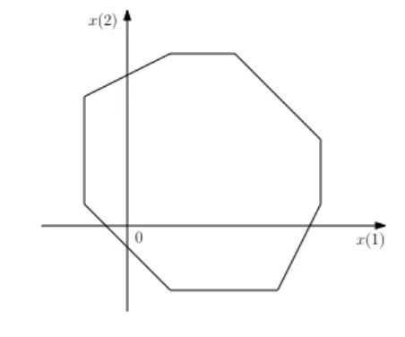
Suppose that (a) and (b) hold. It follows from (a) that the extensionfbdefined by (4) is convex on the cone R^S_≥⁺₀×R_≤^S−₀ of every orthantS (see [19]). Moreover, (b) implies the convexity of fbon

0 x(2)

x(1)

Figure 2: A ¹₂-bisubmodular polyhedron.

the union of adjacent simplices (having common facetx(v) = 0) that correspond to maximal chains of 3^V:

X0(= (∅,∅))⊂ · · · ⊂Xn−1(= (U, W))⊂Xn= (U ∪ {v}, W), X0(= (∅,∅))⊂ · · · ⊂Xn−1(= (U, W))⊂X^′_n= (U, W ∪ {v}),

where note that only the last elements (adjacent orthants) are different. Hencefbis convex, so that f is α-bisubmodular due to Theorem 7.

For a submodular function f : 2^V →R, letfbbe the Lov´asz extension off ([19]). As shown by Gr¨otschel, Lov´asz, and Schrijver [13], one can develop a polynomial-time (weak) separation oracle that separates a point p ∈R^V \F from the set F of minimizers of fb, which implies that one can find a minimizer of fbin polynomial time. Since fbis linear on each cell of the simplicial division, one can also find a minimizer off. Qi [21] extended this argument to bisubmodular functions, and here we can adopt the same argument forα-bisubmodular function f due to the convexity offb. Corollary 9. Any α-bisubmodular function f : 3^V →R can be minimized in strongly polynomial time.

It follows from Proposition 3 and Theorem 5 that, for a fixed orthant S, P_S(f) is the one obtained from a submodular polyhedron by a reflection and scaling. It is known that each edge vector (i.e., a direction vector of each edge) of a bisubmodular polyhedron is one of the following forms

(0, . . . ,0,1,0. . . ,0), (0, . . . ,0,±1,0, . . . ,0,∓1,0, . . . ,0), (0, . . . ,0,±1,0, . . . ,0,±1,0, . . . ,0) and hence each edge vector of anα-bisubmodular polyhedron has the support of size at most two.

See Figure 2 for an example.

The concept of a polybasic polyhedron is introduced in [11], where a convex polyhedron is polybasic if every edge vector has a support of size at most two. Hence, skew bisubmodular polyhedra are special cases of polybasic polyhedra.

4 A Min-Max Theorem

For anyx∈R^V let us define

∥x∥α= ∑

v∈V:x(v)>0

α⁻(v)x(v)− ∑

v∈V:x(v)<0

α⁺(v)x(v).

It is not difficult to see that∥·∥αis a norm onR^V. The following extension of a theorem given in [8]

implies that theα-bisubmodular function minimization can be reduced to finding a minimum-norm point with respect to∥ · ∥α in theα-bisubmodular polyhedron P(f).

To show this we need one technical lemma. For x∈P(f),X is called x-tightifx(χ^α_X) =f(X).

Lemma 10. Letx∈P(f). If Xand Y are x-tight, thenX∩Y and X∪tiY (i= 0, . . . , k+ 1) are alsox-tight.

Proof. By using Lemma 2, x∈P(f),α-bisubmodularity off, and thex-tightness of Xand Y, we havex(χ^α_X)+x(χ^α_Y) =x(χ^α_X∩Y)+∑_k

i=0(ti+1−ti)x(χ^α_X∪

tiY)≤f(X∩Y)+∑_k

i=0(ti+1−ti)f(X∪tiY)≤ f(X) +f(Y) =x(χ^α_X) +x(χ^α_Y). Hence, the inequalities must hold with equality, from which follows the present lemma.

Theorem 11. For any α-bisubmodular function f : 3^V →R,

min{∥x∥α|x∈P(f)}= max{−f(X)|X∈3^V}. (14) Proof. For any x∈P(f) and X= (X₊, X₋)∈3^V, we always have ∥x∥α≥ −f(X) since

∥x∥α= ∑

v∈V:x(v)>0

α⁻(v)x(v)− ∑

v∈V:x(v)<0

α⁺(v)x(v)≥ ∑

v∈X−

α⁻(v)x(v)− ∑

v∈X+

α⁺(v)x(v)≥ −f(X).

Hence it suffices to show that ∥x∥α=−f(X) for some x∈P(f) and X∈3^V.

Let ˆx be a minimizer of the left-hand side of (14), and letA₊={v∈V |x(v)ˆ <0},A₋ ={v∈ V |x(v)ˆ >0}, and A = (A+, A₋). Note that for any u ∈ A+ and v ∈A₋ there exist ˆx-tight X and Y such thatu∈X+ and v∈Y₋.

Take any u∈A₊. For each v ∈A₋, if every ˆx-tight X withu∈X₊ satisfiesv ∈X₊, then for a sufficiently small positive number ϵ, we can obtain a better solution than ˆx in the minimization problem by increasing ˆx(u) byϵ/α⁺(u) and decreasing ˆx(v) byϵ/α⁺(v). Therefore, for eachv∈A₋, there exists an ˆx-tightX^uv such thatu∈X₊^uvand v /∈X₊^uv. Similarly, for eachv∈A₊\ {u}, there exists an ˆx-tight set X^uv such thatu∈X₊^uv and v /∈X₋^uv, since otherwise (i.e., no such ˆx-tight set exists) for a sufficiently small positive number ϵ, increasing ˆx(u) byϵ/α⁺(u) and ˆx(v) by ϵ/α⁻(v) gives a better solution again. Put X^u =∩

v∈(A+\{u})∪A₋X^uv. It follows from Lemma 10 that X^u is ˆx-tight withu∈X₊^u,X₊^u ∩A₋=∅, and X₋^u ∩A+ =∅.

By a symmetric argument we see that for anyu∈A₋ there is an ˆx-tightX^u such thatu∈X₋^u, X₊^u ∩A₋=∅, and X₋^u ∩A₊=∅.

PutX^∗=∪

0X^u, where∪0 is taken over allu∈A₊∪A₋. Then, it follows from Lemma 10 that X^∗ is ˆx-tight with A+⊆X₊^∗ andA₋⊆X₋^∗. Moreover, since ˆx(v) = 0 for allv∈V \(A+∪A₋) by

the definition of A₊ and A₋, we have

∥xˆ∥α= ∑

v∈V:ˆx(v)>0

α⁻(v)ˆx(v)− ∑

v∈V:ˆx(v)<0

α⁺(v)ˆx(v) = ∑

v∈A₋

α⁻(v)ˆx(v)− ∑

v∈A+

α⁺(v)ˆx(v)

= ∑

v∈X₋^∗

α⁻(v)ˆx(v)− ∑

v∈X₊^∗

α⁺(v)ˆx(v) =−x(χˆ ^α_X∗)

Consequently, by the ˆx-tightness of X^∗, we obtain ∥xˆ∥α = −x(χˆ ^α_X∗) = −f(X^∗). This completes the proof.

5 Concluding Remarks

We have considered a natural generalization of the concept of skew bisubmodularity. We have shown a characterization of the generalized skew bisubmodularity in terms of its convex extension over rectangles, where an important rˆole is played by skew bisubmodular polyhedra associated with skew bisubmodular functions. We have also derived a min-max theorem (Theorem 11) that relates the minimum value of a skew bisubmodular function to a minimum-norm point in the associated skew bisubmodular polyhedron. All the existing combinatorial algorithms for minimizing submodular functions or bisubmodular functions are based on min-max theorems corresponding to Theorem 11.

Devising a combinatorial polynomial-time algorithm for skew bisubmodular function minimization will be discussed elsewhere.

References

[1] K. Ando and S. Fujishige: On structures of bisubmodular polyhedra.Mathematical Program- ming, 74:293–317 (1996).

[2] K. Ando, S. Fujishige and T. Naitoh: A characterization of bisubmodular functions. Discrete Mathematics, 148:299–303 (1996).

[3] A. Bouchet. Greedy algorithm and symmetric matroids. Mathematical Programming, 38(2):147–159, 1987.

[4] A. Bouchet and W. H. Cunningham. Delta-matroids, jump systems, and bisubmodular poly- hedra. SIAM Journal on Discrete Mathematics, 8(1):17–32, 1995.

[5] R. Chandrasekaran and S. N. Kabadi. Pseudomatroids. Discrete Mathematics, 71(3):205–217, 1988.

[6] F. D. J. Dunstan and D. J. A. Welsh. A greedy algorithm for solving a certain class of linear programmes.Mathematical Programming, 62: 338–353, 1973.

[7] J. Edmonds. Submodular functions, matroids, and certain polyhedra. Proceedings of the Cal- gary International Conference on Combinatorial Structures and Their Applications (R. Guy, H. Hanani, N. Sauer and J. Sch¨onheim, eds., Gordon and Breach, New York, 1970), pp. 69–87;

also in: Combinatorial Optimization—Eureka, You Shrink! (M. J¨unger, G. Reinelt and G.

Rinaldi, eds., Lecture Notes in Computer Science2570, Springer, Berlin, 2003), pp. 11–26.

[8] S. Fujishige. A min–max theorem for bisubmodular polyhedra. SIAM Journal on Discrete Mathematics, 10(2):294–308, 1997.

[9] S. Fujishige. Submodular Functions and Optimization, volume 58 ofAnnals of Discrete Math- ematics. Elsevier, 2nd edition, 2005.

[10] S. Fujishige and S. Iwata. Bisubmodular function minimization. SIAM Journal on Discrete Mathematics, 19(4):1065–1073, 2005.

[11] S. Fujishige, K. Makino, T. Takabatake, and K. Kashiwabara. Polybasic polyhedra: structure of polyhedra with edge vectors of support size at most 2. Discrete Mathematics, 280(1):13–27, 2004.

[12] M. Gr¨otschel, L. Lov´asz, and A. Schrijver. The ellipsoid method and its consequences in combinatorial optimization. Combinatorica, 1(2):169–197, 1981.

[13] M. Gr¨otschel, L. Lov´asz, and A. Schrijver. Geometric Algorithms and Combinatorial Opti- mization, volume 2 of Algorithms and Combinatorics. Springer-Verlag, 1st edition, 1988.

[14] H. Hirai. Discrete convexity and polynomial solvability in minimum 0-extension problems.

Mathematical Engineering Technical Reports, METR 2012-18, Department of Mathematical Informatics, Graduate School of Information Science and Technology, The University of Tokyo, October 2012.

[15] H. Hirai. Discrete convexity for multiflows and 0-extensions.Proceedings of the 8th Japanese- Hungarian Symposium on Discrete Mathematics and Its Applications, June 4-7, 2013 in Veszpr´em, Hungary.

[16] A. Huber and A. Krokhin. A Lov´asz extension for skew bisubmodular functions. Unpublished manuscript, October 30, 2012.

[17] A. Huber, A. Krokhin, and R. Powell. Skew bisubmodularity and valued CSPs. InSODA’13:

Proceedings of the 24th Annual ACM-SIAM Symposium on Discrete Algorithms, pages 1296–

1305, 2013.

[18] S. Iwata, L. Fleischer, and S. Fujishige. A combinatorial strongly polynomial algorithm for minimizing submodular functions. Journal of the ACM, 48(4):761–777, 2001.

[19] L. Lov´asz.: Submodular functions and convexity. In: Mathematical Programming—The State of the Art(A. Bachem, M. Gr¨otschel and B. Korte, eds., Springer, Berlin, 1983), pp. 235–257.

[20] S. T. McCormick and S. Fujishige. Strongly polynomial and fully combinatorial algorithms for bisubmodular function minimization. Mathematical Programming, 122(1):87–120, 2008.

[21] L. Qi. Directed submodularity, ditroids and directed submodular flows. Mathematical Pro- gramming, 42(1-3):579–599, 1988.

[22] A. Schrijver. A combinatorial algorithm minimizing submodular functions in strongly polyno- mial time. Journal of Combinatorial Theory, Series B, 80(2):346–355, 2000.