Finite element methods for nearly incompressible media (Mathematical Analysis of Viscous Incompressible Fluid)

Finite

element methods for nearly incompressible

media

Fumio

Kikuchi*

Professor

Emeritus,

The

University of Tokyo

Abstract

Wewillsummarizeandanalyzesomefinite element methods for analysis of nearly

orcompletely incompressible mediaincludinglinearly elastic solids andviscous

New-tonianfluids. Numerical analysis of such problemsisdifficultespeciallyinselecting

ap-propriate finite elementmodels, and the mixedFEM anddiscontinuous Galerkin FEM

(DG FEM) areofteneffectivetoobtain reliable numerical solutions.

1

Introduction

We will present

some

finite element methods for analysis of nearly (or completely)

incom-pressible media including elastic solids andviscousfluids. Numerical analysis of such

prob-lems is difficult especially in selecting appropriate finite element models. Especially, the

genuine methods based

on

displacements

or

velocities only usually suffer from

volumet-ric locking in the nearly incompressible range,

so

that various attempts have been made.

Among them, the mixed and the stabilization methods

are

known to be effective in this

re-spect. Nowadays, the discontinuous Galerkin methods combined with the mixed methods

become to be realized to be

more

effective to obtain reliable numerical solutions. In this

note,

we

will summarize

some

knownresults

as

well

as our

own ones.

Acknowledgment: The present authorexpresses his sincere thanks toDr. Daisuke Koyama

ofUniversity ofElectro-Communications

as

ajoint workerofthis report for the section on

plain strain problems.

2

Nearly incompressible

media

We will mainly discuss the solid

cases

below. Let $x=\{x_{1}, x_{N}\}(N=2,3)$ denote the

Cartesiancoordinates, and$\Omega\subset \mathbb{R}^{N}$

be

a

bounded domain occupied by the solid. We will

use

the notation of small displacements of solids

as

$u=\{u_{i}\}_{1\leq i\leq N}$, and the associated small

or

linearized strains

as

$e_{ij}(u)=(\partial_{j}u_{i}+\partial_{i}u_{j})/2 (\partial_{i}=\partial/\partial x_{i};1\leq i, j\leq N)$, (1) $*E$-mail address: _{[email protected]}

which

can

be regarded

as a

second-order symmetric tensor. The diagonal components $e_{ii}$

are

normal stretching strains, while the off-diagonal

ones

$e_{ij}(i\neq])$

are

shearing strains.

Moreover, the volumetric strain is given by$divu=\sum_{i=1}^{N}e_{ii}(u)$,whichplays importantroles

innearlyincompressible

cases.

Remark 1 For$N=2$,we assume that the

_functions

donotdepend

on

$x_{3}$and also that$u_{3}=0$

(inthe$3D$notations), so that$e_{33}=e_{i3}=e_{i3}=0(i=1,2)$

.

The stresses $s_{ij}(1\leq i, j\leq 3)$

are

also treated

as a

second-order symmetrictensor, and

we

assume

the followinggeneralizedHooke’s law forisotropic solids:

$s_{ij}(u)=\lambda(divu)\delta_{ij}+2\mu e_{ij}(u)$ $(\lambda>0, \mu>0 : Lam\’{e}$’sparameters)

.

(2)

Noticethat $s_{33}$ maynotvanishunder the above relation. We will

assume

in additionthatthe

solidishomogeneous, thatis, $\lambda$ and

$\mu$donotdependon $x.$

The static

pressure

isdefined by theminus of

mean

normal stress, thatis,

$p:=- \frac{1}{3}\sum_{i=1}^{3}s_{ii}=-(\lambda+\frac{2\mu}{3})divu\Rightarrow$ $s_{ij}=- \frac{\lambda}{\lambda_{B}}p+2\mu e_{ij}(u)(\lambda_{B}:=\lambda+2\mu/3)$, (3)

where$\lambda_{B}$ iscalled the bulkmodulus, and,

as

was

noted,theterm $s_{33}$ is

necessary.

The above

suggests that$divuarrow 0$

as

$\lambdaarrow+\infty$

.

(Under

appropriate

settings,

we

can

also show$parrow p_{\infty}$

for

some

$p_{\infty}.$) In

some

mathematicalliteratures, $p$is simply defined by $p=-\lambda divu$

.

Such

anonphysical definition maybe

more

convenientforpuremathematical analysis.

The staticequilibrium ofstresses isexpressed by the following Cauchy equations:

$- \sum_{j=1}^{N}\partial s_{ij}/\partial x_{j}=f_{i} (1\leq i\leq N)$, (4)

where $f=\{f\}_{1\leq i\leq N}$ isthe distributed body forcevector. Substituting (1) and (2) into(4),

we

have Navier’s equations forisotropic homogeneous solids:

$- \lambda\partial_{i}divu-\mu\sum_{j=1}^{N}\partial_{j}(\partial_{j}u_{i}+\partial_{i}u_{j})=f(1\leq i\leq N)$, (5)

(by (3)) $\Rightarrow$ $\frac{\lambda}{\lambda_{B}}\partial_{i}p-\mu\sum_{j=1}^{N}\partial_{j}(\partial_{j}u_{i}+\partial_{i}u_{j})=f_{i}(1\leq i\leq N)$

.

(6)

3

Weak

formulations

For simplicity,

we

will consider the

pure

homogeneous Dirichlet boundary conditions, and

use

the usual Hilbertian Sobolev spaces $H^{1}(\Omega)$ and $H_{0}^{1}(\Omega)$

.

We will also denote the inner

products of$L^{2}(\Omega)$

or

$L^{2}(\Omega)^{N}$by $)_{\Omega}$ and their associated

norms

by $||\cdot||_{\Omega}$

.

Below

we

will

3.1

Displacement

formulation in

$u$

only

The most fundamental weak formulation for finite $\lambda>0$ is the following

one

using the

displacementonly.

[DF] Given$f\in L^{2}(\Omega)$_, find$u\in H_{0}^{1}(\Omega)^{N}$ thatsatisfies

$\lambda(divu, divv)_{\Omega}+2\mu\sum_{i,j=1}^{N}(e_{ij}(u), e_{ij}(v))_{\Omega}=(f, v)_{\Omega}(\forall v\in H_{0}^{1}(\Omega)^{N})$

.

(7)

For mathematical analysis ofthe above formulation, Korn’s inequalities

are

essential,

and

a

typical example of them is: There exists

a

domain constant$C>0$suchthat

$\sum_{i,j=1}^{N}||e_{ij}(v)||_{\Omega}^{2}+\Vert v\Vert_{\Omega}^{2}\geq C||v\Vert_{H^{1}(\Omega)^{N}}^{2}(\forall v\in H^{1}(\Omega)^{N})$

.

(8)

The presentresult is generalized to the Sobolev

space

$W^{1,p}(\Omega)$ with _$1<p<\infty$ for$N=2$

[17]. For$v\in H_{0}^{1}(\Omega)^{N}$,the above becomes$\sum_{i,j=1}^{N}||e_{ij}(v)||_{\Omega}^{2}\geq C||v||_{H^{1}(\Omega)^{N}}^{2}$ withpossible change

of$C>0$, from which

we

can

conclude theexistence anduniqueness of the weak solution $u$

of[DF]. Moreover, keeping$\mu$ constant,

we

have$\lambda||divu||_{\Omega}^{2}\leq C||f\Vert_{\Omega}^{2}$,

so

that$divuarrow 0$ in

$L^{2}(\Omega)$

as

$\lambda$

tends to$+\infty.$

3.2

Mixed

formulation in

$u$

and

_$p$

To deal with the nearly and completely incompressible cases, _{it is} natural to add $p$

as

an

independent unknown function.

[MF] Given$f\in L^{2}(\Omega)$,find $\{u, p\}\in H_{0}^{1}(\Omega)^{N}\cross L^{2}(\Omega)$ thatsatisfies

$\{\begin{array}{ll}2\mu\sum_{i,j=1}^{N}(e_{ij}(u), e_{ij}(v))_{\Omega}-\frac{\lambda}{\lambda_{B}}(p,divv)_{\Omega}=(f, v)_{\Omega} (\forall v\in H_{0}^{1}(\Omega)^{N}) ,- \frac{\lambda}{\lambda_{B}}[(divu, q)_{\Omega}+\lambda_{B}^{-1}(p, q)_{\Omega}]=0 (\forall q\in L^{2}(\Omega)) .\end{array}$ (9)

We

can see

formally that$p$is the Lagrange multiplier for the linear constraint$p+\lambda_{B}divu=0.$

Also, bythe Gaussformula,

we

find that$p\in L_{0}^{2}(\Omega)$ for$L_{0}^{2}(\Omega)=\{q\in L^{2}(\Omega);(q, 1)_{\Omega}=0\}.$

To deal with [MF], it is essential to

use

the following inf-sup condition: There exists $a$

constant$K>0$ _{such that}

$inf\sup \underline{(divv,q)_{\Omega}}\geq K$

_.

(10)

$v\in H_{0}^{1}(\Omega)^{N}\backslash \{0\}_{q\in L_{0}^{2}(\Omega)\backslash \{0\}}||v||_{H^{1}(\Omega)^{N}}\cdot||q||_{\Omega}$

Thiscondition isrelated to the solvabilityof$divv=g\in L_{0}^{2}(\Omega)$for$v\in H_{0}^{1}(\Omega)^{N}.$

Usingthe above,

we

can

conclude the existence anduniqueness of$\{u,p\}$with

$||u\Vert_{H^{1}(\Omega)^{N}}+||p||_{\Omega}\leq C||f||_{\Omega}$ uniformly in $\lambda\geq\lambda_{0}=$ positiveconstant. (11)

Moreover,

as

$\lambda$ tends to

$\infty,$ $\{u,p\}$

converges

strongly in $H_{0}^{1}(\Omega)^{N}\cross L^{2}(\Omega)$ to

a

$\{u_{\infty}, p_{\infty}\}\in$ $H_{0}^{1}(\Omega)^{N}\cross L_{0}^{2}(\Omega)$,which satisfies [MF]formally with $\lambda/\lambda_{B}=1$ and$\lambda_{B}^{-1}=0$

:

$\{\begin{array}{l}2\mu\sum_{i,j=1}^{N}(e_{ij}(u_{\infty}), e_{ij}(v))_{\Omega}-(p_{\infty},divv)_{\Omega}=(f, v)_{\Omega}(\forall v\in H^{1}(\Omega)^{N}) ,-(divu_{\infty}, q)_{\Omega}=0(\forall q\in L^{2}(\Omega)) \cdots\cdots incompressibility condition.\end{array}$ (12)

ForFrierdrichs-Kellermeshes,

kernel

_of

$div|_{(V_{0}^{h})^{2}}$

for

$k=1$ is$\{0\}.$

Figure 1: Triangular meshes of Frierdrichs-Keller type for

a square

domain

4

FEM based

on

[DF]

Themoststandard FEM

are

based

on

the$N$-simplexes and thepiecewisepolynomial

spaces

$P^{k}(k\in \mathbb{N})$

.

More specifically,

we

consider$a$ (regular) family oftriangulations $\{\mathcal{T}^{h}\}_{h>0}$ of$\Omega$

by $N$-simplexes $(K’ s)$, andintroduce the finite element

spaces

$V^{h}=\{v\in H^{1}(\Omega);v|K\in P^{k}(\forall K\in \mathcal{T}^{h} V_{0}^{h}=V^{h}\cap H_{0}^{1}(\Omega)$

.

(13)

Then

our

discreteproblembased

on

[DF] for each $\mathcal{T}^{h}$

isto find$u_{h}\in(V_{0}^{h})^{N}$ thatsatisfies

$[DF]_{h}$ $\lambda(divu_{h},divv_{h})_{\Omega}+2\mu\sum_{i,j=1}^{N}(e_{ij}(u_{h}), e_{ij}(v_{h}))_{\Omega}=(f, v_{h})_{\Omega}(\forall v_{h}\in(V_{0}^{h})^{N})$

.

(14)

Unfortunately, suchfinite element models usually behave

very

poorly when $\lambda$ becomes

larger (Locking). In fact, for

some

meshes such

as

the Friedrichs-Keller

ones

(Fig. 1), $u_{h}$

obtained by thepiecewiselinear$(P^{1})$triangular elements tendsto

zero

tokeep thedivergence

term small, since we have the estimation$\lambda||divu_{h}||_{\Omega}^{2}\leq C||f||_{\Omega}^{2}$ and the condition $divu_{h}=0$

implies$u_{h}=0$under thepurehomogeneous Dirichlet condition.

5

FEM based

on

[MF]

This approach

uses

$p$ besides $u$

as

independent unknown functions,

so

that

we

must also

prepare a

finite element element

space

$W^{h}\subset L_{0}^{2}(\Omega)$ foreach$\mathcal{T}^{h}.$

$[MF]_{h}$ Given $f\in L^{2}(\Omega)$_, find$\{u_{h}, p_{h}\}\in(V_{0}^{h})^{N}\cross W^{h}$ thatsatisfies

$\{\begin{array}{ll}2\mu\sum_{i,j=1}^{N}(e_{ij}(u_{h}), e_{ij}(v_{h}))_{\Omega}-\frac{\lambda}{\lambda_{B}}(p_{h},divv_{h})_{\Omega}=(f, v_{h})_{\Omega} (\forall v_{h}\in(V_{0}^{h})^{N}) ,-\frac{\lambda}{\lambda_{B}}[(divu_{h}, q_{h})_{\Omega}+\lambda_{B}^{-1}(p_{h}, q_{h})_{\Omega}]=0 (\forall q_{h}\in W^{h}) .\end{array}$ (15)

But for this approach to behave nicely,

we

should take full

care

ofthe combination of

$u_{h}$ and$p_{h}$ to satisfy thediscrete inf-sup condition. A typical approach isto use $(V_{0}^{h})^{N}$based

on

$P^{k}$

for $u_{h}$ and also $W^{h}$ based

on

continuous

or

discontinuous

$P^{k_{p}}$

for $p_{h}$

.

Usually,

we

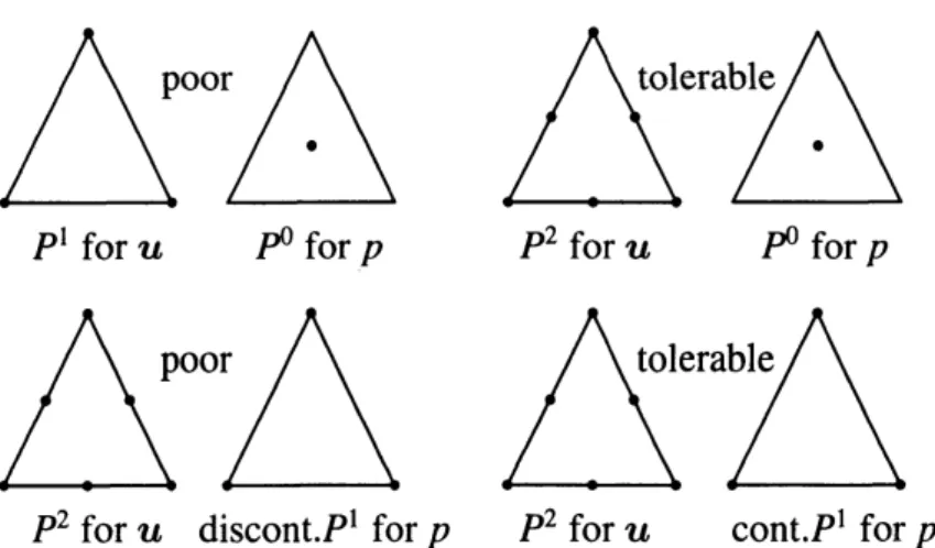
choose$k_{p}$ tobe smaller than$k$, but thevalidity of such approximations depends strongly

on

the arrangement of nodes

as

well. For example, the $P^{1}-P^{0}$ triangle _(continuous $P^{1}$

for $u_{h}$

and discontinuous $P^{0}$ for

$p_{h}$) is not appropriate, while $P^{2}-P^{0}$ triangle works. Moreover, $P^{2}$

-cont.$P^{1}$ works,

while$P^{2}$

-discont.$P^{1}$ behavesbadly. SeeFig.2for

a

fewtypical

$P^{1}$ for

$u$ $P^{0}$ for

$p$ $P^{2}$ for$u$ $\mu$ for$p$

$P^{2}$

for$u$

discont.Pl

for$p$ $P^{2}$

for $u$

cont.Pl

for$p$

Figure2: Some combinations of$u$ and$p$for triangles

To analyze $[MF]_{h}$, it is essentialto show the followingdiscrete inf-sup condition: There

existsa constant$K>0$_suchthat, $\forall h>0,$

$inf\sup \underline{(divv_{h},q_{h})_{\Omega}}\geq K$

_.

(16)

$v_{h}\in(V_{0}^{h})^{N}\backslash \{0I_{q_{h}\in W_{0}^{h}\backslash \{0\}}\Vert v_{h}\Vert_{H_{0}^{1}(\Omega)^{N}}\cdot\Vert q_{h}\Vert_{\Omega}$

A typical approach to show the above is to construct

a

Fortin operator $\Pi_{h}^{F}$

:

$H_{0}^{1}(\Omega)^{N}arrow$ $(V_{0}^{h})^{N};\forall v\in H_{0}^{1}(\Omega)^{N},$

$||\Pi_{h}^{F}v||_{H^{1}(\Omega)^{N}}\leq C||v||_{H^{1}(\Omega)^{N}}, (div(\Pi_{h}^{F}v-v), q_{h})_{\Omega}=0;\forall q_{h}\in W^{h}$

.

(17)

A number of trials have been madeto find such $\Pi_{h}^{F}[6]$,though it isnot

so easy a

task.

6

Hybrid

discontinuous Galerkin FEM

We

can

also

use

discontinuous,

more

flexible

approximate

displacementsbased

on

thehybrid

discontinuous GalerkinFEM (HDGFEM). In thiscase,

we use

discontinuous element-wise

polynomial functions for $u$ (and p) and also the so-called fluxes$\hat{u}$ (inter-element

displace-ments)

_as

_{independent unknown functions}[8, 13]. Onthe otherhand,intheoriginal

discon-tinuous Galerkin (DG)FEM, fluxes

are

calculated from $v[2].$

We willconsider only the 2-D

cases

$(N=2)$,and

assume

that$\Omega$is aboundedpolygonal

domain withboundary $\partial\Omega$

.

Moreover,

we

will also

use

(possiblyfractional) Sobolev

spaces

$W^{s,p}(\Omega)$and $W_{0}^{s,p}(\Omega)$for $1\leq p\leq\infty,$ $s\geq 0$,whose

norm

andstandardsemi-norm

are

denoted

by $||\cdot||_{s,p,\Omega}$ and $|\cdot|_{s,p,\Omega}$,respectively. Moreover, $s$is omitted when $s=0$

.

When$p=2$ , they

are

alsowrittenby $H^{s}(\Omega)$and$H_{0}^{s}(\Omega)$,and the thesubscript$p$in the

norms

andsemi-norms is

omitted. We willessentially dealwith theHilbertian

cases

$(p=2)$ , but sometimes consider

more

general

cases.

To take theconsistency between the

case

$p=2$ andothers $(p\neq 2)$ for

(semi-)norms,

we

for example define $\Vert\nabla u||_{p,\Omega}$ by $|| \nabla u||_{p,\Omega}^{p}=\sum_{i=1}^{2}||\partial u\int\partial x_{i}\Vert_{p,\Omega}^{p}$ for $1\leq p<\infty$

6.1

Triangulations

by

finite elements

We will

use

$\{\mathcal{T}^{h}\}_{h>0}$

as

a

“regular family of triangulations of $\Omega$

.

The precise meaning of

“regular” is omitted here (see e.g.[3, 12 roughly speaking, it

means

that the shapes of

finite elements (see below)

are

not too much distorted and their sizes

are

comparable. In

the presentsettings, each triangulation$\mathcal{T}^{h}$

consists offinite number ofbounded$m$-polygonal

finite elements $K’ s$_, where $m$ is

an

integersuch that $3\leq m\leq M$ ($M\geq 3$ is

a

constant) and

can

differ with$K$

.

Theboundary of$K\in \mathcal{T}^{h}$ is

a

closed simple polygonal lineand denotedby

$\partial K$

.

Notice here that each finite

element (orelement, in short) $K$ is not necessarily

convex

and vertexes with the flat angle

are

allowed. The number$h_{K}$ stands for the diameter of$K,$

and themesh parameter$h$ofthe triangulation is defined by$h= \max_{K\in \mathcal{T}^{h}}h_{K}$

.

An(open) edge

of$K$is designated by$e$, andits lengthby $|e|$

.

Wedefine$S^{K}$ and$S^{h}$

as

the sets of alledges in $K\in \mathcal{T}^{h}$

and $\mathcal{T}^{h}$

, respectively. Moreover, $\Gamma^{h}=\bigcup_{e\in S^{h}}\overline{e}$ is called the skeleton of$\mathcal{T}^{h}$

.

Almost

everywhere

on

$\partial\Omega$

and$\partial K$

,

we can

define theunitoutwardnormal vector$n=\{n_{1},n_{2}\}.$

As duality pairings

or

innerproducts relatedtoeach element $K\in \mathcal{T}^{h}$,

we

will

use:

$)_{K}$

:

dualitypairingbetween$L^{p}(K)^{\ell}$and_{$L^{q}(K)^{\ell}(\ell=1, 2, 1/p+1/q=1)$}

as

theextension

of theinnerproduct of$L^{2}(K)^{\ell}$,i.e., forexamplefor$\ell=1,$ $(u, v)_{K}= \int_{K}$uvdx $(u\in L^{p}(K)$,

$v\in L^{q}(K))$,

$]_{\partial K},$ $]_{e}$,resp.)

:

dualitypairingbetween$L^{p}(\partial K)^{\ell}$($L^{p}(e)^{\ell}$foredge$e\in S^{K}$_{,resp.) and}

$L^{q}(\partial K)^{\ell}$ ($L^{q}(e)^{f}$,resp.) $(\ell=1,2,1/p+1/q=1)$

as

theextensionof theinnerproduct

of$L^{2}(\partial K)^{\ell}$ ($L^{2}(e)^{\ell}$,resp.).

Moreover,$L^{p}$ type

norms

related to$K$

are

denotedby: $||\cdot||_{p,K}$

:

norm

of$L^{p}(K)^{\ell}(\ell=1,2)$,

$|\cdot|_{p,\partial K}$ $(|\cdot|_{p,e},$

resp.

$)$

: norm

of$L^{p}(\partial K)^{f}$($L^{p}(e)^{\ell}$,resp.) _$(\ell=1,2)$

.

We will oftenomitthe suffix$p$of

norms

andinner productsfor$p=2.$

Figure3: $K,$ $K’,$$e,$ $u$and $\hat{u}$

6.2

Function

spaces

dependent

on

$\mathcal{T}^{h}$

For

our

purposes,

itis essentialto

use

the broken(orpiecewise)Sobolevspace$\Pi_{K\in \mathcal{T}^{h}}W^{s,p}(K)$

$(1\leq p\leq\infty, s>0)$

on

$\mathcal{T}^{h}$

,which is identified with

Iistobe notedthat,for$v\in W^{1/p+\gamma,p}(\mathcal{T}^{h})(\gamma>0)$,thetrace

v

$|_{\partial K}$of$v|_{K}(K\in \mathcal{T}^{h})$to$\partial K$belongs

to$L^{p}(\partial K)$, and

may

be double-valued

on an

inter-element edge$e$ sharedby two elements $K$

and$K’:(v|_{K})|_{e}$ may notcoincide with $(v|_{K’})|_{e}.$

In HDG FEM,

we

also

use

$U$ functions

on

the skeleton $\Gamma^{h}$

, which

are

called numerical

fluxes.

It is important that each $\hat{v}\in L^{p}(\Gamma^{h})$ is single-valued

on

$\Gamma^{h}$

, unlike the traces of

$v\in Hz^{\iota_{+\gamma}}(\mathcal{T}^{h})(\gamma>0)$ to $\Gamma^{h}$

.

To account for the homogeneous Dirichletcondition,

we

also

introduce thefollowing

space on

$\Gamma^{h}$

:

$L_{D}^{p}(\Gamma^{h})=\{\hat{v}\in L^{p}(\Gamma^{h});\hat{v}=0 on \partial\Omega\}$ (19)

In the HDG methods, the numerical flux $\hat{v}$ is independent of the function

$v$ taken for

example from $W^{1,p}(\mathcal{T}^{h})$

.

On the otherhand, in the original DGmethods, the flux is rather

a

subsidiaryfunction, and, when

necessary,

it is derived from $v$

.

We will only consider the

mosttypicalderivation of$\hat{v}$

:

if$e\in S^{h}$is sharedby two elements$K$and$K’,$ $\hat{v}|e$is given by

$\hat{v}|_{e}=\frac{1}{2}((v|_{K})|_{e}+(v|_{K’})|_{e})$ _, (20)

while if$e\subset\partial\Omega,$ $\hat{v}|_{e}$ istaken

as

either$0$

or

$v|_{e}$ in accordance with the homogeneous Dirichlet

condition is considered

or

not[2]. The

spaces

thus induced

are

also denotedby $0^{h}$ and $O_{D}^{h}.$

Over $W^{1,p}(\mathcal{T}^{h})\cross L^{p}(\Gamma^{h})$, define $W^{1,p}$-type semi-norm and

norm

for $\{v, \hat{v}\}\in W^{1,p}(\mathcal{T}^{h})\cross$ $L^{p}(\Gamma^{h})$respectively by

$| \{v, \hat{v}\}|_{1,p,h}^{p}=||\nabla_{h}v||_{p,\Omega}^{p}+\sum_{K\in \mathcal{T}^{h}}\sum_{e\in S^{K}}\frac{1}{|e|^{p-1}}|v-\hat{v}|_{p,e}^{p},$ $||\{v, \hat{v}\}||_{1,p,h}^{p}=\{v, \hat{v}\}|_{1,p,h}^{p}+||v||_{p,\Omega}^{p}$, (21)

where $\nabla_{h}v\in W^{1,p}(\mathcal{T}^{h})^{2}$ is characterized by $(\nabla_{h}v)|K=\nabla(v|K)\in L^{p}(K)(\forall K\in \mathcal{T}^{h})$

.

The

last term in $|\{v, \hat{v}\}|_{1,p,h}^{p}$ is used

as a

measure

of discontinuity of $v$ along the inter-element

boundaries together with thediscrepancy of$v$ fromthe Dirichlet condition

on

$\partial\Omega$

.

A similar

termwith

some

coefficients will be used later

as

the interior penaltyterm.

6.3

Finite

element

spaces

for

HDG

FEM

For$k\in N$_, let

us prepare

the following finite dimensional

spaces:

$U^{h}=\Pi_{K\in \mathcal{T}^{h}}P^{k}(K)\subset W^{2,\infty}(\mathcal{T}^{h})$, (22) $\hat{U}^{h}=\Pi_{e\in\epsilon}hP^{k}(e) (or \Pi_{e\in\epsilon^{h}}P^{k}(e)\cap C(\Gamma^{h}))\subset L^{\infty}(\Gamma^{h}) , \hat{[Ucirc]}_{D}^{h}=\hat{U}^{h}\cap L_{D}^{\infty}(\Gamma^{h})$, (23)

where $P^{k}(K)$ and $P^{k}(e)$

are

polynomial

spaces on

$K$ and $e$ of degree $\leq k$, respectively. For

$\hat{U}^{h}$

, the

case

$0_{h}\subset C(\Gamma^{h})$ (space of continuous numericalfluxes) is in

a sense

natural

as

the

spaceoftracesfrom $W^{1,p}(\Omega)$to$\Gamma^{h}$

atleast when$p\geq 2$

.

However, $0^{h}$ whoseelements

can

be

discontinuousat vertexesis also used and

may

besometimes superiortothecontinuous

one.

Now typical examples offinite element

spaces

used forapproximating scalar functions

in $W^{1,p}(\Omega)$ and $W_{0}^{1,p}(\Omega)$ are, respectively,

$V^{h}=U^{h}\cross 0^{h}\subset W^{2,\infty}(\mathcal{T}^{h})\cross L^{\infty}(\Gamma^{h})$, $V_{D}^{h}=U^{h}\cross O_{D}^{h}\subset W^{2,\infty}(\mathcal{T}^{h})\cross L_{D}^{\infty}(\Gamma^{h})$

.

(24)

As

was

already noted, the approximate flux $\hat{v}$

is derived from $v\in U^{h}$ _{in the original DG}

6.4

Lifting

operators

InDGFEM,variousfunctions

on

edges and$\Gamma^{h}$

appear

andplay essential roles. To associate

them with

some

functions

on

$K’ s$_,

we

often

use

the so-calledliftingoperators,whose typical

examples

are

introduced below.

For$K\in \mathcal{T}^{h}$ and the former$k\in \mathbb{N}$,let

us

introduce $Q^{K}\subset L^{\infty}(K)$

as

$Q^{K}=P^{k}(K)$

or

$P^{k-1}(K)$. (25)

Then thelocal liftingoperators$R_{Ki}(i=1,2)$

:

$g\in L^{p}(\partial K)\mapsto\xi_{j}\in Q^{K}$

are

defined by

$(\xi_{i}, \eta)_{K}=[g, \eta n_{i}]_{\partial K}(\forall\eta\in Q^{K})$, (26)

where $n=\{n_{1}, n_{2}\}$ isthe outwardunitnormal

on

$\partial K$

.

Clearly,$\xi_{i}=R_{Ki}g$ exists uniquely for

each $i(=1,2)$

.

The global liftingoperators$R_{hi}(i=1,2)$

are

given, roughly speaking,by assemblingthe

local

ones

element by element. Moreprecisely, with $Q^{h}:=\Pi_{K\in \mathcal{T}^{h}}Q^{K}\subset L^{\infty}(\Omega)$,$R_{hi}$ foreach $i\in\{1$,2$\}$ is defined by

$R_{hi}:\tilde{g}=\{g_{\partial K}\}_{K\in \mathcal{T}^{h}}\in\Pi_{K\in \mathcal{T}^{h}}L^{p}(\partial K)\mapsto\{R_{Ki}g_{\partial K}\}_{K\in \mathcal{T}^{h}}\in Q^{h}$ (27)

Theliftingoperators of the present form

are

usedtoapproximatesuch

a

boundary integral

$[g, n_{i}\partial u/\partial x_{i}]_{\partial K}(i\in\{1,2\})$ by

an

integral

over

$K$

.

If $u$is approximated by

a

$P^{k}$ function $u_{h}$ in

$K,$ $\partial u_{h}/\partial x_{j}|_{K}$is a$P^{k-1}$ function, sothat $(\xi_{i}, \eta)=[g, n_{i}\eta]_{\partial K}(\xi_{i}=R_{Ki}g, \eta\in P^{k} or P^{k-1})$gives

$(R_{Ki}g, \partial u_{h}/\partial x_{i})_{K}=[g, n_{j}\partial u_{h}/\partial x_{j}]_{\partial K}(i=1,2)$

.

(28)

Moreover, when $k=1$ and $Q^{K}=P^{0}(K)$, any $P^{1}$ function

$v_{h}$ in $K$ satisfies $(\partial v_{h}/\partial x_{j}, \eta)_{K}=$

$[v_{h}, n_{i}\eta]_{\partial K}$by the Gaussformula,

so

thatthe relation$(R_{Ki}v_{h}, \eta)_{K}=[v_{h}, n_{i}\eta]_{\partial K}$

recovers

$\partial v_{h}/\partial x_{i},$

i.e.,

$R_{Ki}(v_{h}|_{\partial K})=\partial v_{h}/\partial x_{i}(k=1, Q^{K}=P^{0}(K))$

.

(29)

It is to be noted that the present flux $\hat{v}\in L^{p}(\Gamma^{h})$ is single-valued

on

$e\in S^{h}$, and is

considered an element of$\Pi_{K\in \mathcal{T}^{h}}L^{p}(\partial K)$

.

On the other hand, the trace of$v\in W^{1,p}(\mathcal{T}^{h})$ to$e$

can

bedouble-valued. To

use

$R_{hi}$ to such$v$,let

us

introduce theoperator:

$S_{h}:v\in W^{1,p}(\mathcal{T}^{h})\mapsto\{v|_{\partial K}\}_{K\in \mathcal{T}^{h}}\in\Pi_{K\in \mathcal{T}^{h}}L^{p}(\partial K)$

.

(30)

By using $S_{h}$,

we

can

apply $R_{hi}(i=1,2)$ to an element such

as

$S_{h}v-\hat{v}$, which belongs to

$\Pi_{K\in \mathcal{T}^{h}}L^{p}(\partial K)$ (alsoto$\Pi_{K\in \mathcal{T}^{h}}L^{\infty}(\partial K)$in thepresent choice of$V^{h}$ in (24)and $Q^{K}$ in (25)), the

domain of definition of$R_{hi}.$

7

Some theoretical

results

for

DG

FEM

In thissection,

we

will present

some

theoretical results for DG FEM. In the former parts,the

functions

are

essentially scalar ones,whilevectorfunctions willbe also considered later. We

will essentially considerthe

cases

for $1<p<\infty$, although

some

results may also hold for

7.1

Regularization

of

discontinuous

functions

7.1.1 Assumptions

on

thefamilyof triangulations

To derive various theoretical results for HDGFEM,

we

must impose

some

assumptions

on

$\{\mathcal{T}^{h}\}_{h>0}$

.

We havealready stated that thenumber of elements in $\mathcal{T}^{h}$

is finite, and the number

of edges of each bounded polygonal finite element $K\in \mathcal{T}^{h}$ is bounded from above by

a

positive integer$M$independently of$h$and _$K[3$, 12$].$

Weadd

a

geometricalassumptioncalled thechunkiness condition duetoDeny-Lions and

Brenner-Scott[3]. Thatis,forany $h>0$ and$K\in \mathcal{T}^{h}$,there exists

an open

disk_{$D_{K}$} of radius

$\rho_{K}>0$ inscribedto$K$such that$K$is star-shapedwith respectto any points in$D_{K}$ and $\rho_{K}/h_{k}\geq\eta$, (31)

where$\eta$ is

a

positiveconstant

common

toallthe elements in the family

$\{\mathcal{T}^{h}\}_{h>0}.$

For the above$D_{K}$ of$K$_, let

us

denote its center by $C^{K}$

.

Foreach edge $e\in S^{K}$_, define by

$\theta_{e}$ theinterior angle at $C^{K}$ of the trianglecomposedof$C^{K}$ and $e$

.

Then,

we

furtherassume,

for

a

positiveconstant $\theta_{0},$

$\theta_{e}\geq\theta_{0}(\forall h>0, \forall K\in \mathcal{T}^{h}, \forall e\in S^{K})$

.

₍₃₂₎

From this assumption,

we can

conclude the finiteness of number of edges of$K$but alsothat

the edgelength$|e|$ is bounded from below by

a

constanttimes$h_{K}.$

7.1.2 Evaluation of liftingoperatorsby interiorpenaltyterms

Foranalyzing the DG methodusinglifting operators,

we

must evaluatethem intermsof the

interior penalty terms. To do this,

we can use

the duality operators from $L^{p}(K)$ to $L^{q}(K)$

$(1<p<\infty, q=p/(p-1))[5$, 7$]$,and then

we

have thefollowing results.

Lemma 1 For$h>0,$ $K\in \mathcal{T}^{h}$ and_$i=1$,2, it holds

for

$g\in L^{p}(\partial K)$that

$||R_{Ki}g||_{p,K} \leq C_{p}[\sum_{e\in\epsilon^{\kappa}}\frac{1}{|e|p-1}|g|_{p,e}^{p}]^{\iota/p}$ (33)

where $C_{p}>0$is dependenton$p$but independent

of

$g,$ $h,$ $K$and$i.$

7.1.3 Vertex averaging operator

Letus first considerthe vertex averaging operator forthe numerical fluxes. Essentially the

same

idea

was

introduced by Brenner[4] for the original DG FEM, and has been used in

many

literatures. In the HDG FEM, such averaging

process

is

unnecessary

if $\hat{[Ucirc]}^{h}\subset C(\Gamma^{h})$,

while itis effective in general HDG and original DG FEM where numerical fluxes

may

be

discontinuousatvertexes.

Let

us

consider the numerical flux $\hat{v}_{h}\in 0^{h}$, where $O^{h}$ is either independent of$U^{h}$ in the

presentHDG FEM

or

derived from $U^{h}$ in the original (non-hybrid) DG FEM. In

any

cases,

they

are

piecewisepolynomials

on

$\Gamma^{h}$

.

Then foreachvertex$p\in\Gamma^{h}$,define$(\ovalbox{\tt\small REJECT}_{h}v_{h})(p)$ by

where$T_{p}$is the setof edges thathave$p$

as an

endpoint, i.e., $T_{p}=\{e\in S^{h};p\in\overline{e}\}$, and $|Y_{p}|$

is the numberof edges in$T_{p}$,which is finite andboundedfromabove by

a

positiveconstant

under appropriate regularity conditions

on

$\{\mathcal{T}^{h}\}_{h>0}$

.

For

a

continuous flux, it clearly holds

that$(\ovalbox{\tt\small REJECT}_{h}\hat{v}_{h})(p)=\hat{v}_{h}(p)$ foranyvertex$p\in\Gamma^{h}.$

As Lemma2.1 of [4],thefollowinglemmaholds.

Lemma 2 There exists apositive constant common to $\{\mathcal{T}^{h}\}_{h>0}$ such that,

for

any $\{v_{h}, \hat{v}_{h}\}\in$ $U^{h}\cross O^{h}$_, any_vertex$p\in\Gamma^{h}$ and any_{$e\in Y_{p},$}

$| \lim_{q\in earrow p}\hat{v}_{h}(q)-(\ovalbox{\tt\small REJECT}_{h}\hat{v}_{h})(p)|\leq C\sum_{e\in T_{p}}\sum_{K\in \mathcal{T}^{e}}|\lim_{q\in Karrow p}v_{h}(q)-\lim_{q\in earrow p}\hat{v}_{h}(q^{*})|$, (35)

where$\mathcal{T}^{e}$ is theset

of

elements that have$e\in S^{h}$ as their edge, i.e., $\mathcal{T}^{e}=\{K\in \mathcal{T}^{h};e\subset\partial K\}.$

7.1.4

Discreteinverse tracetheorems

We will introduce

a

$2D$discreteinverse_trace,

or

trace lifting, operator, whichmaps

continu-ous

numericalfluxesin $\hat{U}^{h}\subset C(\partial K)$to functions in _$W^{1,p}(K)$

.

Let

us

state the trivial ID discrete trace theorem, which is shown by using the linear

interpolationfunctions withtwoend-points used

as

the samplingpoints.

Lemma3 Let$I=[0, L]$

_for

$L>0$, and$a,$ $b\in \mathbb{R}$

.

Then thereexists

a

unique linear

polyno-mial

_function

$\hat{v}\in C(I)$such that$\hat{v}(O)=a,$ $\hat{v}(L)=b$, and

$| \hat{v}|_{pJ}\leq(\frac{2^{p-1}L}{p+1})^{1/p}(|a|^{p}+|b|^{p})^{1/p}(1\leq p<\infty)$_, $| \hat{v}|_{\infty J}\leq\max\{|a|, |b|\}(p=\infty)$_{, (36)}

$where|\cdot|_{pJ}$ denotes the

norm over

$L^{p}(I)$

.

The following lemma is

a

discrete analog ofthe

inverse

trace theorem, but in the

orig-inal inverse trace theorem, functions

on

$\partial K$

are

taken from $W^{1-1/p,p}(\partial K)$, the trace

space

of $W^{1,p}(K)$

.

The assumption $\hat{v}\in C(\partial K)$ below is essential for $\hat{v}$ to

belong to $W^{1-1/p,p}(\partial K)$

especiallywhen$p\geq 2.$

Lemma4 Let$h>0,$ $K\in \mathcal{T}^{h},$ $k\in \mathbb{N},$ $1<p<\infty$ and$\hat{v}\in\Pi_{e\in S^{K}}P^{k}(e)\cap C(\partial K)$

.

Then there

existsa

_function

$v\in W^{1,p}(K)$ such that$v|_{\partial K}=\hat{v}$and

$|v|_{1,p,K}+h_{K}^{-1}||v||_{p,K}\leq C_{p}h_{K}^{1/p-1}|\hat{v}|_{p,\partial K}$_, (37)

where $h_{K}$ is the diameter

of

$K$_, and$C_{p}$ is

a

positive constantdepending onlyon $p$under the

presentregularity conditions

on

$\{\mathcal{T}^{h}\}_{h>0}.$

7.1.5 Regularization of discontinuous functionsin $U^{h}$

By Lemmas 2 and 3,

we can

construct a continuous flux from the original one, and the

difference between themis bounded by the interior penalty. Then using Lemma4 and the

above continuous flux,

we

obtain

a

$W^{1,p}(\Omega)$ function, whose difference from the original

$W^{1,p}(\mathcal{T}^{h})$ functionis againevaluated by the interior penaltyterm.

Thepresentprocess is essentiallythe

same

as

the

use

of thereconstruction presented by

Lemma5 Let

us

consider $\{\mathcal{T}^{h}\}_{h>0}$and $\{v_{h}, \hat{v}_{h}\}\in U^{h}\cross\hat{U}^{h}$ associatedwith

a

$\mathcal{T}^{h}$

.

Then there

exists a

_function

$v^{h}\in W^{1,p}(\Omega)$suchthat

$|| \nabla v^{h}-\nabla_{h}v_{h}||_{p,\Omega}+h^{-1}||v^{h}-v_{h}\Vert_{p,\Omega}\leq C_{p}(\sum_{K\in \mathcal{T}^{h}}\sum_{e\in S^{K}}\frac{1}{|e|^{p-1}}|v_{h}-\hat{v}_{h}|_{p,e}^{p})^{1/p}(h=\max_{K\in \mathcal{T}^{h}}h_{K})$_, (38)

where $C_{p}>0$depends only

on

$p$under thepresentregularity conditions

on

$\{\mathcal{T}^{h}\}_{h>0}.$

Using the above results,

_we

can

derive the discrete versions of the Poincar\’e-Friedrichs

inequalities, the Rellich-Kondrashov theorem, the Kom inequalities etc., which

are

all

im-portant tools in numericalfunctional analysis.

7.2

$2D$

discrete

Rellich-Kondrashov theorem

Since $W^{1,p}(\mathcal{T}^{h})$ ismuch wider than $W^{1,p}(\Omega)$_,

we

must

prove

variousdiscrete versionsof

the-orems

relatedto the Sobolev spaces such

as

the Rellich-Kondrashov compactness theorem.

The author derived the Rellich-type theorem $(p=2)[12$, 14$]$, and here give its extension

to

more

generalcases, i.e., discrete Rellich-Kondrashovtheorem by using the discretetrace

lifting theorem and Lemma 1. Itis to be noted that the strong

convergence

in $L^{p}(\Omega)$ below

is generalizedto

more

generalvalues otherthan $p$depending

on

the valueof$p$,although

we

omitthe detail here.

Theorem 1 Under the regularity conditions[3, 12]

_of

$\{\mathcal{T}^{h}\}_{h>0}$, consider anyfamily$\{\{u_{h}, \hat{u}_{h}\}\in$

$V^{h}\}_{h>0}$ $(\{\{u_{h},\hat{u}_{h}\}\in V_{D}^{h}\}_{h>0},$ respectively)associatedto $\{\mathcal{T}^{h}\}_{h>0}$such

$that|\{u_{h}, \hat{u}_{h}\}|_{1,p,h}^{p}+||u_{h}||_{p,\Omega}^{p}\leq$

$1$

.

Thenthereexist$u_{0}\in W^{1,p}(\Omega)$₍$u_{0}\in W_{0}^{1,p}(\Omega)$, respectively)and

a

sub-family, again denoted

by $\{\{u_{h}, \hat{u}_{h}\}\}_{h>0}$, such that

as

$h\downarrow 0$

$u_{h}arrow u_{0}$ stronglyin$L^{p}(\Omega)$, $u_{h}|_{\partial\Omega}arrow 0$ stronglyin$L^{p}(\partial\Omega)$

if

$\{u_{h}, \hat{u}_{h}\}\in V_{D}^{h}$, (39) $\nabla_{h}u_{h}+R_{h}(\hat{u}_{h}-S_{h}u_{h})arrow\nabla u_{0}$ weaklyin $L^{p}(\Omega)^{2}$ with _{$R_{h}=\{R_{h1},R_{h2}\}$}

.

(40)

7.3

Approximate derivatives

in DG

FEM

In view of the former theorem, the lifting term in $\nabla_{h}u_{h}+R_{h}(\hat{u}_{h}-S_{h}u_{h})$ is essential, and

is related to thejumps

on

the inter-element boundaries:

even

when this term is not used,

something

more

orless alike is necessary as an alternative.

As

an

approximation ofusualderivative$\partial v/\partial x_{j}(i=1,2)$ for $v\in H^{1}(\Omega)$_,

we

will

use

the

following$\partial_{h,i}\{v, \hat{v}\}$ for $\{v, \hat{v}\}\in H^{1}(\mathcal{T}^{h})\cross L^{2}(\Gamma^{h})$based

on

thelifting operator$R_{Ki}$

:

$(\partial_{h,i}\{v,\hat{v}\})|_{K}=\partial(v|_{K})/\partial x_{i}+R_{Ki}(\hat{v}|_{\partial K}-(v|_{K})|_{\partial K})(i=1,2)$

.

Inthe present HDGFEM,

we

will

use

suchapproximatederivatives instead of the usual

ones

8

$2D$

plain

strain

problem

8.1

Preparations for

HDG FEM

As the $2D$ displacementin

our

approach,

we

will

use

$\tilde{u}=\{u, \hat{u}\}\in H^{1}(\mathcal{T}^{h})^{2}\cross L^{2}(\Gamma^{h})^{2}$ with $u=\{u_{1}, u_{2}\}$ and \^u $=$ $\{\hat{u}_{1}, \hat{u}_{2}\}$

.

Then,

as

approximate derivatives tobe used for approximate

strains,

we

adopt $\partial_{h,i}\{v, \hat{v}\}(i=1,2)$ for $\{v, \hat{v}\}\in H^{1}(\mathcal{T}^{h})^{2}\cross L^{2}(\Gamma^{h})^{2}$

as

proposed in the

preceding subsection. Thusthe approximatestrains $e_{h,ij}(\tilde{u})(1\leq i, j\leq 2)$ and divergence

are

expressed by

$e_{h,ij}( \tilde{u})|_{K}=\frac{1}{2}(\partial_{h,j}\{u_{j},\hat{u}_{i}\}+\partial_{h,i}\{u_{j},\hat{u}_{j}\}) , div_{h}\tilde{u}=\sum_{i=1}^{2}e_{h,ii}(\tilde{u})$, (41)

whilethe stresses

are

derived from the strainsby thegeneralized Hooke law:

$s_{h,ij}(\tilde{u})=\lambda\delta_{ij}div_{h}\tilde{u}+2\mu e_{h,ij}(\tilde{u})$ $(1\leq i, j\leq 2)$ with $p_{h}(\tilde{u})=-\lambda_{B}div_{h}\tilde{u}$

.

(42)

We will essentially

use

thefollowing bilinear form for$\tilde{u},$ $\tilde{v}\in H^{\frac{3}{2}+\gamma}(\mathcal{T}^{h})^{2}\cross L^{2}(\Gamma^{h})^{2}$ with

$\gamma>0$

:

$a_{h,\sigma}( \tilde{u},\tilde{v})=\sum_{i,j=1}^{2}\{[\sum_{K\in \mathcal{T}^{h}}(e_{ij}(u), e_{ij}(v))_{K}+[\hat{u}_{i}-u_{i}, e_{ij}(v)n_{j}]_{\partial K}+[\hat{v}_{j}-v_{i}, e_{ij}(u)n_{j}]_{\partial K}]$

$+ \frac{1}{4}(R_{hj}(\hat{u}_{i}-S_{h}u_{j})+R_{hi}(\hat{u}_{j}-S_{h}u_{j}),R_{hj}(\hat{v}_{i}-S_{h}v_{i})+R_{hi}(\hat{v}_{j}-S_{h}v_{j}))_{\Omega}\}$

$+ \sigma\sum_{K\in \mathcal{T}^{h}}\sum_{e\in S^{K}}\sum_{i=1}^{2}\frac{1}{|e|}[u_{i}-\hat{u}_{i}, v_{i}-\hat{v}_{i}]_{e}$, (43)

$d_{h}( \tilde{u},\tilde{v})=\sum_{K\in \mathcal{T}^{h}}[(divu, divv)_{K}+\sum_{i=1}^{2}([\hat{u}_{j}-u_{i}, (divv)n_{i}]_{\partial K}+[\hat{v}_{i}-v_{i},(divu)n_{i}]_{\partial K})]$

$+ \sum_{i,j=1}^{2}(R_{hi}(\hat{u}_{i}-S_{h}u_{i}),R_{hi}(\hat{v}_{i}-S_{h}v_{i}))_{\Omega}$, (44)

where the assumption$\gamma>0$is required to

assure

theexistence of

some

traces, the lastterm

in $a_{h,\sigma}(\cdot, \cdot)$ is the interior penalty one, and $\sigma\geq 0$ is the penalty parameter which is usually

chosen to be 0(1). Moreover, the terms involving $R_{hi}$’s

are

omitted in

some

primitive DG

andHDGFEM[13], but then$\sigma$ mustbe chosen sufficiently largeto

assure

the positivity of

the above bilinear forms.

8.2

Basic

HDG FEM

_in

$\tilde{u}$

only

Wewill

use

the$P^{k}$

finiteelement

spaces

(22) and(23)for$\tilde{u}=\{u,$$u$

Then

a

typical FE

formulation

is, for

a

given

$f\in L^{2}(\Omega)^{2}$,tofind $\tilde{u}_{h}=\{u_{h},\hat{u}_{h}\}\in\tilde{V}_{D}^{h}s.t.$

$2\mu a_{h,\sigma}(\tilde{u}_{h},\tilde{v}_{h})+\lambda d_{h}(\tilde{u}_{h},\tilde{v}_{h})_{\Omega}=(f, v_{h})_{\Omega}(\forall\tilde{v}_{h}=\{v_{h},\hat{v}_{h}\}\in\tilde{V}_{D}^{h})$, (46)

where

we can

rewritethe approximatebilinear forms by

$a_{h,\sigma}( \tilde{u}_{h},\tilde{v}_{h})=\sum_{i.j=1}^{2}(e_{h,ij}(\tilde{u}_{h}), e_{h,ij}(\tilde{v}_{h}))_{\Omega}+\sigma\sum_{K\in \mathcal{T}^{h_{e}}}\sum_{\epsilon^{K}}\sum_{i=1}^{2}\frac{1}{|e|}[u_{i}-\hat{u}_{i}, v_{i}-\hat{v}_{i}]_{e}$, (47)

$d_{h}(\tilde{u}_{h},\tilde{v}_{h})=(div_{h}\tilde{u}_{h}, div_{h}\tilde{v}_{h})_{\Omega}$

.

(48)

The unique solvability of the above problem is straightforward provided that the Kom-typeinequalities(seethesubsequentsubsection)

_are

_{establishedtogetherwith}

_some

standard requirements in DGFEM[2]. However,

its

behaviors

as

$\lambdaarrow\infty$isnotclear at present.

More-over, under appropriate regularity conditions

on

the exact solution,

we can

derive various

error

estimates

as

routineworks.

8.3

A discrete

$2D$

Korn’s inequality

Forthe validity of the present approximation, it is again essential to show discrete versions

of Kom’s inequalities. We have shown, for $\mu/\mu$ approximation $(P^{k}(K)$ for $u_{i},$ $P^{k}(e)$ for

$\hat{u}_{j})[15]$ for$p=2$,which

can

begeneralizedfor $1<p<\infty$

:

Lemma6 There existsa constant$C_{p.\Omega}>0$ (dependenton $p(1<p<\infty)$ and$\Omega$), _$s.t.$,

for

any small$h(0<h\leq h)$andany$\tilde{v}_{h}=\{v_{h}, \theta_{h}\}=\{\{v_{h1}, v_{h2}\}, \{\hat{v}_{h1}, \hat{v}_{h2}\}\}\in\tilde{V}^{h},$

$\sum_{K\in \mathcal{T}^{h}}\sum_{i,j=1}^{2}\Vert\frac{1}{2}(\partial_{j}v_{hi}+\partial_{i}v_{hj})\Vert_{p,K}^{p}+\sum_{i=1}^{2}\sum_{\kappa er^{h}}\sum_{e\in8^{K}}\frac{1}{|e|^{p-1}}|v_{hi}-\hat{v}_{hi}|_{p,e}^{p}+||v_{h}||_{p,\Omega}^{p}\geq C_{p}||\tilde{v}_{h}||_{1,p,h}^{p}(49)$

where the $tenn||v||_{p,\Omega}^{p}$

can

be

omittedfor

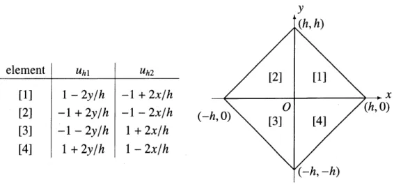
$\tilde{v}\in\tilde{V}_{D}^{h}.$

Remark2 For the non-conforming$P^{1}$ triangle

of

Crouzeix-Raviart, $Kom$_-type inequalities

do not hold.

_If

the mesh contains the patch in Fig.4 and $u_{h}=\{u_{h1}, u_{h2}\}$ is

zero

outside

$it$_, this non-confonning displacement_cannot satisfy Korn-type inequalities_[11], although it

certainlydoes

_for

the completely incompressible

case

where the divergence-free condition is

imposedelement-wise, see [1]. _{Notice that this triangularfinite elementmethod is themost}

elementaryDGFEM.

8.4

Mixed

type HDG FEM

in

$\tilde{u}$

and

$p$

Itis alsopossibleto add$p$

as

an independent unknown function, andsuch

an

approach is

an

mixed type HDG FEM. We introduce

a

space

$W^{h}$for

$p$such

as

$\Pi_{K\not\in\Gamma^{h}}P^{k_{p}}(K)$with$0\leq k_{p}\leq k,$

and also

use

$W_{0}^{h}=W^{h}\cap L_{0}^{2}(\Omega)$

.

Then

a

mixed HDG FEMisto find$\{\tilde{u}_{h},p_{h}\}\in\tilde{V}_{D}^{h}\cross W^{h}s.t.$

Figure 4: Exampleofpatchoftriangularelements

Remark3 Since $\hat{u}_{h}\in O_{D}^{h}$,

we can

show that $(div_{h}\tilde{u}_{h}, 1)_{\Omega}=0$by the Green

formula.

Thus

the present $p_{h}$ necessarily belongs to $W_{0}^{h}$

. If

$div_{h}\tilde{V}_{D}^{h}\subset W^{h}$ and $\lambda$ is finite, we have $p_{h}=$ $-\lambda_{B}div_{h}\tilde{u}_{h}$, sothat the presentformulation coincides with the

one

in_$u$only. Suchasituation

is realized

_if

wechoose$k_{p}=k-1(k\geq 1)$

.

8.5

An

inf-sup condition for mixed

HDG

FEM

Forthe validity of the presentmixed HDG FEM,it is again essential to show

some

inf-sup

conditions such

as:

There exists

a

constant$K>0s.$ $t.$,for all$h(0<h\leq h_{0})$,

$inf\sup \underline{(div_{h}\tilde{v},q)_{\Omega}}\geq K$

.

(51)

$\tilde{v}\in v_{D^{\backslash \{\tilde{0}\}_{q\in W_{0}^{h}\backslash \{0\}}}}h||\tilde{v}||_{1,h}\cdot\Vert q||_{\Omega}$

To show the above, it is again effective to construct

a

Fortin operator$\Pi_{h}^{F}^{\sim}$ : $H_{0}^{1}(\Omega)^{2}arrow\tilde{V}_{D}^{h},$

which is characterized

as

follows: There exists apositive constant $C$ such that,

for

all $v\in$

$H_{0}^{1}(\Omega)^{2},$

$||\Pi_{h}^{F}v\Vert_{1,h}\leq C||v||_{H^{1}(\Omega)^{2}}\sim,$ $((div_{h}II_{h}^{F}-div)v, q_{h})_{\Omega}=0$ ;$\forall q_{h}\in W^{h}$ (52)

Although it is in general difficult to find

a

nice Fortin operator, it is

now

knownthat its

existence isassured in the arbitrary choice of$0\leq k_{p}\leq k$for thepolygona12Delements with

discontinuous numerical fluxes $(0^{h}=\Pi_{e\in S^{h}}P^{k_{p}}(e))[9]$

.

This is in

a

sense an

amazing result

comparedwith the classical mixed FEMusing $u$ and$p.$

For

some

finite element

spaces

with (discontinuous) $P^{k-1}$ approximation for $W^{h}$_, the

present mixed HDG FEM give identical results to the displacement HDG FEM for finite

$\lambda$byeliminating

$p$usingthe relation$p=-\lambda_{B}div_{h}\tilde{u}$,cf. Remark 3.

On the otherhand, if

we

add thecontinuitycondition

on

thenumerical fluxes$at$ vertexes

$(\hat{U}^{h}\subset C(\Gamma^{h}))$_, we can atpresent concludethe existenceof theFortin operators for$0\leq k_{p}\leq$

8.6

Reduced-order numerical fluxes

In [16], Oikawa proposed the

use

of$P^{k-1}$ discontinuous numerical fluxes together with the

$P^{k}$ interior functions. As

for the interiorpenalty term, the trace ($v|_{K})|_{e}$ of$v\in P^{k}(K)(K\in$ $\mathcal{T}^{h},$ _{$e\in S^{K})$} is

replaced with its $L^{2}(e)$ projectionto$P^{k-1}(e)$

.

He also pointed outitsrelation

with the Crouzeix-Raviart $P^{1}$ nonconforming triangular element when

$k=1$ and $K$’s

are

triangles. Except for$k=1$ _{where Kom typeinequalities}

may

_nothold, suchapproximations

work well for the finite element analysis of nearly incompressible media.

8.7

Initial

stress

problems

We haveconsideredthe

case

where the linearelastic media

are

free from the initial stresses

or

strains. However,ifthe media

are

pre-stressedbefore further forces

are

applied, there

may

remain initial stresses. In modeling such phenomena,

we

often add

some

linear forms tothe

weakform (7). Anexample ofsuchmodified weakforms isgiven

as

follows:

$[DF]_{IS}$ Given$f\in L^{2}(\Omega)$ and$\{s_{ij}^{0}\}\in L^{2}(\Omega)^{4}(1\leq i, j\leq 2;s_{12}^{0}=s_{21}^{0})$,

find

$u\in H_{0}^{1}(\Omega)^{2}s.t.$

$\lambda(divu,divv)_{\Omega}+2\mu\sum_{i,j=1}^{N}(e_{ij}(u), e_{ij}(v))_{\Omega}=(f, v)_{\Omega}-\sum_{i,j=1}^{2}(s_{ij}^{0}, e_{ij}(v))_{\Omega}(\forall v\in H_{0}^{1}(\Omega)^{N})$

.

(53)

Itisclear that the solution$u$exists uniquely in$H_{0}^{1}(\Omega)^{2}$,butit

may

notbesufficiently smooth,

so

that the usual

error

estimation interms of$h$

may

bedifficulttoderive.

In DG FEM for the present problem, it is

a

serious problem to

express

the right-hand

side that is valid for $\tilde{V}^{h}$

or

$\tilde{V}_{D}^{h}$

.

One possible remedy is to replace the strain terms

$e_{ij}$’s in

the right-hand side with their approximations $e_{h,ij}’ s$

.

Then (46) should modified as, for all

$\tilde{v}_{h}=\{v_{h}, \hat{v}_{h}\}\in\tilde{V}_{D}^{h},$

$2 \mu a_{\sigma,h}(\tilde{u}_{h},\tilde{v}_{h})+\lambda(div_{h}\tilde{u}_{h}, div_{h}\tilde{v}_{h})_{\Omega}=(f, v_{h})_{\Omega}-\sum_{i,j=1}^{2}(s_{ij}^{0}, e_{h,ij}(\tilde{v}_{h}))_{\Omega}$ (54)

We

can

show thestrong$L^{2}$

convergence

of$u_{h}$ and$\partial_{hi}\tilde{u}_{h}$respectively

totheexact$u$ and$\partial_{i}u$

byusingthediscreteRellichtheorem,thediscrete Kom-type inequalities

as

well

as

the lower semi-continuity ofthe $L^{2}$norm,cf.[12].

9

Numerical Examples

We show

some

numerical results for

a

test problem, where the domain $\Omega$ is

a

unit

square

defined by $\{x=\{x_{1}, x_{2}\};0<x_{1}<1, 0<x_{2}<1\}$ and theexact solutionisgivenby

$\phi(s):=s^{2}(s-1)^{2},$ $\Phi(x)=-\frac{1}{2}\phi(x_{1})\phi(x_{2})$_, $u=rot\Phi+t\lambda^{-1}$_grad$\Phi$, (55)

where $t\geq 0$ is

a

parameter. In the present calculations,

we

take $\lambda,$

$\mu$ and $t$

as

5000, 1 and

Dirichlet one, and $f$ is specified by applying the operator of the Navier equations to the

above$u.$

In the numerical calculations,

we

choose $\sigma$unity and consider four triangulations

num-bered

as

$j=1$, 2, 3, 4,which

are

obtained by usingGmsh [10] and by dividing each side of

thesquare domaininto $10\cross 2^{j-1}$ _{segments with}equal length.

Asfiniteelementmethods,

we

consideredthree types of$P^{1}$-based

ones:

1. CG: Classical conforming $P^{1}$ triangular element.

2. DG-D: HybridDG triangular element based

on

discontinuous$P^{1}$

-u

and discontinuous

$P^{1}-\hat{u}$

,where the

pressure can

becalculated element-wise by the relation$p=-\lambda_{B}divu.$

3. DG-C: Hybrid DG triangular element based

on

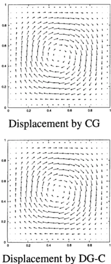
discontinuous $P^{1}-u$ _and continuous

$P^{1}-\hat{u}.$

The results

are

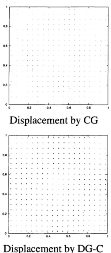
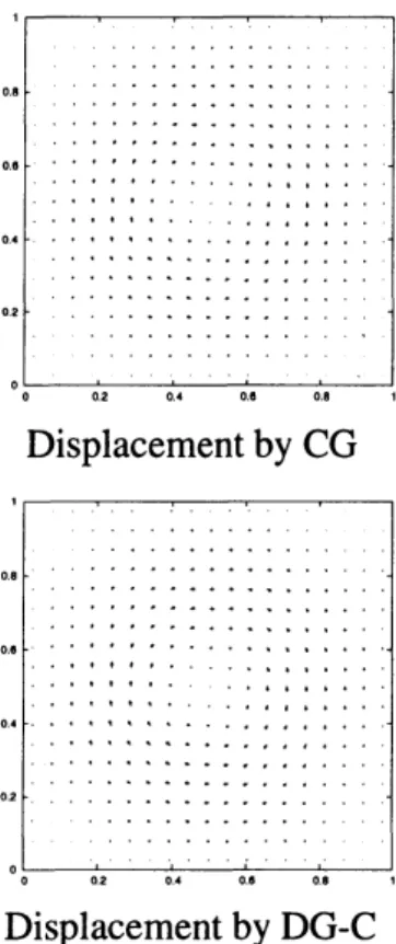
shown in Fig.5 through 8, and

we

can

observe that the results

may

stronglydepend

on

element types. Thatis,whentriangulations

are

coarser,the results based

on

CG and DG-C

are very poor:

the displacements

are

much smaller than the exact one,

whichis very close tothe

ones

basedonDG-D in graphicallevel. The results

are

improved

as

the triangulations become finer, but

we

need much

more

computational costs than using

the DG-D method. Onthe contrary, theresultsbased

on

DG-D

are

robust to the finenessof

triangulations

as

is expected theoretically. It is to be noted that, for smaller $\lambda$ (not shown

here), the differenceisnot

so

severe

and sometimes$CG$ may givebetterresults.

Triangulation 1 Displacementby CG

Displacementby DG-D DisplacementbyDG-C

Triangulation 2 Displacement by CG

Displacementby DG-D Displacement by DG-C

Figure

6:

Triangulation 2andcomputed displacements

Triangulation 3 Displacement by CG

Displacement by DG-D Displacement by DG-C

Triangulation4 Displacement by CG

Displacement by DG-D Displacement by DG-C

Figure 8: Triangulation4 andcomputeddisplacements

10

Concluding remarks

We have surveyed fundamental finite elementmethods for nearly incompressible media. As

a

whole, the mixed methods using the

pressure

$p$

as

well

are

superior to the methods in

displacements(or velocities)only,butitisnotso easyto find nice finiteelement models.

As alternatives, the hybrid DGFEM and theirmixed variants may be promising to

de-rive

more

flexible finite element models that behave nicely in nearly incompressible cases,

although their practical feasibility (cost, size of discretized problems,etc.) mustbecarefully

tested. Finally,

we

have essentially omit the proofs of theoretical results, which must be

completed

as soon

as

possible.

References

[1] Arnold, D.N., On nonconforming linear-constant element for

some

variants of the

Stokesequations. Istit.Lombardo Accad. Sci. Lett. Rend. A01/1993127,

83-93

(1994)

[2] Arnold, D.N., Brezzi, F., Cockburn, B., Marini, L.D.,Unified analysis of discontinuous

Galerkin methods forellipticproblems. SIAM J. Numer. Anal. 39, 1749-1779 (2002)

[3] Brenner, S.C., Scott, L.R., The Mathematical Theory ofFinite Element Methods. 3rd ed.Springer (2008)

[4] Brenner, S.C.,Kom’s inequalities for

piecewise

$H^{1}$

vectorfields. Mathematics of

Com-putation 73, 1067-1087 (2003)

[5] Brezis, H., Functional Analysis, Sobolve Spaces and Partial Differential Equations.

Springer(2011)

[6] Boffi, D., Brezzi, F., Fortin, M., Mixed Finite Element Methods and Applications.

Springer(2013)

[7] Buffa, A., Ortner, C.,Compact embeddings of broken Sobolevspacesandapplications.

IMA J. Numer. Anal. 29,

827-855

$(2\alpha)9$)

[8] Cockbum, B., Gopalakrishnan, J., Lazarov, R., Unifiedhybridizationofdiscontinuous

Galerkin,mixed, andcontinuousGalerkin methodsfor second orderellipticproblems.

SIAM J. Numer. Anal. 47,

1319-1365

(2009)

[9] Egger,H.,Waluga,C.,hp analysis of

a

hybrid DG method for Stokes flow. IMAJoumal

of Numerical Analysis33, 687-721 (2013)

[10] Geuzaine, G. and G. Remacle, J.-F., Gmsh: A3-D finite element mesh generator

with built-in pre-and

post-processing

facilities. Internat. J. Numer. Methods Engrg.

79,

1309-13331

(2009)

[11] Hughes,T.J.R.,TheFiniteElementMethod: Linear Static andDynamicFiniteElement

Analysis.Prentice-Hall (1987)

[12] Kikuchi, F., Rellich-type discrete compactness for

some

discontinuous GalerkinFEM,

JapanJ. Indust. Appl. Math. 29,

269-288

(2012)

[13] Kikuchi, F., Ishii, K., Oikawa, I.,Discontinuous Galerkin FEMofhybrid displacement

type–development ofpolygonalelements_–.Theor. Appl. Mech.Japan.57, 395-404

(2009)

[14] Kikuchi, F., Koyama,D., Strong$L^{p}$

convergence

associated with Rellich-type discrete

compactness for discontinuous Galerkin FEM, JSIAMLetters 6,

25-28

(2014)

[15] Koyama,D., Kikuchi, F., A hybridized discontinuous Galerkin FEM with lifting

oper-ator for plane elasticity problems, Discussionpapers/GraduateSchool

_of

Economics,

Hitotsubashi University, No. 2014-04,2014.

[16] Oikawa, I., A hybridizeddiscontinuous Galerkin method with reduced stabilization. J.

Sci. Comput. toappear.