Panel Data Research Center at Keio University
DISCUSSION PAPER SERIES
DP2014-007 March, 2015
- Policy Evaluation of the Job Café Related Projects –
Isamu Yamamoto*
Yasuhiro Nohara*
【Abstract】
This paper conducts a policy evaluation of the Job Café support programs that had been implemented as the regional active labor market policy for the youth since the 2000s in Japan. First, we estimate job matching function using prefectural panel data to examine whether the efficiency of job matching increased in the target model regions covered by the programs. The results show that the matching efficiency may have increased in the target model regions as a result of the Job Café support programs between FY 2005 and 2007. Next, we conduct a difference-in-differences analysis based on regression model, using household panel data, to examine whether the individual employment probability increased. The results do not show the strong evidence that the probability of regular and non-regular employment increased in the target model regions. Thus, we interpret that while the Job Café support programs may have created employment for Job Café users, the programs did not significantly improved the overall employment environment of the youth in the region.
* Graduate School of Business and Commerce, Keio University
Panel Data Research Center at Keio University Keio University
Active Labor Market Policy and Youth Employment in Japan
∗– Policy Evaluation of the Job Café Related Projects –
Isamu Yamamoto* Yasuhiro Nohara
Keio University Keio University Abstract
This paper conducts a policy evaluation of the Job Café support programs that had been implemented as the regional active labor market policy for the youth since the 2000s in Japan. First, we estimate job matching function using prefectural panel data to examine whether the efficiency of job matching increased in the target model regions covered by the programs. The results show that the matching efficiency may have increased in the target model regions as a result of the Job Café support programs between FY 2005 and 2007. Next, we conduct a difference-in-differences analysis based on regression model, using household panel data, to examine whether the individual employment probability increased. The results do not show the strong evidence that the probability of regular and non-regular employment increased in the target model regions. Thus, we interpret that while the Job Café support programs may have created employment for Job Café users, the programs did not significantly improved the overall employment environment of the youth in the region.
Keywords: Active labor market policy, Youth employment, Matching function, Difference-in-differences analysis, Job Café
* Corresponding Author: [email protected], Tel/Fax: +81-3-5427-1085
The authors deeply appreciate Yoshio Higuchi, Michio Naoi, and Hirotaka Ito for their valuable comments. We are grateful for access to the micro data from the “Keio Household Panel Survey,” provided by the Panel Data Research Center at Keio University, and the prefectural data from the JEPS Statistics, provided by the Ministry of Health, Labor, and Welfare. Any remaining errors are entirely our own.
1
1. Introduction
What effects can we expect for the active labor market policy targeting the youth of specific regions? In this paper, we examine the effect on youth employment of the Job Café support programs, the regional active labor market policy for the youth implemented since the 2000s in Japan, based on prefectural panel data on public job placements and individual household panel data.
The employment environment for the youth has continued to deteriorate in the Japanese labor market since the 1990s, a time known as the employment ice age. The unemployment rate for those between the ages of 15 and 24 shifted between 3 and 5% until the 1980s. However, this rate increased much faster than it did for other age groups after the burst of the bubble economy, reaching approximately 10% by the early 2000s. In addition to the unemployment rate, the non-regular employment rate increased rapidly from the late 1990s and, by the 2000s, one out of three people between the ages of 15 and 24, excluding students, were employed in this category. On the other hand, there were notable differences in the employment environment for the youth among the regions. For example, in 2003, the unemployment rate for those between the ages of 15 and 24 was 7.4% in the Hokuriku region, 12.9% in the Hokkaido region, and 12.7% in the Kyushu and Okinawa regions. As a result, the employment environment for the youth has drawn social attention as an issue that affects the foundations of the economy, such as economic disparity, economic growth, and social security.
Given the circumstances, the government launched intensive active labor market policies for the youth. In April 2003, the “Strategy Council to Foster a Spirit of Independence and Challenge in Youth” was established, in which the members included the Minister of Education, Culture, Sports, Science, and Technology, the
Minister of Economy, Trade, and Industry(hereafter, “METI”), and the State Minister in Charge of Economic and Fiscal Policy. Then, in June of the same year, the “youth independence and challenge plan” was compiled. The plan was cross-ministerial and the scope of the policy incorporated a wide range of fields, such as education, employment, and industry, in order to comprehensively implement measures to address the youth employment issues. Komikawa (2010) and Arai (2006) pointed out that the plan is the first full-scale employment measures for the youth in the post-war era in Japan. Subsequently, several measures targeting youth employment have been established, including the “action plan for the independence and challenges of youth” in December 2004, and the “enhanced action plan for the independence and challenges of youth” in October 2005.
As part of the “youth independence and challenge plan,” which covered a wide range of fields, “Job Cafés” were established as the core of youth employment measures for each region. The Job Cafés are one-stop services for the youth, through measures under the initiative of each region, as a new system to collect actual opinions from the youth and to develop careful and effective measures. Specifically, Job Cafés provide career counseling, job seeking information, and job placement in collaboration with the Public Employment Security Office established together with the Job Cafés. Since the start of the program in 2004, Job Cafés have operated in 46 prefectures, excluding the Kagawa Prefecture.
A number of support programs have been implemented to promote the Job Café program: the “model program,” implemented from FY 2004 through 2006; the “program for the network between youth and SMEs to support the Job Café function,” implemented from FY 2006 through 2007; the “Job Café regional network support program,” implemented from FY 2008 through 2010; the “program for personnel support to respond to the employment situation in SMEs,” implemented
from FY 2009 through 2010; and the “program for promoting the employment environment development in SMEs,” implemented in FY 2011.
Through these support programs, the METI has provided intensive support to specific regions between FY 2004 and 2011. Specifically, the support programs implemented in FY 2009 and 2010, “Job Café regional network support program” and the “program for personnel support to respond to the employment situation in SMEs,” were designed against the deterioration in the employment situation after the bankruptcy of Lehman Brothers and the necessity of improvements in employment in local SMEs. These programs were implemented by entrusting the operations to the Japan Chamber of Commerce and Industry (hereafter “JCCI”), based on SMEs across the country. In addition to the budget allocated by the Ministry of Health, Labour, and Welfare (hereafter “MHLW”) to the Job Cafés across the country, the budget for these related programs was allocated intensively to 15 to 20 target regions selected by the METI and the Japan Chamber of Commerce and Industry. The scale of the budget was JPY 2.5 to 3 billion from the MHLW. In addition, the following additional budgets were allocated: JPY 5 to 7 billion for the “model program;” approximately JPY 1.5 billion for the “program for the network between youth and SMEs to support the Job Café function;” JPY 0.5 to 1.5 billion for the “Job Café regional network support program;” approximately JPY 2 billion for the “program for personnel support to respond to the employment situation in SMEs;” and approximately JPY 1 billion for the “program for promoting the employment environment development in SMEs.”
The Job Café programs can be classified as an active labor market policy (ALMP). In contrast to a passive labor market policy, which has conventionally centered on the payment of unemployment benefits, an ALMP is a policy that aims
to help the unemployed find jobs through occupational training and job placement. ALMPs have been widely implemented since the 1990s, mainly in European countries. The shift from a passive to an active labor market policy was recommended in the “OECD Jobs Strategy” in 1994, as well as in the “Restated OECD Jobs Strategy” in 2006.
However, ALMPs have received some criticism. For example, Boeri and Bruda (1996) cast doubt on the effects of ALMPs by pointing out the possibility of creating a negative signal on the unemployed who participate in the program.1
Furthermore, they note the possibility that the high initial productivity of those who obtained jobs through the program meant they would have found a job by themselves without participating in the program.2 In addition, they point out the
possibility that the overall employment across the labor market may not increase, because employment for those outside the scope of the policy could be crowded out. In response to these criticisms, many studies have examined the effects of ALMPs in the field of labor economics. For example, based on a meta-analysis of 137 experimental studies that examined ALMPs in 19 EU countries, Kluve (2010) finds that the “efficient job search service” has relatively the greatest positive effect on the employment probability among four ALMPs. The ALMPs were the following: (1) occupational training program; (2) employment subsidy system; (3) direct employment in public sectors; and (4) efficient job search service. In addition, Card et al. (2010) conduct a meta-analysis of 97 experimental studies in 26 countries, including countries outside the EU. They find that positive effects can be obtained
1 For example, Burtless (1985) measures the effects of the wage subsidy program in the United
States, finding that the employment probability of workers on the program decreased. A possible interpretation is that companies tend to estimate the productivity of the workers on the program as low and thus, use the program participation as a screening device.
2 Calmfors (1994) refers to this situation as a deadweight loss.
5
in terms of employment and wages using the “job search assistance program” within the “efficient job search service.”3
Although the contents of the Job Café related programs are similar to those of the “efficient job search service,” which Kluve (2010) and Card et al. (2010) show to be effective, it is not obvious that the Job Café related programs are also effective in Japan. To the best of our knowledge, only two academic studies provide an empirical analysis of the effects of Job Café related programs: Takahashi (2005) and Nagase and Mizuochi (2011). Takahashi (2005) estimates the job matching function using monthly panel data by prefecture and by age from the “job/employment placement services statistics” (hereafter, “JEPS Statistics”; MHLW) between July 1996 and August 2004. The study finds no statistically significant result that matching efficiency had improved for the 19–29 age group since the start of Job Café programs. On the other hand, Nagase and Mizuochi (2011) examine whether the increase in the Job Café use ratio in the prefectures improves the probability of regular employment. By using monthly micro data from the “Labour Force Survey” (Ministry of Internal Affairs and Communications) between 2002 and 2007, they find a significant effect for men.
These studies offer no consensus on the positive effects of Job Café programs on youth employment. In addition, while the two studies evaluated the Job Café programs as a whole, they did not examine the extent to which the “model program” and other support programs, which allocate a large amount of the budget to specified regions, had an effect. As described earlier, in Japan, there is a marked
3 The results of these two meta-analyses include many experimental studies on ALMPs for people
other than the youth. Blundel et al. (2002) conduct a study on the efficient job search service for the youth using a matching difference-in-differences analysis of the New Deal for Young People Program implemented since 1998 in the U.K. They find that both male and female program participants who searched for a job while receiving counseling during the four-month gateway period had a higher probability of obtaining employment.
6
difference among regions in youth unemployment rate. Therefore, examining whether the regional ALMP can improve the youth employment should be important when designing future employment policies and regional policies.
Therefore, this paper measures empirically the effects of Job Café support programs classified as ALMPs for the target model regions. Our analysis uses prefectural panel data from the JEPS Statistics and household individual panel data, based on the two studies described earlier. The former data are used to examine whether the implementation of Job Café support programs increased the matching efficiency of public job placement. The latter data are used to examine whether the employment probability for regular and non-regular employment improved.4
Our results can be summarized as follows. First, from the estimation of the job matching function using prefectural panel data, we found an increase in matching efficiency between FY 2005 and 2007 in the Job Café support program target regions (model regions). Next, from the DD analysis using a random effect probit model based on individual panel data, we did not find strong evidence of an increase in the probability of employment for regular and non-regular employment in the model regions. Thus, we point out that although there is a possibility of employment creation for Job Café users through the Job Café support programs, the effects were not significant enough to improve the youth employment environment in the regions as a whole.
The rest of the paper are structured as follows. In Section 2, we outline the Job Café programs as an ALMP and explain our analysis approach. In Section
4 This paper is similar to Boeri and Bruda (1996), which studies whether budgetary injections to
76 regions in the Czech Republic under the active labor market policy in the 1990s yielded a significant result. Boeri and Bruda (1996) report that higher budgets tended to be associated with increased employment.
7
3, we introduce the data and variables used in our analysis and use graphs to show the trends in youth employment. Then, in Section 4, we describe the results of the estimations using the matching function and the employment probability function. Finally, Section 5 concludes the paper with a summary of our results and a description of areas of possible future research.
2. Job Café Programs and Analysis Approach
2.1 Target regions of the support programs and the Job Café target age
Under the “Youth independence and challenge plan,” the Job Café programs are positioned as the core of the youth employment measures for each region. In this paper, we measure the effects of the “model program” in which government supports the selected region’s Job Café programs by designating the specific target regions as the “model regions.”
The model program began in FY 2004 when the Job Café programs started. In all, 15 regions (prefectures) were selected as model regions at that time, with an additional five regions specified in FY 2005 and continuing to FY 2006. The model regions then changed from FY 2007 depending on the type of programs. By FY 2011, when the model program ended, 27 prefectures had been designated at least once as model regions. The list of the model regions is shown in Table 1.
The age of workers covered by the programs varies among regions. Job Café programs specify an upper age limit, usually those under 35. However, the Job Cafés in each region set their own target age to respond flexibly to the regional unique labor market situation. The upper age limit for the different regions is shown in Table 2.
2.2 Analysis approach Estimation of the matching function
We take two approaches to measure the effects of model programs of Job Café. The first approach measures the job matching efficiency in the youth labor market. Specifically, by using the JEPS Statistics as monthly panel data by prefecture,5 we
estimate the job matching function to examine whether the matching efficiency has increased as a result of the model support programs.
As introduced by Petrongolo and Pissarides (2001), we formulate the job matching function as follows.
𝑀𝑀𝑖𝑖𝑖𝑖𝑖𝑖 = 𝛽𝛽1+ 𝐷𝐷𝑖𝑖𝑖𝑖𝑖𝑖𝑻𝑻𝒕𝒕𝒕𝒕𝜷𝜷𝟐𝟐+ 𝛽𝛽3𝐷𝐷𝑖𝑖𝑖𝑖𝑖𝑖+ 𝑻𝑻𝒕𝒕𝒕𝒕𝜷𝜷𝟒𝟒
+𝛽𝛽5𝑈𝑈𝑖𝑖t𝑖𝑖+ 𝛽𝛽6𝑉𝑉𝑖𝑖𝑖𝑖𝑖𝑖+ 𝛽𝛽7𝑑𝑑𝑖𝑖𝑖𝑖+ 𝒅𝒅𝒕𝒕𝜷𝜷𝟖𝟖+ 𝑓𝑓𝑖𝑖 + 𝜀𝜀𝑖𝑖𝑖𝑖𝑖𝑖,
(1)
where 𝑀𝑀𝑖𝑖𝑖𝑖𝑖𝑖 denotes the number employed in prefecture i in month m of fiscal year
t (natural logarithmic value); 𝐷𝐷𝑖𝑖𝑖𝑖𝑖𝑖 is a dummy variable indicating the model
regions under the model programs; 𝑻𝑻𝒕𝒕𝒕𝒕 is a vector of year dummy variables; 𝑈𝑈𝑖𝑖𝑖𝑖𝑖𝑖
denotes the effective number of monthly job seekers (natural logarithmic value); 𝑉𝑉𝑖𝑖𝑖𝑖𝑖𝑖 denotes the effective number of monthly job offers (natural logarithmic value);
𝑑𝑑𝑖𝑖𝑖𝑖 is a dummy variable indicating the period of an economic trough; 𝒅𝒅𝒕𝒕 is a
vector of month dummy variables; 𝑓𝑓𝑖𝑖 is a time-invariant prefecture specific factor;
and 𝜀𝜀𝑖𝑖𝑖𝑖𝑖𝑖 is an error term.
Equation (1) is a Cobb–Douglas matching function in which the residuals
5 In addition to the study by Takahashi (2005), introduced in the preceding section, the studies
estimating the matching function based on the JEPS Statistics include Kambayashi and Mizumachi (2014) and Sasaki (2007).
9
can be identified as a matching efficiency when the number of job seekers and job offers are controlled. By putting fiscal year dummies, model region dummy, and the cross-terms of those dummies in the matching function, we conduct a difference-in-differences (DD) analysis where the coefficients of the cross-terms can be interpreted as the effect of model program.
Since the model programs ended in FY 2012, we set the period from FY 2013 as a base of fiscal year dummies 𝑇𝑇𝑖𝑖𝑖𝑖, so that we can identify the coefficients
of the cross-terms of fiscal year dummies (between FY 2005 and FY 2011) 𝜷𝜷𝟐𝟐 as
the average treatment effect (ATE).6,7 If the coefficients 𝜷𝜷
𝟐𝟐 for FY 2005 to 2011
are significantly positive, we interpret that the matching efficiency was high in the model regions during the period when the model program was implemented, and the Job Café support programs did produce an effect.
In addition, we take into account the possibility that the matching efficiency was increased by the efficient job search and job offers as examined in Petrongolo and Pissarides (2001) and Ohta (2010). Specifically, we allow the coefficients of job seekers 𝑈𝑈𝑖𝑖𝑖𝑖𝑖𝑖 and the job offers 𝑉𝑉𝑖𝑖𝑖𝑖𝑖𝑖 to vary due to the effect of
the model program by estimating the following equation.
𝑀𝑀𝑖𝑖𝑖𝑖𝑖𝑖 = 𝛾𝛾1+ 𝐷𝐷𝑖𝑖𝑖𝑖𝑖𝑖𝑻𝑻𝒕𝒕𝒕𝒕 𝜸𝜸𝟐𝟐+ 𝛾𝛾3𝐷𝐷𝑖𝑖𝑖𝑖𝑖𝑖+ 𝑻𝑻𝒕𝒕𝒕𝒕𝜸𝜸𝟒𝟒
+(𝛾𝛾5+𝐷𝐷𝑖𝑖𝑖𝑖𝑖𝑖∙ 𝑻𝑻𝒕𝒕𝒕𝒕𝜸𝜸𝟔𝟔+ 𝛾𝛾7𝐷𝐷𝑖𝑖+ 𝑻𝑻𝒕𝒕𝒕𝒕𝜸𝜸𝟖𝟖)𝑈𝑈𝑖𝑖t𝑖𝑖
+(𝛾𝛾9+𝐷𝐷𝑖𝑖𝑖𝑖𝑖𝑖∙ 𝑻𝑻𝒕𝒕𝒕𝒕𝜸𝜸𝟏𝟏𝟏𝟏+ 𝛾𝛾11𝐷𝐷𝑖𝑖+ 𝑻𝑻𝒕𝒕𝒕𝒕𝜸𝜸𝟏𝟏𝟐𝟐)𝑉𝑉𝑖𝑖t𝑖𝑖
+𝛾𝛾13𝑑𝑑𝑖𝑖𝑖𝑖+ 𝒅𝒅𝒕𝒕𝜸𝜸𝟏𝟏𝟒𝟒+ 𝑓𝑓𝑖𝑖 + 𝜀𝜀𝑖𝑖𝑖𝑖𝑖𝑖.
(2)
6 Although the model programs started in FY 2004, the data available for our study starts from
January 2005. Therefore, the period between April 2004 and December 2004 is not covered by this analysis.
7 As a priority budget is not allocated to specific regions after the end of support programs, we
assume that any direct policy effects are not seen in FY 2013, and focus on a comparison with FY 2013 after the end of programs.
10
If either 𝜸𝜸𝟔𝟔 or 𝜸𝜸𝟗𝟗 is significantly positive, we interpret this to mean that the model
support programs increased the matching efficiency, particularly through the enhanced intensity of the job search and job offer behaviors.
Estimation of the employment probability function
Another approach to investigate the effects of the model programs is the estimation of the employment probability function using the annual panel data at the individual level from the household panel survey. Specifically, we conduct a DD analysis by estimating the following equation.
𝑌𝑌𝑖𝑖𝑖𝑖 = 𝛿𝛿1+ 𝐷𝐷𝑖𝑖𝑻𝑻𝑖𝑖𝜹𝜹𝟐𝟐+ 𝛿𝛿3𝐷𝐷𝑖𝑖 + 𝑻𝑻𝒕𝒕𝜹𝜹𝟒𝟒+ 𝛿𝛿5𝑆𝑆𝑖𝑖+ 𝑿𝑿𝒊𝒊𝒕𝒕𝜹𝜹𝟔𝟔+ 𝑓𝑓𝑖𝑖 + 𝜀𝜀𝑖𝑖𝑖𝑖, (3)
where 𝑌𝑌𝑖𝑖𝑖𝑖 is a dummy variable indicating employment status of individual i in year
t. Specifically, 𝑌𝑌𝑖𝑖𝑖𝑖 takes the value 1 if the individual is employed as a regular or
non-regular employee. 𝐷𝐷𝑖𝑖 is a model region dummy variable that takes the value 1
if the individual lives in a model region. 𝑻𝑻𝒕𝒕 is a vector of year dummy variables.
𝑆𝑆𝑖𝑖 is a dummy variable indicating a junior or senior high school graduate. 𝑿𝑿𝒊𝒊𝒕𝒕 is a
vector of control variables such as age, spouse dummy, child dummy (1 if having a child under 6), living with parents dummy, the number of people living together, non-work income, GDP growth rate of the prefecture. 𝑓𝑓𝑖𝑖 is a time-invariant
individual specific factor; and 𝜀𝜀𝑖𝑖𝑖𝑖 is an error term.
In the same manner as the equations (1) and (2), we interpret the coefficients of the cross term of the model region dummy and the year dummy variables 𝜹𝜹𝟐𝟐 as indicating the ATE. Since we use the panel data from the household
panel survey as of January of each year, the data for 2004 apply before the model program began in April 2004. Therefore, we set year 2004 as the base for year
dummy variables so that we can compare the years before the model program (2004) and the year after the program (2005~12). Accordingly, if the coefficient of each year between 2005 and 2012 is significant and positive, we interpret this to mean that the employment probability is high in the model regions and that the Job Café support program has a positive effect on the youth employment.
We also estimate the equation (4), in which the cross term of the model region dummy 𝐷𝐷𝑖𝑖 and a vector of year dummy variables 𝑻𝑻𝒕𝒕 are incorporated in
the junior/senior high school graduate dummy 𝑆𝑆𝑖𝑖, to examine whether or not the
effect of the model program differs across the academic background.
𝑌𝑌𝑖𝑖𝑖𝑖 = 𝜃𝜃1+ 𝐷𝐷𝑖𝑖𝑻𝑻𝒕𝒕𝜽𝜽𝟐𝟐+ 𝜃𝜃3𝐷𝐷𝑖𝑖 + 𝑻𝑻𝒕𝒕𝜽𝜽𝟒𝟒
+(𝜃𝜃5+𝐷𝐷𝑖𝑖𝑻𝑻𝒕𝒕𝜽𝜽𝟔𝟔+ 𝜃𝜃7𝐷𝐷𝑖𝑖 + 𝑻𝑻𝒕𝒕𝜽𝜽𝟖𝟖)𝑆𝑆𝑖𝑖 + 𝑿𝑿𝒊𝒊𝒕𝒕𝜽𝜽𝟗𝟗+ 𝑓𝑓𝑖𝑖+ 𝜀𝜀𝑖𝑖𝑖𝑖. (4)
We estimate the equations (3) and (4) as a random effect probit model.
3. Data
3.1 Data and variables
The data used in this paper are the prefectural panel data from the JEPS Statistics and individual panel data from the Keio Household Panel Survey (KHPS).
The JEPS Statistics are released by the MHLW at the end of every month, and provide an outline of the job search, job offers, and employment situations, handled by the Public Employment Security Offices (excluding new graduates). The data available for this paper are by prefecture and by age group, and further narrowed down according to the Job Café target age, which varies among
prefectures, as shown in Table 2. Kagawa Prefecture, which does not have a Job Café, is excluded from the sample. The data period is between January 2005 and December 2013. Although we should use the data before 2004, when the model programs began, we are not able to use the data before 2004 due to the data availability. We thus use the data since 2005 only.
The variables used in the estimation are as follows: the number of monthly new employment, 𝑀𝑀𝑖𝑖𝑖𝑖𝑖𝑖; the active number of monthly job seekers, 𝑈𝑈𝑖𝑖𝑖𝑖𝑖𝑖; the active
number of monthly job offers, 𝑉𝑉𝑖𝑖𝑖𝑖𝑖𝑖; the model region dummy, 𝐷𝐷𝑖𝑖𝑖𝑖𝑖𝑖; the fiscal year
dummy, 𝑻𝑻𝒕𝒕𝒕𝒕; as well as the other variables explained in the equations (1) and (2).
The basic statistics are shown in Table 3.
The KHPS is the longitudinal household survey conducted at the end of January each year from 2004 for individuals randomly extracted from men and women between 20 and 69. We use the data from the survey between 2004 and 2014, during which the GDP growth rate, a control variable for the economic situation in each prefecture, was available to us. In the same manner as the JEPS Statistics, the sample is selected according to the Job Café target ages, which vary among prefectures.
From the KHPS, we can get the information whether the individual is working or not, employed or self-employed, a regular worker or non-regular worker (contract worker, part-time, temporary worker from an agency, fixed-term employee). We focus on the employment dummy, regular employment dummy, and non-regular employment dummy. The basic statistics of the KHPS are shown in Table 4.
3.2 Data Overview: Transition of the youth labor market from 2004
Prior to the DD analysis, this section graphically shows the basic trends in youth
employment provided by the data. First, we present an overview of major trends in the youth labor market at the prefectural level using the JEPS Statistics. Figures 1 to 3 show the annual transition of the average number of monthly new employment, the number of monthly job seekers, and the number of monthly job offers for the Job Café target ages, respectively. The vertical lines for each marker in the figure show the 95% confidence intervals.
In Figure 1, we see that the number of monthly new employment in the model regions is greater than that in non-model regions in every fiscal year. Furthermore, it seems that the gap increased from FY 2009 through FY 2010. On the other hand, the number of job seekers in Figure 2 shows no significant gap until FY 2009. However, the number is greater in the model regions from FY 2010 through FY 2011. In addition, the number of job offers, shown in Figure 3, is greater in the model regions from FY 2010 onward though it is greater in the non-model regions until FY 2009.
These results imply that the number of job seekers and job offers through the Public Employment Security Offices has increased since FY 2010, and that this may have increased the number of new employment. On the other hand, the number of new employment was greater than that in the non-model regions although the number of job offers was smaller in the model regions until FY 2009. Therefore, we can point out the possibility that the Job Café support programs increased the matching efficiency.
From these figures, however, it is hard for us to judge whether the relative increase in the number of new employment in the model regions was caused by the increase in inputs, such as job seekers and job offers, or whether it was due to better matching efficiency. In addition, the confidence intervals indicate that the statistical significance of the gap observed in these figures is not necessarily strong.
Furthermore, we have not controlled for other factors. Therefore, to examine whether the Job Café support programs indeed increased the matching efficiency, we conduct a DD analysis as described in the next section.
Figures 4 and 5 present the transition of employment rate for male and female, respectively, in the model regions and non-model regions. According to these figures, the employment rate for male in the model regions (Figure 4) tends to be lower than that in the non-model regions. It seems that the gap increased since 2008, which coincides with the end of the model programs with the largest budgets. Therefore, it is likely that the injection of funds through the model programs increased the employment rate for male in the model regions. On the other hand, the employment rate for female, as shown in Figure 5, decreased in the model regions until 2008, then increased until 2010, before decreasing until 2012. We examine these trends in the DD analysis described in the next section.
4. Estimation Results
4.1 Matching function
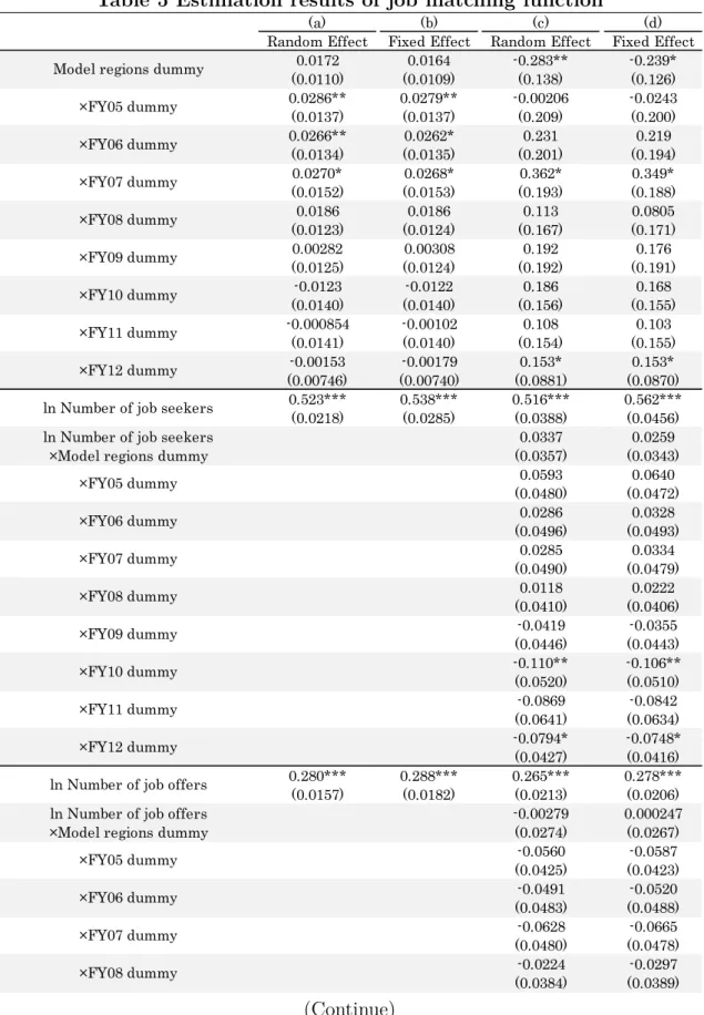
The estimation results of the equations (1) and (2) are shown in Table 5. Columns (a) to (b) show the estimation results for the equation (1), and columns (c) to (d) show that for the equation (2). The result of the Hausman test is also listed in Table 5, which shows that the fixed effect model is supported for both the equations (1) and (2).
First, focusing on the row (b), supported by the Hausman test, we find that the coefficients of the number of job seekers and job offers are significantly
positive,8 and that the coefficients of the cross term of the model region dummy
and the fiscal year dummies between FY 2005 and FY 2007 are also significantly positive. According to this result, we can point out that the matching efficiency increased between FY 2005 and FY 2007 in the model regions. The coefficients indicate that the matching efficiency increased in the model regions by 3 % because of these programs.
Next, focusing on row (d), we find that the coefficient of the cross term of the model region dummy and the fiscal year dummy for FY 2007 is significantly positive, although the coefficients of the cross term of the FY 2005 dummy and FY 2006 dummy are no longer statistically significant. In addition, most of the coefficients of the cross term for the number of job seekers are not statistically significant, and the cross term of the FY 2010 dummy and the FY 2012 dummy are significantly negative. On the other hand, although the coefficient of the cross term of the number of job offers for FY 2010 is significantly positive, it is not statistically significantly different from zero for the other fiscal years. These results indicate that the matching efficiency in the model regions between FY 2005 and FY 2007 increased, but we could not specify that the increase in the efficiency was caused either by the job offer actions or by the job search actions.
As for the reason why we observe the increase in the matching efficiency only in the FY 2005, 2006, and 2007, we can point out the followings. The first reason is the large budget. The budget of the model programs implemented between FY 2004 and 2006 was approximately 5 to 7 billion yen, which was three to four times larger than that implemented from FY 2007 onward. Since the support of a
8 The total of the coefficient of the number of job seekers and the job offers (both natural
logarithmic values) is between 0.8 and 0.9, which is almost consistent with the estimation results of the preceding studies, including Takahashi (2005).
16
budget at a certain minimum level is necessary to improve the matching efficiency, this may be why the policy effects appear mainly in the period between 2004 and 2006.
A second possible reason is the difference among the programs and the implementation bodies. In FY 2008, the program changed from the “program for the network between youth and SMEs to support Job Café function” to the “Job Café regional network support program.” In addition, in FY 2009 and 2010, the support provider changed from the METI to the JCCI. These changes in the content of the programs and the support systems, owing to the changes in programs and implementation bodies, may have blocked the expected increase in matching efficiency.
A third possible reason is external factors such as the economic downturn. In Figure 3, the number of job offers exhibits a rapid decrease from FY 2007, and began recovering from FY 2010. However, it has still not recovered to its level prior to FY 2006. Conversely, the number of job seekers has increased since FY 2008 and maintained a high level between FY 2009 and 2011. Thus, it is likely that the job matching function for the youth deteriorated because employment agencies such as “Hello Work (the Public Employment Security Office)” became crowded with many job seekers owing to the financial crisis.
4.2 Employment probability function
Tables 6 and 7 provide the estimation results of the equations (3) and (4). Table 6 is the estimation results for men and Table 7 for women, and the both tables show the marginal effect. In each table, columns (a) to (c) show the estimation results of equation (3) and columns (d) to (f) show the estimation results of equation (4).
Focusing on the results for male in Table 6, we find no significant marginal
effects of the cross term of the model region dummy and the year dummies, as well as the cross term of the junior/senior high school-graduate dummy, regarding the employment rate and regular employment rate. In addition, we see that the marginal effects of the cross term of the model regions dummy for 2005 dummy and 2012 dummy are significantly negative. Furthermore, the cross term of the model regions dummy and the year dummy or the junior/senior high school- graduate dummy are significantly negative.
Based on these results, we cannot say that employment situation for the young male worker improved during the period of Job Café support program implementation in the model regions, if any, there was a limited improvement.
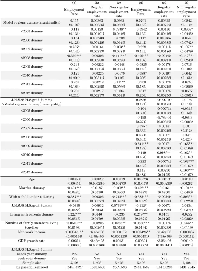
Table 7, showing the estimation results for female, indicates that the marginal effects of the cross term of the model regions dummy and 2007 and 2008 dummies are significantly negative. The table also shows that the marginal effects of the cross term of the junior/senior high school graduate dummy and each year dummy from 2009 through 2012 are significantly negative. Thus, the positive effects of the Job Café support programs on the young female employment cannot be confirmed from these estimation results.
5. Concluding remarks
In this paper, we examined the influence of the ALMP, Job Café support programs, on the youth regional employment by estimating the matching function and the employment probability function. The estimations of the matching function based on prefectural panel data indicate that the Job Café support programs increased the matching efficiency in the model regions between FY 2005 and 2007. However,
the estimations of the employment probability function do not show the evidence of the improvement in the probability of regular and non-regular employment in the model regions. Based on these two results, we could conclude that the Job Café support programs possibly created the employment for Job Café users, but the effect was not significant enough to improve the overall employment environment of the youth for the model regions.
The different results for the matching function and employment probability function can be interpreted as follows. First, there is a possibility that not many workers receive the benefit of the programs because the Job Café programs are based on the employment agencies such as “Hello Work (the Public Employment Security Office).” The use rate of the Hello Work is low, as shown in the Survey on Employment Trends (MHLW, 2008), which indicates that only about 23% of those newly employed in the year used the Hello Work, including its Internet services. Therefore, even if the Job Café programs have a positive effect for their users in terms of matching efficiency, it is likely that the effect did not spread to all workers living in the regions because of the low use rate.
Second, as described in the Section 1, there is a criticism of the ALMP in which even if the employment probability of Job Café users increased, it may be the case that the employment probability of non-users decreased because of a crowding out effect. Since household panel data includes randomly selected individuals in each region, the estimation results may reflect the overall influence including the crowding out.
References
Blundell, Richard, Monica Costa Dias, Costas Meghir, and John van Reenen (2004): “Evaluating the employment impact of a mandatory job search program,” Journal of the European Economic Association, 2(4), pp.569-606.
Boeri, Tito and Michael C. Bruda (1996): “Active labor market policies, job matching and the Czech miracle,” European Economic Review, 40(3-5), 805-817.
Burtless, Gary (1985): “Are targeted wage subsidies harmful? Evidence from a wage voucher experiment,” Industrial and Labor Relations Review, 39(1), pp.105-114.
Calmfors, Lars (1994): “Active labour market policy and unemployment – a framework for the analysis of crucial design features,” OECD Economic Studies, No. 22.
Card, David, Jochen Kluve, and Andrea Weber (2010): “Active labor market policy evaluations: A meta-analysis,” NBER Working Paper, No. 16173, Issued in July 2010.
Kluve, Jochen (2010): “The effectiveness of European active labor market programs,” Labour Economics, 17(6), 904-918.
Petrongolo, Barbara and Christopher A. Pissarides (2001): “Looking into the black box: A survey of the matching function,” Journal of Economic Literature, 38, pp.390-431.
Arai, Naoki (2006): “A fundamental study of young person employment policy in region: As a case Job Café ‘Young person of Gunma Prefecture finding employment support center,’” Bulletin of Takasaki University of Health and Welfare, 5, pp.169-180. (in Japanese)
Ohta, Souichi (2010): The economics of youth employment, Nikkei Publishing Inc. (in Japanese)
Kambayashi, Ryo and Mizumachi, Yuichiro (2014): “Policy evaluation on Worker Dispatching Act,” The Japanese Journal of Labour Studies, 56(1), pp.64-82. (in Japanese)
Komikawa, Koichiro (2010): “Trends and issues on youth policies after the ‘plan for independence and challenges of youth:’ Focusing on career education policy,” The Japanese Journal of Labour Studies, 52(9), pp.17-26. (in Japanese)
Sasaki, Masaru (2007): “Measuring efficiency of matching and an incentive to search through the Public Employment Agency in Japan,” The Japanese Journal of Labour Studies, 49(10), pp.15-31. (in Japanese)
Takahashi, Yoko (2005): “Current situation of ‘Job Cafés’ as employment support by municipalities,” The Japanese Journal of Labour Studies, 47(6), pp.56-67. (in Japanese)
Nagase, Nobuko and Mizuochi, Masaaki (2011): “Temporary to permanent employment, the effect of economic recovery, the previous work experiences and the local placement office to the youth employment in Japan,” Journal of Social Sciences and Family Studies, 18, pp.27-45. (in Japanese)
Table 1 List of model regions
Table 2 Upper age limit of the programs in each regions
FY Program name Target regions (Prefecture)
FY2004 Model program Hokkaido, Aomori, Iwate, Gunma, Chiba, Ishikawa, Gifu, Kyoto, Osaka,Shimane, Yamaguchi, Ehime, Fukuoka, Nagasaki, Okinawa FY2005 Model program Hokkaido, Aomori, Iwate, Gunma, Chiba, Ishikawa, Gifu, Kyoto, Osaka,Shimane, Yamaguchi, Ehime, Fukuoka, Nagasaki, Okinawa, Miyagi, Ibaraki,
Niigata, Fukui, Oita FY2006
Model program Program for the network between youth and SMEs to support Job Caf
é function
Hokkaido, Aomori, Iwate, Gunma, Chiba, Ishikawa, Gifu, Kyoto, Osaka, Shimane, Yamaguchi, Ehime, Fukuoka, Nagasaki, Okinawa, Miyagi, Ibaraki, Niigata, Fukui, Oita
FY2007
Model program Program for the network between youth and SMEs to support Job Caf
é function
Hokkaido, Aomori, Iwate, Gunma, Chiba, Ishikawa, Gifu, Kyoto, Osaka, Shimane, Yamaguchi, Ehime, Nagasaki, Okinawa, Miyagi, Ibaraki, Niigata, Fukui, Oita, Hiroshima
FY2008 Job Café regional network supportprogram Hokkaido, Aomori, Iwate, Gunma, Chiba, Ishikawa, Gifu, Kyoto, Osaka,Shimane, Yamaguchi, Ehime, Nagasaki, Okinawa, Miyagi, Ibaraki, Niigata, Fukui, Oita, Hiroshima
Job Café regional network support
program Aomori, Miyagi, Ibaraki, Gunma, Ishikawa, Wakayama, Yamaguchi, Ehime,Oita, Kagoshima, Okinawa Program for personnel support to
respond to the employment situation in SMEs
Hokkaido, Iwate, Tochigi, Chiba, Kyoto, Osaka, Hiroshima, Nagasaki, Kumamoto
Job Café regional network support program
Aomori, Miyagi, Ibaraki, Iwate, Gunma, Ishikawa, Aichi, Wakayama, Yamaguchi, Ehime, Oita, Kagoshima, Okinawa
Program for personnel support to respond to the employment
situation in SMEs Hokkaido, Tochigi, Chiba, Kyoto, Osaka, Hiroshima, Nagasaki, Kumamoto FY2011 Program for promoting theemployment environment
development in SMEs
Hokkaido, Aomori, Iwate, Miyagi, Ibaraki, Tochigi, Gunma, Chiba, Ishikawa, Gifu, Aichi, Kyoto, Osaka, Nara, Wakayama, Hiroshima, Yamaguchi, Ehime, Nagasaki, Kumamoto, Oita, Okinawa
FY2012
onword No support provided from the Ministry of Economy, Trade and Industry to specific regions FY2009
FY2010
Target age Prefecture
29 or younger Fukuoka 34 or younger
(under 35) Tokyo, Gifu, Mie, Kyoto, Osaka, Iwate, Fukushima, Tochigi, Toyama,Ishikawa, Shiga, Nara, Wakayama, Kumamoto, Oita, Kagoshima 39 or younger
(under 40) Ibaraki, Chiba, Kanagawa, Fukui, Yamanashi, Shizuoka, Hyogo,Yamaguchi, Ehime, Kochi, Saitama, Okayama, Nagasaki 44 or younger Hokkaido, Miyazaki, Niigata, Nagano, Hiroshima, Okinawa, Aomori,Yamagata, Gunma, Aichi, Tottori, Shimane, Tokushima, Saga
Table 3 Basic statistics: JEPS
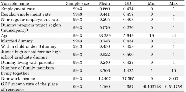
Table 4 Basic statistics: KHPS
Variable name Sample size Mean SD Min Max
The number of monthly new
employment 4968 1851.765 1118.031 408 6531
The number of monthly job
seekers 4968 24760.560 20116.870 4875 106987
The number of monthly job
offers 4968 20719.450 22251.330 3059 176811
Program target region
dummy (prefecture) 4968 0.472 0.499 0 1
Economic trough dummy 4968 0.185 0.388 0 1
Variable name Sample size Mean SD Min Max
Employment rate 9943 0.660 0.474 0 1
Regular employment rate 9943 0.441 0.497 0 1
Non-regular employment rate 9943 0.205 0.403 0 1
Dummy program target region
(municipality) 9943 0.079 0.270 0 1
Age 9943 33.239 5.649 19 44
Married dummy 9943 0.748 0.434 0 1
With a child under 6 dummy 9943 0.456 0.498 0 1
Junior high school-/senior high
school-graduate dummy 9943 0.522 0.500 0 1
Dummy living with parents 9943 0.240 0.427 0 1
Number of family members
living together 9943 3.766 1.425 1 10
Non-work income 9943 12.407 77.595 0 3000
GDP growth rate of the place
of residence 9943 1.169 2.657 -9.193148 9.514758
Table 5 Estimation results of job matching function
(Continue)
(a) (b) (c) (d)
Random Effect Fixed Effect Random Effect Fixed Effect
0.0172 0.0164 -0.283** -0.239* (0.0110) (0.0109) (0.138) (0.126) 0.0286** 0.0279** -0.00206 -0.0243 (0.0137) (0.0137) (0.209) (0.200) 0.0266** 0.0262* 0.231 0.219 (0.0134) (0.0135) (0.201) (0.194) 0.0270* 0.0268* 0.362* 0.349* (0.0152) (0.0153) (0.193) (0.188) 0.0186 0.0186 0.113 0.0805 (0.0123) (0.0124) (0.167) (0.171) 0.00282 0.00308 0.192 0.176 (0.0125) (0.0124) (0.192) (0.191) -0.0123 -0.0122 0.186 0.168 (0.0140) (0.0140) (0.156) (0.155) -0.000854 -0.00102 0.108 0.103 (0.0141) (0.0140) (0.154) (0.155) -0.00153 -0.00179 0.153* 0.153* (0.00746) (0.00740) (0.0881) (0.0870) 0.523*** 0.538*** 0.516*** 0.562*** (0.0218) (0.0285) (0.0388) (0.0456)
ln Number of job seekers 0.0337 0.0259
×Model regions dummy (0.0357) (0.0343)
0.0593 0.0640 (0.0480) (0.0472) 0.0286 0.0328 (0.0496) (0.0493) 0.0285 0.0334 (0.0490) (0.0479) 0.0118 0.0222 (0.0410) (0.0406) -0.0419 -0.0355 (0.0446) (0.0443) -0.110** -0.106** (0.0520) (0.0510) -0.0869 -0.0842 (0.0641) (0.0634) -0.0794* -0.0748* (0.0427) (0.0416) 0.280*** 0.288*** 0.265*** 0.278*** (0.0157) (0.0182) (0.0213) (0.0206)
ln Number of job offers -0.00279 0.000247
×Model regions dummy (0.0274) (0.0267)
-0.0560 -0.0587 (0.0425) (0.0423) -0.0491 -0.0520 (0.0483) (0.0488) -0.0628 -0.0665 (0.0480) (0.0478) -0.0224 -0.0297 (0.0384) (0.0389) ×FY05 dummy ×FY06 dummy ×FY07 dummy ×FY08 dummy ×FY07 dummy ×FY08 dummy ×FY09 dummy ×FY10 dummy ×FY11 dummy ×FY12 dummy ×FY12 dummy ×FY11 dummy ×FY10 dummy ×FY09 dummy ×FY05 dummy ×FY06 dummy Model regions dummy
ln Number of job seekers
ln Number of job offers ×FY05 dummy ×FY06 dummy ×FY07 dummy ×FY08 dummy
Notes: 1. Numbers in parentheses are robust standard errors.
2. ***, **, and * indicate statistical significance at the 1%, 5%, and 10 % levels, respectively.
3. Base for fiscal year dummies is 2013.
0.0250 0.0203 (0.0353) (0.0352) 0.0956* 0.0940* (0.0509) (0.0501) 0.0791 0.0770 (0.0615) (0.0608) 0.0653 0.0606 (0.0430) (0.0415) ln Number of effective job seekers
×each FY dummy No No Yes Yes
ln Number of effective job offers
×each FY dummy No No Yes Yes
Each FY dummy Yes Yes Yes Yes
Economic trough dummy Yes Yes Yes Yes
Month dummy Yes Yes Yes Yes
-0.702** -0.925** -0.497* -1.065** (0.281) (0.387) (0.275) (0.399) Hausman(prob>chi2) Sample size 4,968 4,968 4,968 4,968 Adj-R2 0.864 0.864 0.868 0.873 ×FY11 dummy ×FY12 dummy ×FY09 dummy ×FY10 dummy Constant 0.0000 0.0000 25
Table 6 Estimation results of the employment probability function: Male
Notes: 1. Numbers are marginal effect and numbers in parentheses are robust standard errors. 2. ***, **, and * indicate statistical significance at the 1%, 5%, and 10 % levels, respectively.
(a) (b) (c) (d) (e) (f) Employment Rate Regular employment rate Non-regular employment rate Employme nt Rate Regular employment rate Non-regular employment rate -0.00100 -0.0253 0.00186 -0.000553 0.0115 -0.00146* - (0.0453) (0.00376) (0.00742) (0.0210) (0.000833) 0.000769 0.0217 -0.00157* 0.000404 0.0207 -0.00130* (0.0100) (0.0286) (0.000840) (0.00528) (0.0280) (0.000717) 0.000505 0.0189 -0.00144 -0.0122 -0.00897 -0.00120* (0.00612) (0.0244) (0.000877) (0.101) (0.0444) (0.000684) 0.000704 0.00739 -0.000154 0.000598 0.000304 -0.000808 (0.00906) (0.0222) (0.00269) (0.00781) (0.0324) (0.00105) 0.000498 0.0183 -0.00144 -0.000437 0.0165 -0.00122* (0.00613) (0.0240) (0.000925) (0.00513) (0.0233) (0.000672) 0.000769 0.0185 0.00348 0.000600 0.0175 -0.000406 (0.0101) (0.0244) (0.0104) (0.00780) (0.0242) (0.00248) 0.000549 0.0168 -0.000123 0.000338 0.0177 -0.00107 (0.00684) (0.0228) (0.00392) (0.00467) (0.0245) (0.000794) -0.00373 0.00937 -0.000952 -0.0309 0.0186 -0.00132* (0.0404) (0.0263) (0.00196) (0.230) (0.0255) (0.000729) -0.00135 0.0209 -0.00171* -0.0118 0.0194 -0.00130* (0.0152) (0.0277) (0.000902) (0.0977) (0.0265) (0.000717) J.H.S./S.H.S.grad dummy 0.000242 -0.103 0.0829
×Model regions dummy(municipality) (0.00299) (0.155) (0.0991) 0.000717 0.00782 0.0448 (0.00948) (0.0322) (0.0988) 0.000728 0.0213 0.0113 (0.00966) (0.0298) (0.0394) 0.000418 0.0168 0.0166 (0.00477) (0.0254) (0.0510) 0.000699 0.0183 -0.00125* (0.00921) (0.0266) (0.000694) 0.000708 0.0178 -0.00124* (0.00940) (0.0297) (0.000690) -0.000763 -0.0946 -0.00122* (0.0129) (0.241) (0.000682) 0.000721 -0.590 0.999*** (0.00959) (0.459) (0.000895) 0.000718 0.0211 0.358 (0.00955) (0.0296) (0.281) Age -9.32e-05 0.00221 -0.000479** -8.20e-05 0.00226 -0.000382**
(0.00114) (0.00226) (0.000222) (0.00101) (0.00240) (0.000185) Married dummy 0.0132 0.157 -0.00885 0.0122 0.158 -0.00755
(0.120) (0.123) (0.00581) (0.113) (0.126) (0.00508) With a child under 6 dummy 0.00103 0.0239 -0.000312 0.000971 0.0218 -9.80e-05 (0.0123) (0.0274) (0.00121) (0.0117) (0.0259) (0.000939) J.H.S./S.H.S.grad dummy -0.00120 -0.00769 -0.00222* -0.000549 0.00596 -0.00181
(0.0139) (0.0161) (0.00128) (0.00639) (0.0158) (0.00127) Living with parents dummy -0.000101 -0.0177 0.00251 -2.26e-06 -0.0151 0.00207
(0.00192) (0.0276) (0.00234) (0.000917) (0.0255) (0.00198) -0.000854 -0.0125 -0.000392 -0.000829 -0.0124 -0.000329 (0.0100) (0.0138) (0.000434) (0.00979) (0.0141) (0.000349) Non-work income -8.06e-07 -1.83e-05 1.02e-06 -7.43e-07 -1.66e-05 5.30e-07
(1.00e-05) (2.96e-05) (1.57e-06) (9.29e-06) (2.84e-05) (1.26e-06) GDP growth rate 8.93e-05 0.000852 0.000195 8.87e-05 0.00112 0.000122 (0.00107) (0.00172) (0.000163) (0.00107) (0.00193) (0.000124) J.H.S./S.H.S.grad dummy
×each year dummy No No No Yes Yes Yes
each year dummy Yes Yes Yes Yes Yes Yes
Sample size 4,535 4,535 4,535 4,535 4,535 4,535 log pseudolikelihood -1303.2552 -1574.071 -802.90645 -1293.4415 -1560.3689 -791.57082 ×2009 dummy ×2010 dummy ×2011 dummy ×2012 dummy
Model regions dummy(municipality)
Number of family members living together ×2006 dummy ×2005 dummy ×2005 dummy ×2006 dummy ×2007 dummy ×2008 dummy ×2012 dummy ×2011 dummy ×2010 dummy ×2009 dummy ×2008 dummy ×2007 dummy 26
Table 7 Estimation results of the employment probability function: Female
Notes: 1. Numbers are marginal effect and numbers in parentheses are robust standard errors. 2. ***, **, and * indicate statistical significance at the 1%, 5%, and 10 % levels, respectively.
(a) (b) (c) (d) (e) (f) Employment Rate Regular employment rate Non-regular employment rate Employment Rate Regular employment rate Non-regular employment rate 0.115 0.00363 0.0962 0.0701 0.00395 0.0842 (0.102) (0.00656) (0.0860) (0.156) (0.00797) (0.110) -0.118 0.00120 -0.0938** -0.0942 0.00130 -0.0868* (0.136) (0.00401) (0.0446) (0.139) (0.00416) (0.0445) -0.154 0.000703 -0.0709 -0.117 0.000465 -0.0546 (0.128) (0.00428) (0.0645) (0.142) (0.00385) (0.0742) -0.237* -0.00161 -0.103** -0.228 -0.00115 -0.107** (0.143) (0.00233) (0.0481) (0.146) (0.00186) (0.0479) -0.399*** -0.00206 -0.141*** -0.409*** -0.00140 -0.147*** (0.110) (0.00280) (0.0328) (0.107) (0.00211) (0.0243) -0.243 -0.00222 -0.0448 -0.0825 -0.00178 0.0716 (0.155) (0.00304) (0.0885) (0.146) (0.00261) (0.136) -0.121 -0.00225 -0.0170 -0.0887 -0.00197 0.0642 (0.201) (0.00311) (0.116) (0.206) (0.00288) (0.165) -0.257 -0.00212 -0.111** -0.230 -0.00170 -0.0716 (0.183) (0.00290) (0.0566) (0.185) (0.00249) (0.0856) -0.291 -0.00217 -0.104 -0.317 -0.00175 -0.0607 (0.213) (0.00297) (0.0641) (0.209) (0.00256) (0.0961) J.H.S./S.H.S.grad dummy 0.0836 -0.000790 0.0175
×Model regions dummy(municipality) (0.171) (0.00175) (0.110) -0.104 -0.000714 -0.0313 (0.301) (0.00198) (0.150) -0.190 -9.78e-05 -0.0843 (0.274) (0.00357) (0.0993) -0.0757 -0.00147 0.101 (0.339) (0.00249) (0.212) 0.0600 -0.00177 0.347 (0.343) (0.00261) (0.421) -0.541*** -0.00171 -0.165*** (0.127) (0.00250) (0.0169) -0.149 0.998*** -0.162*** (0.461) (0.00255) (0.0167) -0.222 -0.000746 -0.163*** (0.465) (0.00328) (0.0167) 0.118 0.00260 -0.163*** (0.484) (0.0122) (0.0167) Age 0.000580 -0.000235 0.00119 0.000526 -0.000185 0.00109 (0.00454) (0.000284) (0.00273) (0.00457) (0.000238) (0.00267) Married dummy -0.401*** -0.0187 -0.102** -0.402*** -0.0161 -0.101** (0.0428) (0.0218) (0.0468) (0.0427) (0.0200) (0.0458) With a child under 6 dummy -0.387*** -0.00306 -0.212*** -0.382*** -0.00249 -0.205***
(0.0392) (0.00377) (0.0232) (0.0392) (0.00328) (0.0229) J.H.S./S.H.S.grad dummy -0.0635 -0.00932 0.0761*** -0.112* -0.00671 0.0434
(0.0488) (0.0105) (0.0292) (0.0605) (0.00839) (0.0371) Living with parents dummy 0.222*** 0.0146 -0.0235 0.219*** 0.0141 -0.0292 (0.0518) (0.0179) (0.0335) (0.0521) (0.0179) (0.0322) -0.0540*** -0.00205 0.0255** -0.0536*** -0.00176 0.0255** (0.0193) (0.00261) (0.0122) (0.0194) (0.00238) (0.0119) Non-work income -0.000451** -6.45e-06 -0.000172 -0.000426** -5.42e-06 -0.000165
(0.000194) (8.98e-06) (0.000123) (0.000191) (7.95e-06) (0.000119) GDP growth rate 0.00294 -2.43e-05 0.00131 0.00304 -3.26e-05 0.00149
(0.00600) (0.000166) (0.00388) (0.00602) (0.000141) (0.00378) J.H.S./S.H.S.grad dummy
×each year dummy No No No Yes Yes Yes
each year dummy Yes Yes Yes Yes Yes Yes
Sample size 5,408 5,408 5,408 5,408 5,408 5,408 log pseudolikelihood -2447.4927 -1523.5508 -2509.598 -2441.1537 -1513.3294 -2492.7845 ×2008 dummy ×2009 dummy ×2010 dummy ×2011 dummy ×2012 dummy
Number of family members living together ×2010 dummy ×2011 dummy ×2012 dummy ×2005 dummy ×2006 dummy ×2007 dummy
Model regions dummy(municipality) ×2005 dummy ×2006 dummy ×2007 dummy ×2008 dummy ×2009 dummy 27
Figure 1 Annual transition of the number of monthly new employment
Notes: The vertical lines in the figures represent the 95% confidence interval.
Figure 2 Annual transition of the number of monthly job seekers
Notes: The vertical lines in the figures represent the 95% confidence interval. 28
Figure 3 Annual transition of the number of monthly job offers
Notes: The vertical lines in the figures represent the 95% confidence interval.
Figure 4 Annual transition of employment rate: Male
Notes: The vertical lines in the figures represent the 95% confidence interval.
Figure 5 Annual transition of employment rate: Female
Notes: The vertical lines in the figures represent the 95% confidence interval.