Pairing-based cryptography and construction of
pairing-friendly elliptic and hyperelliptic
curves
著者
Komuta Aya
内容記述
学位授与大学: Osaka Prefecture University(大阪
府立大学), 学位の種類: 博士(理学), 学位記番号:
論理第83号, 学位授与年月日: 2010-03-31, 指導教
員: 高橋哲也.
大阪府立大学博士論文
Pairing-based cryptography and construction of
pairing-friendly elliptic and hyperelliptic curves
大阪府立大学大学院 理学系研究科
博士後期課程 情報数理科学専攻
小牟田 綾
Contents
1 Introduction 1
2 Preliminary 3
2.1 Definition of cryptosystem . . . 3
2.2 The public key cryptography . . . 3
3 Elliptic and hyperelliptic curves 7 3.1 Elliptic curves . . . 7
3.2 Elliptic curve cryptosystems . . . 8
3.3 Hyperelliptic curves . . . 10
3.4 The Weil Pairing . . . 13
3.5 The Weil pairing on elliptic curves . . . 13
4 Constructing pairing-friendly elliptic curves 16 4.1 Pairing based cryptosystem . . . 16
4.2 Pairing-friendly elliptic curves . . . 18
4.3 Construction of pairing-friendly elliptic curves . . . 19
4.4 Constructing pairing friendly elliptic curves for the embedding degree 2n, n is odd prime . . . 23
4.5 Our construction . . . 23
4.6 Table of ρ-values (as p, ℓ→ ∞) . . . 24
5 Pairing-friendly elliptic curves with small security loss by Cheon’s algorithm 26 5.1 Pairing-related problems . . . 26
5.2 Cheon’s algorithm and its improvement . . . 27
5.3 The Effect of Cheon’s algorithm for constructing pairing-friendly el-liptic curves . . . 28
5.4 How to reduce a security loss of a cyclotomic family . . . 30
5.6 Our result . . . 32 5.7 Examples . . . 34
6 Pairing-based cryptography on hyperelliptic curves 37
6.1 The Jacobian of hyperelliptic curves and the Weil pairing . . . 37 6.2 The definition of pairing-friendly hyperelliptic curves . . . 38
7 The Jacobstahl sum and the order of the Jacobian group 39
7.1 The Jacobstahl sum . . . 39 7.2 The Jacobstahl sum and the number of rational points of Hh,τ,c . . . 41
7.3 The order of the Jacobian group for H5,0,c . . . 42 7.4 The order of the Jacobian group of H8,1,c . . . 46
8 Construction of pairing-friendly hyperelliptic curves 49
8.1 Our algorithm for H5,0,c . . . 49 8.2 Our algorithm for H8,1,c . . . 51
9 Examples 53
9.1 Pairing-friendly curves of type y2 = x5+ c . . . 53 9.2 Pairing-friendly curves of type y2 = x9+ cx . . . 55
Chapter 1
Introduction
Until the middle of the 1970s, the symmetric key cryptosystem had been a main class in the cryptography. In the symmetric key cryptosystem, the encryption and decryption keys are same. Therefore, it requires keys to be shared secretly. In 1977, the DES which is based on a symmetric key algorithm, was selected as a federal standard for the United States.
A public key cryptosystem was proposed by Diffie and Hellman as a new type of cryptosystems in 1976. In the public key cryptosystem, the encryption key is different from the decryption one. Since the encryption key can be obtained by anyone, this system does not require the secure channel to exchange keys. The public key cryptosystem is widely used in the key exchange for a symmetric key cryptosystem, the digital signature, the authentification and more. The RSA and ElGamal cryptosystems are well-known as public key encryption systems. The se-curity analysis and the improvement for efficient computation are well-researched for RSA and ElGamal cryptosystems. For these purposes, the algebra, especially the number theory becomes to play an important role in the cryptology.
Recently, the cryptosystems are used for various devices with the development of information technology. Smart cards are useful devices for authentifications. How-ever smart cards are restricted in the power of computing and memory. Therefore, it should be that the key size is small for the cryptographic authentification. We have to obtain sufficient security levels from small size of key.
Elliptic curve cryptography is a new approach which needs much smaller key to achieve the desired security levels. The security of elliptic curve cryptosystem relates the discrete logarithm problem. The discrete logarithm problem relates the security of some other cryptosystems. It is well-known that solving the discrete logarithm problem on elliptic curves is harder than that on multiplicative groups of the finite fields. To provide a secure setting for a cryptosystem based on discrete logarithm
problem, the system requires the subgroup of size about 2160 if the cryptosystem uses an elliptic curve. If the cryptosystem uses a multiplicative group of a finite field, then the system requires the group of the size about 21024.
Pairing-based cryptography is a new public key cryptographic scheme, which was proposed after 2000 by three important works due to Joux [31], Sakai, Ohgishi and Kasahara [42] and Boneh and Franklin [8]. In [42] and [8], the authors constructed identity-based encryption schemes by using the Weil pairing on elliptic curves. As a variant, there are same schemes using the Weil pairing on hyperelliptic curves. Thus the study of pairing-based cryptography using elliptic and hyperelliptic curves becomes active.
The elliptic and hyperelliptic curves are called “pairing-friendly” if these curves are suitable for pairing-based cryptography. It is very important to find an efficient method to construct pairing-friendly curves.
We state contents of this thesis. The outline of this thesis is as follows.
In Chapter 2, we give mathematical definitions of the cryptosystems. We recall the public key cryptosystem and give some concrete algorithms of public key cryp-tosystems using these definitions. Moreover we describe the security of public key cryptosystems based on the hardness of the problem such as the integer factorization and the discrete logarithm on a finite field.
In Chapter 3, we define elliptic and hyperelliptic curves and the Weil pairing. And we introduce the cryptosystems using elliptic and hyperelliptic curves and re-lated problems.
In Chapters 4 and 5, we discuss the cryptosystem using the Weil pairing, called pairing-based cryptosystem. And we give the condition of the suitable elliptic curve to be used in pairing-based cryptosystems. In Chapter 4, we give some family of elliptic curves which are an improvement of the result of [24]. In Chapter 5, we discuss the effect of the attack based on Cheon’s algorithm on the known construc-tion methods of pairing-friendly elliptic curves and propose a method to construct pairing-friendly elliptic curves with small security loss by Cheon’s algorithm.
From Chapter 6 to 9, we discuss the pairing-friendly hyperelliptic curves. In Chapter 7, we give an explicit family of pairing-friendly hyperelliptic curves of genus two and four with ordinary Jacobians based on the closed formulae for the order of the Jacobian of special hyperelliptic curves. For the case of genus two, we prove the closed formula for curves of type y2 = x5+ c. For the case of genus four, we develop an explicit algorithm for constructing pairing-friendly hyperelliptic curves based on the known formula for the order of the Jacobian of the curve y2 = x9+ cx. By using the proposed algorithm, we give the first examples of pairing-friendly hyperelliptic curves of genus four with ordinary Jacobian.
Chapter 2
Preliminary
In this chapter we give the definition of cryptosystem. We describe some algorithms the public key cryptosystems and recall its security which is based on some important problems.
2.1
Definition of cryptosystem
We give the mathematical definition of the cryptosystem as follows;
Definition 1. A cryptosystem is a five tuple (P, C, K, E, D), where the following
conditions are satisfied:
1. P is a finite set of possible plaintexts. 2. C is a finite set of possible ciphertexts.
3. K, the keyspace, is a finite set of possible keys.
4. For each K ∈ K, there is an encryption rule eK ∈ E and a corresponding
decryption rule dK ∈ D. Each eK :P → C and dK :C → P are functions such
that dK(eK(x)) = x for every plaintext element x∈ P.
In the following sections, we describe some schemes of cryptosystems using the above notation.
2.2
The public key cryptography
All cryptosystems are classified into two classes; one is the symmetric key cryptosys-tem, the other is the public key cryptosystem. The symmetric key cryptosystem has
a feature whose encryption and decryption keys are the same. The DES and AES are well-known symmetric key cryptosystems. The symmetric key cryptosystem re-quires the secure way to exchange the secrete keys between users. On the other hands, the public key cryptosystem does not require the key exchange, since the decryption key is different from the encryption key.
The RSA cryptosystem is the most popular public key cryptosystem. The detail of the RSA cryptosystem is as follows.
Algorithm 1. RSA cryptosystem
1. Key generation
(a) Generate two large primes, p and q (p̸= q). (b) N ← pq and ϕ(N) ← (p − 1)(q − 1).
(c) Choose an integer b (1 < b < ϕ(N )) such that gcd(b, ϕ(N )) = 1. (d) Calculate b−1 (mod ϕ(N )) and a← b−1.
(e) Set that the public key (N, b) and the private key (p, q, a). 2. Encryption and decryption
Let P = C = Z/NZ, and define
K = {(N, p, q, a, b) : ab ≡ 1 (mod ϕ(N))}. For K = (N, p, q, a, b), define
eK(x) = xb (mod N )
and
dK(y) = ya (mod N ).
In this algorithm, if an opponent knows the factorization of N = pq, he can break the system. The Pollard p− 1 algorithm, the elliptic curve factoring algorithm and the number field sieve are well-known factoring algorithms.
Now we define a function
Lp(v, c) = exp(c(log p)v(log log p)(1−v)).
This function characterizes the complexity of the algorithm. If v = 1, then the algorithm is called exponential with respect to log p, and if v = 0, then polynomial. If 0 < v < 1, then the algorithms is called sub-exponential.
The complexity of the Pollard p− 1 algorithm, the elliptic curve factoring algo-rithm and the number field sieve are O(B log B(log N )2+ (log N )3) for a prespecified bound B, Lp(1/2,
√
2) and Lp(1/3, 1.92), respectively.
Now we modify Definition 1 to describe some algorithms of cryptosystems.
Definition 2. A cryptosystem is a six tuple (P, C, K, E, D, R), where the following
conditions are satisfied:
1. P is a finite set of possible plaintexts. 2. C is a finite set of possible ciphertexts.
3. K, the keyspace, is a finite set of possible keys. 4. R is a finite set of possible random numbers.
5. For each K ∈ K, there is an encryption rule eK ∈ E and a corresponding
decryption rule dK ∈ D. Each eK :P × R → C and dK :C → P are functions
such that dK(eK(x, r)) = x for every plaintext element x ∈ P and random
element r ∈ R.
LetFp be a finite field with p elements, andF∗p be the multiplicative group ofFp.
Algorithm 2. ElGamal Public key cryptosystem in F∗p
Let p be a prime, and let α∈ F∗p be a primitive element. Let P = F∗p, C = F∗p× F∗p, R = Z/(p − 1)Z, and define
K = {(p, α, λ, β) : β ≡ αλ
(mod p)}.
The values p, α and β are the public key, and λ is the private key. For K = (p, α, λ, β) and a random number r∈ R, define
eK(x, r) = (y1, y2), where y1 ≡ αr (mod p) and y2 ≡ xβr (mod p). For y1, y2 ∈ F∗p, define
dK(y1, y2) = y2(y1λ)−1 (mod p).
Problem 1. Discrete Logarithm
Instance : A multiplicative group G, an element x ∈ G having order N, and an
element y∈ 〈x〉.
Question : Find the unique integer λ, 0≤ λ < N, such that xλ = y.
This integer λ is denoted by logxy, and it is called a discrete logarithm of y. We
often abbreviate this problem to DLP.
If it is computationally feasible to calculate the secrete key λ or the random number r with the value β = αλ or y
1 = αr, respectively, then an opponent can obtain λ or r from y1 = αr and y2 = xβr in Algorithm 2 and therefore obtain the plain text x.
The Pollard rho algorithm for DLP, the Pohling-Hellman algorithm and the index calculus algorithm are well-known algorithms for finding discrete logarithms. The complexity of the Pollard rho algorithm for discrete logarithms and the Pohling-Hellman algorithm are LN(1, 1/2). The complexity of the index calculus algorithm
is Lp(1/2, c).
Now we describe the Pollard rho algorithm for DLP.
Algorithm 3. Pollard rho algorithm for DLP
Input : Let G be a multiplicative group, α be an element with order N and β ∈ 〈α〉. Output : logαβ
main
Define the partition G = S1∪ S2∪ S3 (x, a, b)← f(1, 0, 0) (x′, a′, b′)← f(x, a, b) while x̸= x′ do (x, a, b)← f(x, a, b) (x′, a′, b′)← f(x′, a′, b′) (x′, a′, b′)← f(x′, a′, b′). if gcd(b′− b, n) ̸= 1 then return (”failure”)
else return ((a− a′)(b′− b)−1) mod N )
procedure f (x, a, b)
If x∈ S1,
then f ← (βx, a, (b + 1) mod N) else if x∈ S2,
then f ← (x2, 2a mod N, 2b mod n) else f ← (ax, (a + 1) mod n, b) return f .
Chapter 3
Elliptic and hyperelliptic curves
In this chapter we present the definition and the addition law of elliptic and hy-perelliptic curves. Pairings on elliptic and hyhy-perelliptic curve are important in the cryptology. The pairing maps a pair of two points on elliptic curves to the mul-tiplicative group of a finite field. We introduce the definition of pairing and its efficient calculation.
3.1
Elliptic curves
Let K be a field with char(K)̸= 2, 3. We fix an algebraic closure of K, denoted by
K.
Definition 3. Let a, b∈ K be constants such that 4a3+ 27b2 ̸= 0. An elliptic curve
is the set E of solutions (x, y)∈ K2 of the equation
y2 = x3+ ax + b (3.1)
with a special point O called the point at infinity.
Let K0 be an extension field of K. We define the set of K0-rational points of E by
E(K0) ={(x, y) ∈ K02 : y 2
= x3+ ax + b} ∪ {O}.
For a point P = (x, y) ∈ E(K), we define a Galois action of σ ∈ Gal(K/K) by
Pσ = (xσ, yσ).
We define the addition on the elliptic curve as follows. Let P = (x1, y1) and
Q = (x2, y2) be points on E.
In case x1 ̸= x2, we define L to be the line through P and Q. The intersection
degree 3 with respect of x. We define P + Q = (x3, y3) where x3 = x′3 and y3 =−y3′. Let us write-down the algebraic formula to calculate P + Q;
x3 = λ2− x1− x2, y3 = λ(x1− x3)− y1, (3.2) where λ = y2− y1 x2− x1 .
In case x1 = x2 and y1 =−y2, we define P + Q = O.
In case x1 = x2 and y1 = y2, then P = Q. Let L be the tangent line of E at
P . The intersection L∩ E consists of two points P and R = (x′3, y′3). We define
P + Q = (x3, y3) where x3 = x′3 and y3 = −y3′. Let us write-down the algebraic formula to calculate P + Q; x3 = λ2− x1− x2, y3 = λ(x1− x3)− y1, (3.3) where λ = 3x 2 1+ a 2y1 .
Then (E, +) becomes an abelian group. For m∈ N, we define [m]P = P +· · · + P (m points) and [−m]P = [m](−P ).
3.2
Elliptic curve cryptosystems
The public key cryptosystem using elliptic curves is suggested by Koblitz [33] and Miller [37].
Algorithm 4. Elliptic curve cryptosystem (ECC)
Let p be a prime, E an elliptic curve defined over Fp, and P an element of E(Fp)
of prime order N . Let P = E(Fp), C = E(Fp)× 〈P 〉 and R = (Z/NZ)∗. We define
K = {(E, P, m, Q, N) : Q = mP }.
The values E, P , Q and N are the public key, and m∈ (Z/NZ)∗ is the private key. For K = (E, P, m, Q, N ), x∈ P and a secret random number r ∈ R, define
eK(x, r) = (y1, y2)
where y1 = x + rQ and y2 = rP . And we set
The security of ECC is based on the difficulty of the DLP on E(Fp). In general,
the Pollard rho algorithm is used to attack for the DLP on E(Fp). As we said in
Section 2.2, the complexity of the Pollard rho algorithm for the DLP on E(Fp) is
LN(1, 1/2).
The elliptic curve is said to be anomalous if the Frobenius trace is equal to 1. There is the efficient algorithm for DLP on the anomalous elliptic curves ([48], [43] and [45]). The complexity of the algorithm is the polynomial time of degree 1 with respect to log p on the finite field of characteristic p.
The Weil pairing on an elliptic curve is described as a map
eℓ : E[ℓ]× E[ℓ] → µℓ
where µℓ is the multiplicative group of ℓ-th roots of unity in a finite field. The Weil
pairing is bilinear and non-degenerate. We describe in Sections 3.4 and 3.5 for the detail of the Weil pairing.
An attack was given by Menezes, Okamoto and Vanstone [35] which uses the Weil pairing and reduces the DLP on E(Fp) to the DLP on the finite field Fp. The
attack is called the MOV attack.
Algorithm 5. MOV attack
Input : P, Q ∈ E(Fq)[ℓ] of prime order ℓ such that Q = [λ]P for some unknown
value λ.
Output : Discrete logarithm λ of Q to the base P .
1. Construct the field Fqk such that ℓ divides qk− 1.
2. Find a point S ∈ E(Fqk) such that eℓ(P, S)̸= 1.
3. ζ1 ← eℓ(P, S) and ζ2 ← eℓ(Q, S).
4. Find λ such that ζλ
1 in F∗qk using the index calculus algorithm.
5. Return λ.
Also Frey and R¨uck [26] show the similar attack by using a Tate pairing.
Using this attack, we can translate the DLP on E(Fp) into F∗pk. Therefore we
need to consider the DLP for both groups. In practice, pk should be at least 1024 bit for the DLP on F∗pk and the group size ℓ should be at least 160 bit for the DLP
on E(Fp). So we consider the size of the order ℓ of a point of elliptic curve and a
smallest integer k such that ℓ|(qk− 1). This integer k is called an embedding degree with respect to ℓ.
The embedding degree of a supersingular elliptic curve is less than or equal to 6. If we need to obtain the elliptic curve with larger values of the embedding degree, we consider to use non-supersingular elliptic curves.
3.3
Hyperelliptic curves
A hyperelliptic curve is defined as follows.
Definition 4. A hyperelliptic curve C of genus g over a field K is the set of solutions
of an equation of the form
C : y2 = f (x) (3.4)
with the point at infinity O where f (x) is a monic polynomial with no multiple root of degree 2g + 1 in K[x].
Let C be a hyperelliptic curve of genus g defined over K. For a point P = (x, y) of C defined by the equation (3.4), we define its opposite ˜P to be the point (x,−y)
which has the same x-coordinate and satisfies the equation (3.4). We define the divisor group Div(C) of C to be a set of formal sums
D = ∑
P∈C
eP(P )
with eP ∈ Z and eP = 0 for all but finitely many P ∈ C. An element D of Div(C)
is called a divisor. The support of a divisor D =∑P∈CeP(P ) is the set supp(D) =
{P ∈ C : eP ̸= 0}. The degree of a divisor D is defined by deg D =
∑
P∈CeP. The
set of divisors of degree 0 is denoted by
Div0(C) ={D ∈ Div(C) : deg D = 0}. The Galois group Gal(K/K) acts on Div(C) as Dσ =∑e
i(Pσ). If Dσ = D, then
we say D is defined over K. The group of all divisors defined over K is denoted by DivK(C) and Div0K(C) = DivK(C)∩Div0(C). The coordinate ring of C is defined by
K[x, y]/(y2 − f(x)), and its quotient field, denoted by K(C), is called the function field of C. For a non-zero function f ∈ K(C), we define a divisor
div(f ) =∑
P
ordP(f )(P )
where ordP(f ) is the order of the function of f at P . If σ ∈ Gal(K/K), then
div(fσ) = div(f )σ.
Proposition 1. For f ∈ K(C)∗, the following holds; 1. div(f ) = 0 if and only if f is constant.
2. deg(div(f )) = 0.
From Proposition 1, div(f ) is contained in Div0(C) for any f ∈ K(C). Two divisors D1 and D2 are called linearly equivalent, denoted by D1 ∼ D2, if there is a function f ∈ K(C) such than D1 = D2+ div(f ). This is an equivalence relation on Div0(C). A principal divisor is a divisor which is linearly equivalent to div(f ) for some function f ∈ K(C). The divisor class group of C, denoted by Pic(C), is the quotient of Div(C) by the subgroup of principal divisors. The quotient of Div0(C) by the subgroup of principal divisors is denoted by Pic0(C). Pic0K(C) is the subgroup of Pic0(C) fixed by Gal(K/K).
For f ∈ K(C) and D =∑P∈CeP(P ) ∈ Div0(C) such that the support of D is
disjoint to the support of div(f ), we define
f (D) = ∏
P∈C
f (P )eP.
The quantity f (D) depends only on the divisor div(f ) and D.
For a hyperelliptic curve C, the divisor class group Pic0(C) is said to be the Jacobian variety, denoted by JC. If C is an elliptic curve E, then JC ∼= E. Pic0K(C)
is called the Jacobian group of C and is denoted by JC(K).
Now we consider the algorithm for computing the addition in the Jacobian group
JC(K). We introduce the algorithm due to Cantor [10]. We give some definitions
to represent elements of JC(K).
Definition 5. A divisor D∈ Div(C) is said to be semi-reduced if
1. D =∑eP(P )− (
∑
eP)(O) ( eP > 0 , P ̸= O),
2. eP = 1 if P = ˜P , and
3. if P ̸= ˜P , then P and ˜P do not both occur in the sum. A semi-reduced divisor D = ∑eP(P ) − (
∑
eP)(O) is called a reduced divisor if
∑
eP ≤ g.
For any divisor D∈ Div0(C), there is a unique reduced divisor which is linearly equivalent to D.
The greatest common divisor of D =∑eP(P ) ∈ Div0(C) and D′ =
∑
e′P(P )∈ Div0(C) is defined by a divisor ∑min(eP, e′P)(P )− (
∑
We can describe the addition on JC by using the Mumford representation for
semi-reduced divisors [40]. For any semi-reduced divisor D =∑ei(Pi)∈ Div0(C),
we can represent D uniquely as the greatest common divisor of the divisor of the function u(x) = ∏(x− xi)ei and the divisor of the function v(x)− y, where Pi =
(xi, yi) and v(x) is the unique polynomial of degree less than deg u(x) such that
v(xi) = yi for each i and v(x)2− f(x) is divisible by u(x). When we represent D as
above, we write D = (u(x), v(x)). The point of infinity O corresponds to (0, 1) in this representation. This representation is called the Mumford representation [40].
There is a one to one correspondence between an element of Pic0(C) and a reduced divisor. JC(K) = Pic0K(C) 1:1 ←→ {reduced divisors} 1:1 ←→
u(x) : monic, deg u(x) ≤ g,
(u(x), v(x)) deg v(x) < deg u(x),
u(x)|(f(x) − v(x)2)
We give the algorithm for the addition of reduced divisors due to Cantor [10].
Algorithm 6. Cantor’s algorithm (Addition of reduced divisors)
Input : A hyperelliptic curve C : y2 = f (x) over a field K and two reduced divisors
D1 = (u1, v1) and D2 = (u2, v2).
Output : A semi-reduced divisor D = (u, v) = D1+ D2.
1. d ← gcd(u1, u2, v1+ v2) = s2u1+ s2u2+ s3(v1+ v2).
2. u← u1u2/d2.
3. Calculate v such that v ≡ (s1u1v2+s2u2v1+s3(v1v2+f )) (mod u) and deg v < deg u.
Algorithm 7. Reduction
Input : A hyperelliptic curve C : y2 = f (x) over a field K and a semi-reduced
divisor D1 = (u1, v1).
Output : A reduced divisor D = (u, v)∼ D1.
1. D = (u, v) ← (u1, v1).
2. While deg u > g do : 3. u← (f − v2)/u.
4. v ← −v (mod u). 5. Return D = (u, v).
3.4
The Weil Pairing
Let C be a hyperelliptic curve defined over K. Let ℓ be a positive integer and µℓ
the multiplicative group of ℓ-th roots of unity in K. Then the Weil pairing is a map
eℓ : JC[ℓ]× JC[ℓ]→ µℓ.
The Weil pairing has the following properties. 1. Bilinearity : If P, Q, R∈ JC[ℓ], then
eℓ(P + Q, R) = eℓ(P, R)eℓ(Q, R),
eℓ(P, Q + R) = eℓ(P, Q)eℓ(P, R).
2. Non-degeneracy : If P (̸= O) ∈ JC[ℓ], there exists Q ∈ JC[ℓ] such that
eℓ(P, Q) ̸= 1.
3. Galois action : Let P, Q∈ JC[ℓ] and σ ∈ Gal(K/K), then
eℓ(P, Q)σ = eℓ(Pσ, Qσ).
As we said in Section 3.2, the embedding degree of the supersingular elliptic curve is less than or equal to 6. In the case of supersingular hyperelliptic curves with genus g, its embedding degree is bounded. If we need to obtain larger value of embedding degree, we consider to use non-supersingular elliptic and hyperelliptic curves.
3.5
The Weil pairing on elliptic curves
The Weil pairing on an elliptic curve E is described as a map
eℓ : E[ℓ]× E[ℓ] → µℓ.
Let P, Q∈ E[ℓ] and D, D′ ∈ Div0(E) such that D ∼ (P ) − (O), D′ ∼ (Q) − (O) and supp(D)∩ supp(D′) = ∅. There are functions f and g such that div(f) ∼ ℓD and div(g)∼ ℓD′. The Weil pairing is defined by
Miller gives an efficient algorithm to compute the Weil pairing [36]. By virtue of Miller’s algorithm, we can evaluate the value of the Weil pairing on an elliptic curve in polynomial time. Miller uses the double-add method to compute a function f efficiently. The idea is as follows. We define the function fm,P to be
div(fm,P) = m(P )− ([m]P ) − (m − 1)(O)
and f1,P = 1 for a point P ∈ E. Note that div(fℓ,P) is equal to div(f ). Let uP,Q be
the normalized function such that uP,Q = 0 is the line passing through the points P
and Q. And let vP be the normalized function such that the equation vP is the line
passing through the points P and−P . Therefore the divisors of those functions are div(uP,Q) = (P ) + (Q) + (−(P + Q)) − 3(O)
and
div(vP) = (P ) + (−P ) − 2(O).
Since div(u[m]T,[n]Q) = ([m]T ) + ([n]T ) + ([−(m + n)]T ) − 3(O)) and div(v[m+n]T) = ([m + n]T ) + ([−(m + n)]T ) − 2(O) for T ∈ E[ℓ],
div(u[m]T,[n]Q/v[m+n]T) = ([m]T ) + ([n]T )− ([m + n]T ) − (O).
Thus we have div(fm+n,T) = div(fm,Tfn,Tu[m]T,[n]T/v[m+n]T). Therefore we obtain the formula
fm+n,T = fm,Tfn,Tu[m]T,[n]T/v[m+n]T
from Proposition 1. We describe Miller’s algorithm to calculate the value f (D′). The above formulae are used in the case m = 1 and m = n at Step 6 and 10 in the following algorithm.
Algorithm 8. Miller’s algorithm [36] Input : P, Q∈ E[ℓ].
Output : f (D′) such that div(f ) ∼ ℓ((P ) − (O)) and D′ ∼ (Q) − (O).
1. Choose a point S∈ E(K) different from P , Q, P − Q. 2. Q′ ← Q + S.
3. T ← P .
4. m← ⌊log2(ℓ)⌋ − 1, f ← 1.
5. While j ≥ 0 do :
6. Calculate the line u = uT,T and vT for doubling T .
7. T ← [2]T .
8. f ← f2u(Q′)v(S)
9. If the j-th bit of ℓ equals 1, then
10. Calculate the line u = uT,P and v = vT +P for addition of T and P .
11. T ← T + P . 12. f ← fu(Q ′)v(S) v(Q′)u(S). 13. j ← j − 1. 14. Return f .
Chapter 4
Constructing pairing-friendly
elliptic curves
We describe the cryptosystems based on pairings on elliptic curves and its efficient implementation and security. And we discuss some methods to construct suitable elliptic curves for the secure the systems using pairings on elliptic curves.
4.1
Pairing based cryptosystem
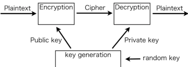
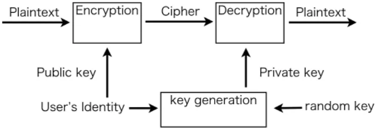
In 1984, A. Shamir proposed a new type of cryptographic scheme which is called the identity based encryption (IBE) [46]. The IBE scheme uses the identity of the user (e.g. user’s e-mail address) for the encryption (See Figure 4.2).
Figure 4.1: Public key cryptosystem
Cipher Plaintext Plaintext Encryption Decryption random key key generation
Figure 4.2: Identity-based cryptosystem Cipher Plaintext Plaintext Encryption Decryption random key key generation
Public key Private key
User s Identity
The pairing based cryptography is a new public key cryptographic scheme which was proposed after 2000 by three important works due to Joux [31], Sakai, Ohgishi and Kasahara [42] and Boneh and Franklin [8]. In these last two papers, the authors constructed an IBE scheme by using the Weil pairing on elliptic curves.
Scheme 1. IBE system using a bilinear map (BasicIdent) [8]
Let k be a positive integer and G1,G2 groups of order q, and e be a bilinear map e :G1× G1 → G2. Choose a random generator P ∈ G1. Choose a random element
s∈ F∗q and set P0 = sP . Choose hash functions H1 :{0, 1}∗ → G1 and H2 : G2 →
{0, 1}n.
We setP = {0, 1}n, C = G∗
1×{0, 1}n andK = {(q, G1,G2, e, n, P, P0, H1, H2)}. The
element s∈ F∗q is a master key.
For a given string ID ∈ {0, 1}∗, we set QID = H1(ID) ∈ G1 and the private key
RID= sQID.
For K = (q,G1,G2, e, n, P, P0, H1, H2), M ∈ P and a random element m ∈ Z∗q
eK(M ) = (mP, M + H2(gmID))
where gID = e(QID, P0).
dK(U, V ) = V + H2(e(RID, U )).
Boneh and Franklin give the setting of parameters for the IBE system based on the Weil pairing as follows: Let p be a prime p≡ 2 (mod 3) and N a positive integer such that p̸≡ 1 (mod N) and p2 ≡ 1 (mod N). The group G1 is the group of order
N of the group of points on the curve E : y2 = x3+ 1 over F
p, and G2 = µN is the
4.2
Pairing-friendly elliptic curves
Here we recall a pairing based cryptosystem using an elliptic curve over a finite prime field. Let p be a prime, K := Fp a finite field with p elements and E an
elliptic curve defined over K.
For a positive integer ℓ coprime to the characteristic of K, the Weil pairing is a map
eℓ : E[ℓ]× E[ℓ] → µℓ ⊂ ˆK∗
where ˆK is the field extension of K generated by coordinates of all points in E[ℓ],
ˆ
K∗ is the multiplicative group of ˆK and µℓ is the group of ℓ-th roots of unity in ˆK∗.
See Sections 3.4 and 3.5 for the details of the Weil pairing. The key idea of pairing based cryptography is based on the fact that the subgroup G = 〈P 〉 is embedded into the multiplicative group µℓ ⊂ ˆK∗ via the Weil pairing or some other pairing
map. Note that the smallest extension degree of the field extension ˆK/K is called
the embedding degree of E with respect to ℓ. It is known that E has the embedding degree k with respect to ℓ if and only if k is the smallest integer such that ℓ divides
pk− 1.
In pairing based cryptography, the following conditions must be satisfied to make a system secure:
• the order ℓ of a prime order subgroup of E(K) should be large enough so that
solving a discrete logarithm problem on the group is computationally infeasible and
• pk should be large enough so that solving a discrete logarithm problem on the
multiplicative group F∗pk is computationally infeasible.
Moreover for an efficient implementation of a pairing based cryptosystem, the fol-lowings are important:
• the embedding degree k should be appropriately small and • the ratio ρ = log p/ log ℓ should be appropriately small.
Elliptic curves satisfying the above four conditions are called “pairing-friendly” el-liptic curves.
In practice, it is currently recommended that ℓ should be larger than 2160 and
4.3
Construction of pairing-friendly elliptic curves
In this section, we summarize known results to construct pairing-friendly non-supersingular (i.e., ordinary) elliptic curves. First we show the conditions to con-struct pairing-friendly elliptic curves with embedding degree k with respect to ℓ.
Condition 1. 1. p, ℓ are primes and D is a square-free positive integer, 2. −D ≡ 0, 1 (mod 4)
3. k|(ℓ − 1), 4. 4p = t2+ Ds2,
5. #E(Fp) = p + 1− t ≡ 0 (mod ℓ),
6. Φk(p)≡ 0 (mod ℓ),
where Φk(x) is the k-th cyclotomic polynomial. The condition Φk(p) ≡ 0 (mod ℓ)
indicates that p has order k modulo ℓ. If we get integers p, ℓ, D, t, then we can construct elliptic curves satisfying the above condition by using the complex multi-plication method (CM method). The CM method is a construction method of the elliptic curve with prescribed order. The outline of the CM method is as follows: For a prime p ≥ 5 and a positive integer D such that 4p = t2 + Ds2 and −D ≡ 0, 1 mod 4,
1. compute the class polynomial HD[j](X) for the j-invariant function,
2. compute the reduction HD[j](X) mod p, calculate its roots ¯j,
3. let c = ¯j/(1728− ¯j), and E/Fp : y2 = x3+ 3cx + 2c.
Then E/Fp or its quadratic twist has the order p + 1−t. There are the CM methods
using the Weber function or other class invariants. Refer to [30] for the details of the calculation.
In [39], Miyaji, Nakabayashi and Takano give how to generate pairing-friendly curves with small embedding degree k = 3, 4, 6. The detail of their result is as follows.
Theorem 1 (Theorem 2, 3 and 4 in [39]). Let E be an ordinary elliptic curve over
Fq such that ℓ = #E(Fq) = q + 1− t is prime. Then the following table lists all the
Table 4.1: The MNT curves
k q t ℓ
3 12x2− 1 −1 ± 6x 12x2∓ 6x + 1 4 x2+ x + 1 −x or x + 1 x2+ 2x + 2 or x2+ 1 6 4x2+ 1 2x± 1 4x2∓ 2x + 1
Miyaji, Nakabayashi and Takano give a complete list for embedding degree k = 3, 4, 6. Furthermore we can estimate the ρ-value of this construction at 1, since the polynomials represent ℓ and p have degree two.
The study on the construction of pairing-friendly curves becomes an active area after the work by Miyaji, Nakabayashi and Takano. Another construction method is given by Cocks and Pinch [13] which can generate pairing-friendly elliptic curves with arbitrary embedding degree k.
Algorithm 9. Cocks-Pinch method
Input : k, ℓ, D ≡ 0 (mod 4) such that ℓ is a prime, −D is a square modulo ℓ and
k divides (ℓ− 1).
Output : p and t such that there is a curve with CM by D overFp with #E(Fp) =
p + 1− t where ℓ|(p + 1 − t) and ℓ|(pk− 1).
1. Choose a primitive k-th root of unity ζk∈ Fℓ.
2. Choose a∈ Z such that a ≡ 2−1(ζk+ 1) (mod ℓ).
3. If gcd(a, D)̸= 1, then return Step 1.
4. Choose an integer b≡ ±(a − 1)/√−D (mod ℓ) 5. Search j ∈ Z such that p = a2+ D(b + jℓ)2 is prime.
6. t← 2a.
7. Return p and t.
Since p = a2+ D(b + jℓ)2, we can estimate p = O(ℓ2). Therefore the value of ρ is approximately 2.
It becomes an open problem how to construct pairing-friendly elliptic curves such that the value of ρ is 1 for the prescribed embedding degree k.
Freeman gives the construction with embedding degree 10 in [21].
t(x), ℓ(x), and q(x) by
ℓ(x) = 25x4+ 25x3+ 15x2+ 5x + 1,
t(x) = 10x2+ 5x + 3,
q(x) = 25x4+ 25x3+ 25x2+ 10x + 3.
If the equation u2− 15Dv2 =−20 has a solution with u ≡ 5 (mod 15), then (t, q, ℓ)
represents a family of curves with embedding degree 10.
Barreto and Naehrig [2] give a family that (t, ℓ, q) parametrizes a family of pairing-friendly elliptic curves with embedding degree 12 and the discriminant D = 3.
Example 2 ([2]). Let
ℓ(x) = 36x4+ 36x3+ 18x2+ 6x + 1,
t(x) = 6x2+ 1,
q(x) = 36x4+ 36x3+ 24x2+ 6x + 1.
Then (t, q, ℓ) represents a family of curves with embedding degree k = 12.
This family is a complete family for k = 12 and ρ≈ 1.
We recall the construction by Brezing and Weng, called the BW method. We describe their main idea. For an embedding degree k and a discriminant D > 0, consider the number field M ∼=Q(ζk,
√
−D). Suppose M ∼=Q[x]/(f(x)). Note that deg f (x) = ϕ(k) if √−D ∈ Q(ζk) and deg f (x) = 2ϕ(k) if
√
−D ̸∈ Q(ζk), where
ϕ is the Euler’s phi function. We can compute a polynomial g(x) and h(x)∈ Z[x]
which represent ζk and
√
−D, respectively. We set a(x) = (g(x) + 1) and b(x) =
(a(x)− 2)h(x) ∈ Q[x]/(f(x)). We test if there exists some integer x0 such that
b(x0)≡ 0 mod D. We define
p(x) = 1
4(a(x)
2+ b(x)2/D). Now suppose the following conditions are satisfied:
1. p(x) is irreducible.
2. p(x) has integer values for x0 mod D and 3. f (−Dy + x0)∈ Z is irreducible.
We can now try to find primes ℓ = f (x1) for some x1 ≡ x0 mod D and test whether
p(x1) is prime as well. Brezing and Weng gave some examples in their paper. Freeman, Scott and Teske give the best ρ-values for family of pairing-friendly curves with embedding degree k ≤ 50. We show the currently best ρ-values for pairing-friendly elliptic curves with embedding degree k≤ 50 in Table 4.2.
Table 4.2: k, ρ-value, discriminant D and the degree of ℓ(x) obtained by the Free-man, Scott and Teske method
k ρ D deg ℓ(x) k ρ D deg ℓ(x) 14 1.333 3 12 28 1.333 1 12 16 1.250 1 8 30 1.500 3 8 18 1.333 3 6 32 1.063 3 32 20 1.375 3 16 34 1.125 3 32 22 1.300 1 20 36 1.167 3 24 24 1.25 3 8 38 1.111 3 36 26 1.167 3 24 40 1.375 1 16
Freeman, Scott and Teske give the construction for various D̸= 1, 3.
In [24], they list bit sizes matching the security levels of the the SKIPJACK, Triple-DES, AES-Small, AES-Medium, and AES-Large symmetric key encryption schemes. To achieve the levels of security for a system with an elliptic curve of the subgroup size 160 bit and the extension field size 1280 bit, curves with the embedding degree 8 are recommended for ρ≈ 1 from Table 4.3.
Table 4.3: Bit sizes of curve parameters and corresponding embedding degrees to obtain commonly desired levels of security.([24])
Security level Subgroup size Extension field size Embedding degree
(bit) ℓ (bit) qk (bit) ρ≈ 1 ρ≈ 2
80 160 960 - 1280 6 - 8 2,3 - 4
112 224 2200 - 3600 10 - 16 5 - 8
128 256 3000 - 5000 12 - 20 6 - 10
192 384 8000 - 10000 20 - 26 10 - 13
4.4
Constructing pairing friendly elliptic curves
for the embedding degree 2n, n is odd prime
Here we recall the framework of generating pairing-friendly elliptic curves for a given
k using the CM method.
Step 1 : Find integers ℓ, q, a, b, and D(> 0) satisfying the following conditions: 1. 4q− a2 = Db2,
2. q + 1− a ≡ 0 (mod ℓ),
3. k is the smallest positive integer such that qk− 1 ≡ 0 (mod ℓ). 4. q and ℓ are primes.
5. −D ≡ 0 or 1 (mod 4)
Step 2 : Using the CM method, find an elliptic curve E/Fq such that
1. #E(Fq) = q + 1− a.
2. E has complex multiplication by an order in Q(√−D)
Note that conditions 2 and 3 in Step 1 yield a− 1 is a primitive k-th root of unity inFℓ.
4.5
Our construction
We only consider the case that q = p is prime and k is of the form k = 2n where n is odd.
First note that for k = 2n with odd n, if g is a primitive k-th root of unity in a field K, then √−g = g(n+1)/2 belongs to K. Our idea is to use this√−g = g(n+1)/2 as √−D. The advantage to use such √−D is that we do not need to extend a cyclotomic fieldQ(ζk) to obtain a small value of ρ = log p/ log ℓ.
Our method based on this idea is divided into two cases. In the following, we describe our method.
Let g be a positive integer such that ℓ := Φk(g) is a prime number. Then, g is
a primitive k-th root of unity modulo ℓ and √−g ≡ g(n+1)/2 (mod ℓ). Take D, a, b (0 < D, a, b < ℓ) as follows:
D := g, a := g + 1,
Then, p = (a2 + Db2)/4 = O(gn+2) and ℓ = O(gϕ(n)), where ϕ denotes the Euler’s phi function.
In this case, we have ρ≈ (n + 2)/ϕ(n) as p, ℓ → ∞. In particular, if n is a prime number, we obtain ρ≈ (n + 2)/(n − 1).
Remark: The above method works well in most cases but there are some
unfortu-nate cases. When k = 30, a2+ Db2 in the above has no chance to be divisible by 4. Taking b as b = (g− 1)g(n−1)/2= g8− g7 without taking modulo ℓ, we can make
a2+ Db2 divisible by 4, but it makes ρ greater than 2. When n≡ 1 (mod 4), we can improve the value of ρ.
Let g be a positive integer such that ℓ := Φk(g) is a prime number. Then, g is a
primitive k-th root of unity under modulo ℓ and√−g ≡ g(n+1)/2 (mod ℓ). Note that
g(n+1)/2is also a primitive k-th root of unity modulo ℓ. Take D, a, b (0 < D, a, b < ℓ) as follows: D := g, a := g(n+1)/2+ 1, b :≡ (g(n+1)/2− 1)g(n+1)/2/g (mod ℓ). Then, since b ≡ (g(n+1)/2− 1)g(n−1)/2≡ gn− g(n−1)/2 (mod ℓ) ≡ −1 − g(n−1)/2 (mod ℓ),
p = (a2+ Db2)/4 = O(gn+1) and ℓ = O(gϕ(n)).
Hence, in this case, we have ρ≈ (n + 1)/ϕ(n) as p, ℓ → ∞. In particular, if n is a prime number, we obtain ρ≈ (n + 1)/(n − 1).
4.6
Table of ρ-values (as p, ℓ
→ ∞)
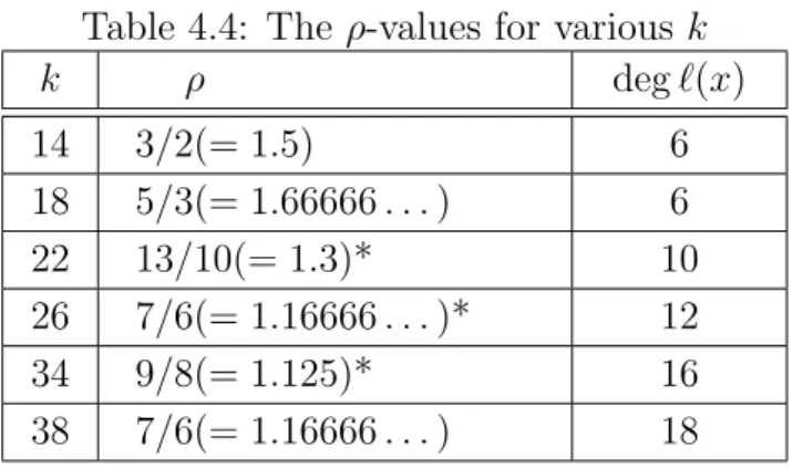
We show the table of values of ρ obtained by our method for k = 2n with odd n, 6 < n < 20 but n̸= 15.
In Table 4.4, the symbol * means that the ratio is the same value achieved by [24]. We emphasis that our result is obtained without extending a cyclotomic field Q(ζk), whereas in [24] the case k = 2n with odd n needs a field extension. Hence in
the above cases, we achieve the same value of ρ as in Freeman-Scott-Teske’s result [24], but with smaller q and ℓ than ones in [24].
Since the degree of ℓ(x) in our method is smaller than in Freeman-Scott-Teske’s method, it is expected that one can obtain sufficiently many pairing-friendly elliptic curves of order about 2160 for the embedding degree k = 2n. In practice, one can
Table 4.4: The ρ-values for various k k ρ deg ℓ(x) 14 3/2(= 1.5) 6 18 5/3(= 1.66666 . . . ) 6 22 13/10(= 1.3)* 10 26 7/6(= 1.16666 . . . )* 12 34 9/8(= 1.125)* 16 38 7/6(= 1.16666 . . . ) 18
obtain smaller primes ℓ by using our method than using the Freeman-Scott-Teske method; see Tables 4.5 and 4.6. These tables show that our method can produce more pairing-friendly elliptic curves than the Freeman-Scott-Teske method does.
Table 4.5: The smallest three primes ℓ obtained by using our method
k log ℓ 14 23.3 26.2 44.3 22 92.8 107.0 122.1 26 54.2 135.8 145.7 34 182.7 225.4 228.3 38 189.6 213.6 230.6
Table 4.6: The smallest three primes ℓ by using the Freeman-Scott-Teske method [24] k log ℓ 14 70.3 123.1 123.3 22 92.8 206.5 250.7 26 349.3 350.2 354.5 34 442.7 447.4 472.2 38 284.2 357.9 369.8
Chapter 5
Pairing-friendly elliptic curves
with small security loss by
Cheon’s algorithm
Some pairing-based encryption schemes are proposed their security based on the hardness of the q-weak/strong Diffie-Hellman problem. The Cheon’s algorithm [11] is an attack to calculate effectively the q-weak/strong Diffie-Hellman problems. We consider the effect of the Cheon’s algorithm for some methods to construct pairing-friendly elliptic curves.
5.1
Pairing-related problems
In 2002, Mitsunari, Sakai and Kasahara proposed a traitor tracing scheme based on the q-weak Diffie-Hellman problem [38]. The definition of the q-weak Diffie-Hellman problem is as follows.
Definition 6 (The q-weak Diffie-Hellman problem). Let G be an abelian group
whose order is a large prime number ℓ. The q-weak Diffie-Hellman problem asks
[1/α]g for a (q + 1)-tuple (g, [α]g, [α2]g, . . . , [αq]g) where g∈ G and α ∈ (Z/ℓZ)∗.
The q-weak Diffie-Hellman problem is also called the “q-Diffie-Hellman inversion problem” in [5].
In 2004, Boneh and Boyen proposed a short signature scheme based on the q-strong Diffie-Hellman problem which is defined as follows [6].
Definition 7 (The q-strong Diffie-Hellman problem). Let G be an abelian group
a pair ([1/(α + a)]h, a) where a is any element in (Z/ℓZ)∗ for a (q + 2)-tuple (h∈ H, g, [α]g, [α2]g, . . . , [αq]g) where H is an abelian group of order ℓ, g ∈ G and
α∈ (Z/pZ)∗.
After Mitsunari, Sakai and Kasahara’s work [38] and Boneh and Boyen’s work [6], many protocols without random oracles have been proposed based on weak Diffie-Hellman-like problems, e.g. [5], [7], [41]. In the following, we call such kind of problems the “pairing-related problems”.
For the definitions of other pairing-related problems, e.g. the q-bilinear Diffie-Hellman inversion problem and the (q+1)-bilinear Diffie-Diffie-Hellman exponent problem, see [5], [7] and so on.
5.2
Cheon’s algorithm and its improvement
In Eurocrypt 2006, Cheon [11] proposed an algorithm to solve the q-weak/strong Diffie-Hellman problem. In Pairing 2007 Kozaki, Kutsuma and Matsuo [34] im-proved the complexity of Cheon’s algorithm for the q-weak Diffie-Hellman problem. For an abelian group G of prime order ℓ, if ℓ− 1 has a positive divisor d less than or equal to q, then their improved algorithm can solve the q-weak Diffie-Hellman prob-lem within O(√ℓ/d +√d
)
group operations using space for O (
max(√ℓ/d,√d
)) group elements. There also exists an ℓ + 1 variant of this algorithm. The Cheon’s original algorithm in [11] is as follows:
Algorithm 10. Cheon’s algorithm
Input : Let G be an abelian group of prime order p, g, g1, gd ∈ G and d be a
positive integer such that d|(ℓ − 1).
Output : α∈ F∗p such that g1 = [α]g and gd= [αd]g.
1. Find a generator ζ0 ∈ F∗ℓ.
2. ζ ← ζ0d. 3. d1 ← ⌈
√
(ℓ− 1)⌉.
4. Find u1, v1 such that 0 ≤ u1, v1 < d1 and [ζ−u1]gd = [ζd1v1]g by the baby
step/giant step method. 5. k0 ← d1v1+ u1.
6. d2 ← ⌈
√ d⌉.
7. Find 0 ≤ u2, v2 ≤ d2 such that [ζ−u
2(p−1)/d
0 ]g1 = [ζ
k0+d2v2(p−1)/d
0 ]g by the baby
step/giant step method. 8. Return ζk0+(d2v2+u2)(ℓ−1)/d
0 .
Theorem 2 ([34]). Let g be an element of prime order ℓ in an abelian group.
Sup-pose that d is a positive divisor of ℓ−1. If g, [α]g and [αd]g are given, α can be
com-puted within O(√ℓ/d +√d
)
group operations using space for O
(
max(√ℓ/d,√d
))
group elements.
Theorem 3 ([34]). Let g be an element of prime order ℓ in an abelian group.
Suppose that d is a positive divisor of ℓ + 1 and [αi]g for i = 1, 2, . . . , 2d are given.
Then α can be computed within O(√ℓ/d + d
)
group operations using space for O
(
max(√ℓ/d,√d
))
group elements.
Remark 1. In the original result of Cheon [11], the complexity in the above two
theorems were given by O
( log ℓ(√ℓ/d +√d )) and O ( log ℓ(√ℓ/d + d )) group operations, respectively.
5.3
The Effect of Cheon’s algorithm for
construct-ing pairconstruct-ing-friendly elliptic curves
In this section, we consider the effect of Cheon’s algorithm on known methods for constructing pairing-friendly elliptic curves.
With respect to Cocks-Pinch method, the group size ℓ can be randomly chosen. So it is not difficult to avoid the security loss by Cheon’s algorithm. See Section 6 of [34] for the details.
Except for Cocks-Pinch method, since the group order ℓ is given by a polynomial
ℓ(x), we should be careful about the effect of Cheon’s algorithm. Roughly speaking,
if ℓ± 1 has a factor d, the cost for solving the q-strong Diffie-Hellman problem is reduced by a factor √d. So, if a polynomial ℓ(x) ± 1 is reducible and its
non-trivial polynomial factor h(x) has a small degree, there is at least a (log h(x0))/2 bit security loss by Cheon’s algorithm when we take ℓ = ℓ(x0) for an integer x0. In the following, we see the security loss by Cheon’s algorithm for each method using polynomials.
The MNT method and its variant.
In the MNT method based on Miyaji, Nakabayashi and Takano’s result [39], the following polynomials are used: ℓ(x) = 12x2± 6x + 1 for k = 3, ℓ(x) = x2+ 2x + 2
or x2+ 1 for k = 4 and ℓ(x) = 4x2± 2x + 1 for k = 6. Except for ℓ(x) = ℓ2+ 2ℓ + 2 in the case k = 4, ℓ(x)− 1 is divisible by x. For the generalized MNT method such as Galbraith, McKee and Valen¸ca’s method [28], there are some cases that ℓ(x)± 1 are reducible. Since the degree of ℓ(x) equals two, this fact does not lead directly that Cheon’s algorithm affects the security of each curve.
Cyclotomic Families
There are some methods using a cyclotomic polynomial as ℓ(x), e.g. Brezing and Weng’s method [9] and Freeman, Scott and Teske’s method [24]. We call a family of pairing-friendly curves obtained by these methods a ”cyclotomic family”. The advantage of a cyclotomic family is that one can take curves with relatively small
ρ = log ℓ/ log p (< 2).
All of them use a cyclotomic polynomial to set a prime ℓ as ℓ = Φk(x) or
ℓ = Φck(x) for some c > 1 where k is the embedding degree. Then, ℓ− 1 is factored
by x at least. Moreover, if ck = 2m, then ℓ−1 is factored by x2m−1, otherwise ℓ−1 is factored by x(x+1) or x(x−1). The size of x is about (log ℓ)/ϕ(ck) bit, c ≥ 1, where
ϕ is the Euler’s phi function. Hence, if x < q (resp. x(x + 1) < q), the complexity
to solve the q-weak Diffie-Hellman problem is reduced to O(√ℓ1−1/ϕ(ck)+√ℓ1/ϕ(ck)) (resp. O(√ℓ1−2/ϕ(ck)+√ℓ2/ϕ(ck))) group operations.
Other methods.
For k = 10, Freeman gave the following family [20].
p(x) = 25x4+ 25x3+ 25x2+ 10x + 3
ℓ(x) = 25x4+ 25x3+ 15x2+ 5x + 1
Dy2 = 15x2+ 10x + 3 For this family, ℓ(x)± 1 factor as
ℓ(x)− 1 = 5x(5x3+ 5x2+ 3xz + 1)
ℓ(x) + 1 = (5x2+ 1)(5x2+ 5x + 2). The following two examples are given in [20].
ℓ = 503189899097385532598571084778608176410973351
The former is a 149 bit prime and the latter is a 196 bit prime. For each example,
ℓ− 1 factors as
ℓ− 1 = 2 · 52· 853 · (a 33 bit prime) · (a 39 bit prime) · (a 63 bit prime) ℓ− 1 = 22· 52· 7 · (a 29 bit prime) · (a 44 bit prime) · (a 114 bit prime)
respectively. Cheon’s algorithm affects each case.
For k = 12, Barreto and Naehrig gave the following family [2].
ℓ(x) = 36x4+ 36x3+ 18x2+ 6x + 1
p(x) = 36x4+ 36x3+ 24x2+ 6x + 1
Dy2 = 3(6x2+ 4x + 1) For this family, ℓ(x)± 1 factor as
ℓ(x)− 1 = x(6x3+ 6x2+ 3x + 1)
ℓ(x) + 1 = (3x2+ 3x + 1)(6x2+ 1). The following example is given in [2].
ℓ = 1461501624496790265145447380994971188499300027613 (160 bit)
For this example, we have
ℓ− 1 =22· 3 · (a 24 bit prime) · (a 38 bit prime) · (a 39 bit prime) · (a 57 bit prime)
ℓ + 1 =2· 7 · 13 · 19 · 1279 · 1861 · 21227 · (a 19 bit prime) · (a 21 bit prime) · (a 24 bit prime) · (a 50 bit prime).
Hence Cheon’s algorithm affects the security of this example.
5.4
How to reduce a security loss of a cyclotomic
family
In this section, we consider the way to reduce the security loss by Cheon’s algorithm for a cyclotomic family with embedding degree 2n where n is an odd prime. As we see in the previous section, a cyclotomic family uses the ck-th cyclotomic polynomial Φck(x) as ℓ = ℓ(x) for finding a pairing-friendly elliptic curve of an embedding degree
algorithm, we propose to take a prime ℓ as a large proper divisor of Φk(x) for an
integer x.
In a cyclotomic family, the best ρ-value for each embedding degree k = 2n for an odd prime n is given by the Freeman-Scott-Teske method. However, since the Freeman-Scott-Teske method uses Φck(x) for c≥ 2, it is difficult to find a suitable
order ℓ only by taking a proper divisor of Φck(x). We give the search result using
the Freeman-Scott-Teske method in Table 5.1. In this search, for each k we used D and Φck(x) as shown in [24] which gave the best ρ-value and searched ℓ satisfying
the following condition:
• Φck(x) = ℓ· (a positive integer less than 10000)
• ℓ ± 1 = (a positive integer < 210)· (a product of primes ≥ 250).
Table 5.1: The size of the smallest ℓ(≤ 2400) satisfying the condition
k the size of ℓ 14 180 bit 22 338 bit 26 Not found 34 Not found 38 Not found
As Table 5.1 shows, it is difficult to find a suitable ℓ of appropriate size except for
k = 14. It is mainly because the degree of Φck(x) is relatively large for c ≥ 2. So it is
important to use Φk(x) to search a pairing-friendly elliptic curve of the embedding
degree k which is not affected by Cheon’s algorithm. In the following section, we propose an improved method for the embedding degree 2n where n is an odd prime and we show the efficiency of the proposed method by giving the experimental data.
5.5
The condition of a large prime factor of Φ
2n(x)
First, we study the condition for the large prime factor ℓ of Φ2n(x). Note that when
n is an odd prime, Φ2n(x) = Φn(−x).
Lemma 1. Let n and ℓ be primes and x an integer. If Φn(x) ≡ 0 (mod ℓ), then
Proof. Assume that Φn(x) ≡ 0 (mod ℓ) and ℓ ̸= n. Then Φn(x) ≡ 0 (mod ℓ)
yields that x gives a primitive n-th root of unity in (Z/ℓZ)∗. Hence n divides #(Z/ℓZ)∗ = ℓ− 1; that is, ℓ ≡ 1 (mod n).
Theorem 4. Let k be a positive integer of the form k = 2n, where n is an odd
prime. Let x be an integer, ℓ a large prime greater than n and s a small integer such that Φk(x) = sℓ. Then the following holds:
1. If s is divisible by n, then x≡ −1 (mod n) and s is not divisible by n2. 2. If s = n, then ℓ− 1 is divisible by x + 1.
3. If s is not divisible by n, then x̸≡ −1 (mod n).
Remark 2. In Theorem 4, note that by the assumption ℓ > n and Lemma 1, ℓ− 1
is divisible by n. Moreover, it is easy to see that ℓ2 − 1 is divisible by 24. Hence (ℓ + 1)(ℓ− 1) is divisible by 24n. We also note that if s is a small prime which
divides Φ2n(x) for an integer x, then s = n or s ≡ 1 mod n.
Proof. First, note that ℓ− 1 = Φk(x)/s− 1 = (Φn(−x) − s) /s. Second, note that if
x̸≡ −1, then Φk(x) = Φn(−x) = ((−x)n− 1) /(−x − 1) ≡ (−x − 1)/(−x − 1) = 1
(mod n) and hence, if n divides s, we have x≡ −1 (mod n).
(1) From the above, if n divides s, then x≡ −1 (mod n). Hence, we only have to show that n2 does not divide s. Write s = tn where t is an integer. Since ℓ ≡ 1 (mod n) from the assumption of the theorem and Φn(−x) − tn = Φk(x)− tn =
tn(ℓ− 1), we have that Φn(−x) − tn ≡ 0 (mod n2). Since Φn(−x) ≡ n (mod n2) in
this case, we have that t̸≡ 0 (mod n); that is, n2 does not divide s.
(2) If s = n, then since Φk(−1) − s = Φn(1)− n = 0, Φk(x)− s has a factor
x + 1. More precisely, we have Φk(x)− n = Φn(−x) − n = −(x + 1)((−x)n−2 +
2(−x)n−3+· · · + (n − 2)x + (n − 1)). Since x + 1 ≡ 0 (mod n) in this case and n is
an odd prime, (−x)n−2+ 2(−x)n−3+· · · + (n − 2)(−x) + (n − 1) ≡ n(n − 1)/2 ≡ 0
(mod n). Hence, we have ℓ− 1 = (Φn(−x) − n)/n has a factor x + 1.
(3) Suppose that x ≡ −1 (mod n). Then Φk(x) ≡ Φn(1) ≡ 0 (mod n). This
contradicts the assumption that n does not divide s.
In particular, the case (2) in Theorem 4 is not suitable for the protocols based on pairing-related problems if we consider an effect of Cheon’s algorithm.
5.6
Our result
From the result of the previous section, we propose a method to construct pairing-friendly elliptic curves with small security loss by Cheon’s algorithm.
We consider only the case that the embedding degree k is in the form k = 2n where n is an odd prime. Our construction given in Section 4.5 is an improved version of the Freeman-Scott-Teske method. Since the Freeman-Scott-Teske method needs a field extension, we should use Φck(x) where c is an extension degree. So when we
take ℓ as a proper divisor of a cyclotomic polynomial in the Freeman-Scott-Teske method, ℓ and p become much larger. Here, we improve the Freeman-Scott-Teske method such that we can obtain the small ρ value with not so much large ℓ and p even when we take ℓ as a proper divisor of a cyclotomic polynomial.
We give the algorithm with small security loss by Cheon’s attack based on our construction in Section 4.5.
Algorithm 11. Curve construction with small security loss by Cheon’s algorithm Input : n: an odd prime; α, β, q: positive integers
Output : p, ℓ : primes, E/Fp : an elliptic curve over Fp such that #E(Fp) ≡ 0
(mod ℓ) and its embedding degree equals k = 2n.
1. Find g∈ Z>0 such that Φk(g) = sℓ where ℓ is a large prime, s is a small prime
(̸= n) or n·(a small prime) and
ℓ− 1 = 2n(a positive integer ≤ 2α)∏(prime≥ q)
ℓ + 1 = 2(a positive integer ≤ 2β)∏(prime≥ q)
2. Set a := g + 1 if n≡ 3 (mod 4) and a := g(n+1)/2+ 1 if n≡ 1 (mod 4). Take b
as a positive integer (< ℓ) such that b≡ (a−2)g(n+1)/2/g (mod ℓ). Set D := g and check whether p := (a2+ Db2)/4 is prime or not. If not, return to Step 1.
3. Use the CM method and output the result.
The positive integer q in the input is a parameter of the q-weak/strong Diffie-Hellman problem. The size of q depends on a protocol and the ability of attackers. The positive integers α and β in the input are parameters which determine the bound of the security loss by Cheon’s algorithm. We take α = β = 6 for examples in the next section.
In general, it is hard to construct the elliptic curve by the CM method for a large
D. Therefore we must be careful with the size of D.
In our method, we set D = g. If g is not square free, then we set the square free part of g as D. So the size of g is important when we construct the elliptic curve using the CM method. But as stated in [24], we can construct an elliptic curve by using the CM method for D < 1010. Hence our method is effective to construct pairing-friendly elliptic curves.
5.7
Examples
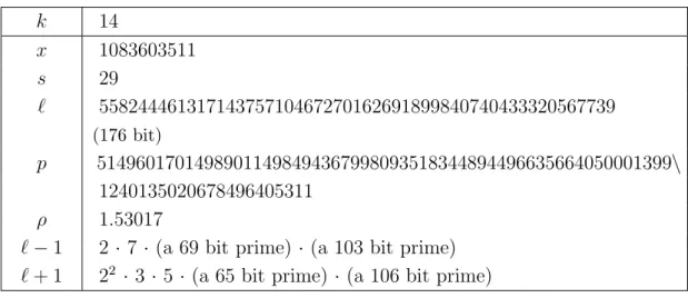
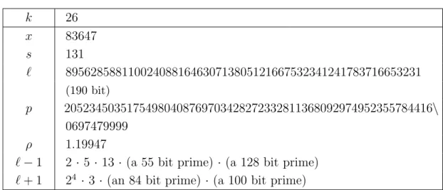
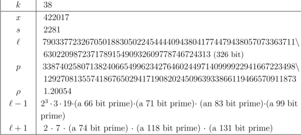
Here we show examples of pairing-friendly elliptic curves with small security loss by Cheon’s algorithm. The following examples are obtained by using Algorithm 11 with q = 250 and α = β = 6 for 14 ≤ k ≤ 38. The security loss of these examples is within 5 bit, if the parameter q in the weak/strong Diffie-Hellman problem is less than 50 bit. If the parameter q is about 260, we can find examples for q = 260 by taking α = β = 11. See from Table 5.2 to 5.6.
Table 5.2: The curve obtained by using Algorithm 11 for k = 14
k 14 x 1083603511 s 29 ℓ 55824446131714375710467270162691899840740433320567739 (176 bit) p 51496017014989011498494367998093518344894496635664050001399\ 1240135020678496405311 ρ 1.53017
ℓ− 1 2 · 7 · (a 69 bit prime) · (a 103 bit prime)
ℓ + 1 22 · 3 · 5 · (a 65 bit prime) · (a 106 bit prime)
Table 5.3: the curve obtained by using Algorithm 11 for k = 22
k 22 x 2169245 s 67 ℓ 34435869083893646715039335514954459125462349808949323158099\ 743 (205 bit) p 58877786517045158480579461956011716339017570871437492980201\ 25450311726006289864629 ρ 1.32879
ℓ− 1 2 · 11 · (a 74 bit prime) ·(a 127 bit prime)
Table 5.4: the curve obtained by using Algorithm 11 for k = 26 k 26 x 83647 s 131 ℓ 895628588110024088164630713805121667532341241783716653231 (190 bit) p 20523450351754980408769703428272332811368092974952355784416\ 0697479999 ρ 1.19947
ℓ− 1 2 · 5 · 13 · (a 55 bit prime) · (a 128 bit prime)
ℓ + 1 24 · 3 · (an 84 bit prime) · (a 100 bit prime)
Table 5.5: the curve obtained by using Algorithm 11 for k = 34
k 34 x 1730735 s 17· 137 ℓ 27830402151707213772790243425060710128851524965270716441651\ 11328554663063808567192444024844854329 (321 bit) p 48538978648626809809653096381338491065159598631595616079566\ 88321815318124568522625897243485762842754461264104559 ρ 1.15803
ℓ− 1 23 · 17 · (a 92 bit prime) · (a 222 bit prime)
Table 5.6: the curve obtained by using Algorithm 11 for k = 38 k 38 x 422017 s 2281 ℓ 79033772326705018830502245444409438041774479438057073363711\ 630220987237178915490932609778746724313(326 bit) p 33874025807138240665499623427646024497140999922941667223498\ 12927081355741867650294171908202450963933866119466570911873 ρ 1.20054
ℓ− 1 23· 3 · 19·(a 66 bit prime)·(a 71 bit prime)· (an 83 bit prime)·(a 99 bit prime)
![Table 4.3: Bit sizes of curve parameters and corresponding embedding degrees to obtain commonly desired levels of security.([24])](https://thumb-ap.123doks.com/thumbv2/123deta/8513267.1805666/26.892.198.741.884.1054/table-parameters-corresponding-embedding-degrees-commonly-desired-security.webp)