Stochastic Mean-Variance Optimization in
Portfolio Analysis
著者名(英)
Midori Munechika
journal or
publication title
The economic review of Toyo University
volume
31
number
1
page range
1-21
year
2005-12
URL
http://id.nii.ac.jp/1060/00001685/
Creative Commons : 表示 - 非営利 - 改変禁止
東洋大学「経済論集」
31巻1号2005年12月
Stochastic Mean−Variance Optimization
in Portfolio Analysis
Midori Munechika’
−︵∠﹁54.56
Contents Introduction Matrix Approach to Portfolio Risk Mean−Variance Optimization Problem Stochastic Optimization by Monte Carlo Simulation Stylized Facts about Return Distributions Concluding Remarks and Future Direction of Research1.Introduction
The Markowitz mean−variance analysis that Iaid the foundations of modem portfolio theory (MPT)shows how rational investors should construct their optimal portfolios under conditions of uncertainty. Why is his theory called mean−variance analysis? It is because only two parameters, mean retum and return variance(or standard deviation), are taken into account to construct the optimal portfolio. Essentially, the aim of investors is to maximize the terminal value of their investment. The mean−variance apProach needs to justify the switch from maximization of utility of wealth to utility consisting of two characteristics:mean retum and retum variance. Theoretically, this can be done by making two hypotheses behind the theory:the normal distribution hypothesis about return distributions and a quadratic utility fUnction(see Munechika[2002]). Mean−variance analysis is clearly classified as a normative theory rather than a positive one, while it approaches nomative issues in a positive context. Sharpe[1963]summarizes the process of Markowitz’s portfolio selection into three steps:(1)making probabilistic estimates of 章Financial s山pport ftom Granトin・Aid fc)r Scientl丘c Research(C−No.15530227)of戊apan S㏄]et》. for the Prometion ofScience{戊SPS)under the Ministny’of Education、 Culture, Sports. Sclenc己and T㏄hnology(MEXT)and a grant frorn Toyo Universit}’ a[e gratefu1]}. acknowlcdgcd.the future perf()rmances ofasset retums,(2)analyzing those estimates to determine an efficient set ofportfolios, and(3)selecting from that set the portfolios best suited to the investor’s preferences. Corresponding to these three steps, a portfolio optimization methodology is composed ofthree key ingredients:aretum forecast, an optimizer(i.e., a software program used in the computational procedure)and a utility fUnction. The first step of the process(i.e., the normal distribution hypothesis)makes the Markowitz model into stochastic one. The major concem of this article is to introduce a method of stochastic optimization by applying Monte Carlo simulation to the second step and to examine its usefulness and its limitations. In Section 2, I define portf()lio return and risk by using matrix notation and point out that a covariance matrix is a concise fbrm fbr the in f()rmation of volatilities and correlations of assets and that is usefUl fbr constructing optimal portfblios. In Section 3, the mean−variance optimization problem is mathematically formulated and its solution is provided by quadratic programming. In Section 4, l implement the mean−variance optimization problem by using the method of Monte Carlo simulation. In Section 5, the stylized facts about return distributions are discussed in the context of stochastic optimization.
2.Matrix Approach to Portfolio Risk
I first formulate the problem of Markowitz‘s mean−variance optimization in a formal mathematical context. Suppose that a portfolio is composed of n risky assets. The retum on aportfolio is a weighted average of individual asset returns.R,一・・Vl・Rl+W、・R,+…+1’・.・’・Rn一ΣW,Rt (1)
’ニl n wh・・eΣw,−1・Th・・e・・m・n・h・i−・h・i・ky asse・i・R, and・h・p・rti・n・f・h・↓一・h asse・h・ld ’=l in the portfolio is w,. Portfolio risk is defined as portfblio returns variance.v・・ [R,]一σ; (・)
The variance ofthe portfblio return is the mixture of variability of returns fbr respective assets and their co−movement, which can be expressed in a matrix format as in the following table.Stochastic Mean−Variance Optimization in Portf()lio Analysis
Asset l Asset 2 .■■
Assetη
Assct 1 2 2@ σ1Wl
WIW2σ12
... Wlw。σ1“ Asset 2 W2}ylσ21 2 2W2σ2 ・㊨. W2Wησ2η ⋮ ⋮ ⋮ .. @. ⋮ Asset〃 wηw1σ“1 w。w2σ。2 ・.. 2 2w,1σ月 The diagonal terms contain the variances of the individual assets and the off−diagonal terrns contain the covariances. The covariance between retums on the i th asset and the/th asset is given by:C・・(ノ∼i ,Rノ)=E[(R,一μ、)(Rノーμノ)]=σt, (3)
where,tli andμノare the mean retums of R, and R.f respect・ively. The sign ofthe covariance will indicate the direction ofcovariance Ri and RゾThus, the variance of a portfolio’s retum can be calculated as the sum ofall the cells ofthe table. 】n2n tln
σ㌍w品・w錫+…+w編+ΣΣ・’iw,σi、+ΣΣ・v・・vノσ・、+…+ΣΣWniv」σnJ ’=1 ノ=1 ’=2 ノ=l i=n .ノ=1 ∫≠ノ i≠ノ i≠ノ n n n一Σw∼σ∼+ΣΣγσ, (4)
’=| ’=1 ノ=1 va「iance・term i≠ノ COVarianCe terrn In the double summation i≠ノof the covariance term, if l=ゾ, then the te㎜would be w,・w、a“・w、 ・’堰Ei・・eσ,,−E[(R,一μ、)(Ri一μ、)]−E(R,一μ,)2一σ,、. Thi・i・the exactly th・ variance term in the first summation. The portfolio risk can also be written as: n nσ; ・IE)Σw、W、σ, (5)
’ニ1ノ=l It is convenient to present the portfolio return and risk in the form of matrix notation as shown in the above explanation. The set of asset returns is expressed as a column vector consisting ofthe random variable R,,…,1∼n: = ヰ・Σ国
R...R
ノ
(6) The set of port fblio weights is:■
W
=W
・Σ国
ヱ
ア
W.:W
The retum on a portfblio ofequation(1)may be written as: n R,一Σw、R,一[WI RI…1’・。・Rn]一[w1…w,、 ハ=l where wT is a transpose of w: w7’・・[Wl…w。] The portfblio variance ofequation(5)is expressed as: 2 2 W1σ1 WlW2σ12 ”°σ;一ΣΣW、W、σij−W2㍗σ21 W’92 ::’
WηWlση1 WηW2σ〃2 ’”W
カ
R...R
T =W 「 WIWnσln W2 Wnσ2n … 2 2 wηση hich can be broken down into the following matrix multiplications: σ; 一[wl w2 … wη] り↑−烈゜: 川σσ σ
σ12 ’” 2 σり ’” σ〃2 ’■一 σln σ2n 2 σn w|W2
wη=wTVw
(7) (8) (9) (10) (11)where V is a variance−covarlance variance tems on the diagonal and the
covariance terms on the off−diagonal The variance−covariance matrix is also referred to as the covariance matrix. The covariance matrix V is always square and symmetric. In fact, the covarianceσu between risky asset i and risky asset/wiIl be equal to the covariance between risky asset / and risky asset i:σ,,=σ、, (12)
Then, V can be arranged in the following square matrix: σ1 σ12 ’” σln σ1 2V=σ21σ・’”σ・n=σ12
2 σnl σn2 ’” σn σln Therefbre, V is also symmetric. The covariance matrix demonstrates σ12 2 σ2 σ2n ’”@ σln ’”@ σ2n 2 ’”@ σn (13) how to reduce the portfblio risk through portfolioStochastic Mean−Variance Optimization in Portfc)lio Analysis diversification. As the number of assets n increases, the total number of elements in the
covariance matrix becomesη2,the number of variance tems becomes n,and the number of
・・va・i・nce t・m・th・・bec・m・・(〃2−〃). F・・ex・mpl・,・p・rtf・li・・f l OO・t・・k・h・・100 variance temis and 9900 covariance terms. It is clear that the risk ofa portfolio with many assets is more dependent on the covariances between the individual assets than on the variances of the individual assets. Therefbre, the degree of co−movements between different pairs of stocks in a portfblio is crucial to estimate and reduce the portfblio risk. There is another typical measure of the degree of co−movement between two variables: correlation. The magnitude of covariance,σ〃depends not only on the degree ofco−movement among the retums but also on their sizes. For instance, the covariance of monthly retums will normally be greater than the covariance of any daily returns in the same market because monthly retums are of a much greater order of magnitude than daily retums. The scales of measurement will affect the magnitude of covariance. Therefbre, a preferable measure to make comparisons is correlation, which is the covariance divided by the product ofthe standard deviations: σρ“一σ妾 (14)
’ノ The correlation coefficientρウhas the same sign as the covariance, but its number always lies between−1 and+1,which is unaffected by any scaling of the variables. We obtain the correlation matrix by dividingσりbyσ∫σノ:C■
1 ρ12…ρln
ρ21 1 …ρ2η
i i ’・. i
ρ。1ρ。2… 1
(15) When the retums on the i −th asset and theノーth asset are independent random variables, they are not correlated to each other. The covariance matrix becomes a diagonal matrix, that is, a square matrix in which elements are all zero except the ones on the diagonal.V=
σlo… o
oσi… o
…σ;0 0
(16) This means that the portfblio risk stems only什om the variances ofthe individual assets。 In this case, the correlation matrix becomes an identity matrix,1,which is a scalar matrix with oneson the diagonaL
C=1■
10・:0
︰ ︰00:.1
・ ・ . ” ・Ol・:0
(17) It is important to note that the covariance matrix is a concise fbrm for inforrnation on the two key determinants of a portfolio risk, volatilities and correlations. Volatility is a measure of the dispersion in a probability distribution of the asset retums. The most common measure of dispersion is the standard deviation,σl of a random variable, that is, the square root of its va・iance,σ三Th・・ef・・e,・・ucci・・t f・・m・f・・i・f・・m・ti・n・n all th・v・1・tiliti・・and・・rr・1・ti・n・ in a portfolio can be obtained through simple mathematical operations on the elements of the COVananCe matr1X.3.Mean−Variance Optimization Problem
The Markowitz mean−variance optimization problem can be solved by quadratic
programming. Quadratic programming is a mathematical programming problem that has a
quadratic objective fUnction and linear constraints. The optimization problem that investors face is equivalent to a constrained optimization problem minimizing the portfblio variance fbr a given po rt f()1io retum(or maximizing the portfolio retum fbr a given portfblio variance). An optimization model consists of three major elements:decision variables, constraints, and an objective. In its simplest version, the model is written as follows: n nMi・・σ;一ΣΣW、σIY (18)
i=1ノ=l SUヒ)j ect toE[R,]一Σw、E[R、]−T (19)
i=l nΣw、ニ1 (2・)
,=l M/1≧O i=1,一・,n (21) Th・・bjec・i…f・q・・ti・n(18)i…mi・imi・e・h・・i・k・f・h・P・rtf・li・,σ; and・h・deci・i・nStochastic Mcan−Variance Optimization in Portfolio Anarysis variables are the percentage of the portfblio invested in each asset, wi. The constraints are represented in the three equations of(19)to(21). Equation(19)represents retum target T that we have to meet, and equation(20)shows l OO%ofbudget invested. Equation(21)indicates that no short sales are allowed since investors cannot invest a negative amount of w∼. Moreover, the analysis has been simplified by the assumption that no risk−free asset exists, that is, there are no cases of riskless lending and borrowing. Varying the desired level ofthe expected retum,τand repeatedly soMng the quadratic program identifies the minimum variance portfblio fbr each value ofτ. These are the efficient portfblios that compose the efficient set. In general, the efficient 廿ontier can be traced by plotting the corresponding values of the objective fUnction and T, variance and retum respectively. Let us start with a simple numerical example where only three stocks are considered as candidates fbr constructing portfblios. To implement a mean−variance optimization、 we use the data of annual retums fbr three randomly selected stocks(ltochu:1, Nisseki−Mitsubishi:NM, Toyota:T)in the first section of the Tokyo Stock Exchange from l 987 to 2001(estimates of the inputs are presented in Table l). During the 15 years, the stock of Toyota has the highest expected retum,10.467%and the lowest standard deviation,19.148%among the three stocks. Clearly, Toyota dominates the other two stocks, with a lower risk and a higher retum. At first glance, it seems that even a risk averse investor would like to invest all his money in Toyota, which means no portfblio diversification. In a mean−variance optimization, the degree of co−movement of the retums for each stock plays an important role in minimizing portfblio risk. In the covariance matrix in Table i, the entries off the main diagonal represent covariances between different pairs of stocks. Algebraically, the model fbr this problem is given as: 吻・σS−0・077wl+0.039wlt,v+0.037w}・2(0.040w,ww・0.034w, w,・+0.O・1・5w.。.,., wT) SUヒ)j ect to: 0.02527wノー0.OO IwNM+0.10467wl・=7▼
Wノ+W、W+W=l
w/,ww,w7・≧0Table l Data Set for the lllustrative Example Stock Period:1987.2001 @ 〈Annual> Nlssek仁 @ ToyotaItochu Mitsublshi ER(%) @ SD(%) hn恥mation ratio @ (=ER/SD) 2.527 −0,100 10.467 Q7.661 19.780 19,148 O.0913 −0.0051 0.5466 Covariance Matrix l NM T I
mM
s
0,077 O.040 0.039 O.034 0.Ol5 0.037 Correla廿on Matrix I NM T ImM
s
1 O.739 1 O.636 0,386 1 Source:Statistics are calculated on the basis of data drawn f㌃om Japan Securities Research Institute, Kabushiki toshi shuekiritsu(Stock Retum Statistics). Using matrix notation, the objective function ofthe model is stated as: 2Min:σ
P 一[w, 0.077 0.040 0.034 0.040 0.039 0.Ol50.034 Wl
O.Ol5 Ww
O.037 WT
(22) The covariance matrix in equation(22)provides concise information about key determinants of portfblio risk, statistics of variances and covariances. Investment decision−making in the context of mean−variance analysis is essentially a problem of an optimal trade−off between risk and retums. That is, an indMdual investor faces two conflicting objectives simultaneously:minimizing risk and maximiz▲ng expected retums. One way ofdealing with these conflicting objectives is to solve the fbllowing problem n n n Max・(1−・1)E[R。]−Z(σ;)一(1−A)Σw, E国一ZΣΣw,ui.,σ, (23) ’=l i;1 ノ=1 subject to n Σw、−1 ’=l w,≧O Here, fbr modeling the risk−retum trade−off, the above o句ective fUnction involves theStochastic Mean−Variance Optimization in Portfolio Analysis parameter,L,0≦,1.≦l which represents the investor’s aversion to risk(iZ is called the risk aversion value in Ragsdale[2001], p.375). The risk aversion value,,1, lies between O and l. Whenλ=1,that indicates maximum risk aversion of the investors, the o切ective fUnction seeks to minimize the portfblio risk. This solution exhibits the smallest possible portfblio variance, which is called the global minimum variance portfblio. Conversely, when,1,=0,that indicates atotal disregard of risk, the o句ective fUnction seeks to maximize the expected portfblio retum. This solution exhibits the maximum retum portfolio. To demonstrate the relationship between the minimum−variance portfolio with a given targeted retum and the degree of the investor’s aversion to risk, varying the risk aversion valueλfrom O to l, and repeatedly solving the objective fUnction of equation(23)identifies the minimum variance portfolio for each value ofλ. Plotting the corresponding values of portfblio retums and risk respectively traces the efficient 廿ontier(Figure 1). Therefbre, the effTicient廿ontier represents the set of the trade−off between risk and retum飴ced by a risk−averse investor when constructing his portfblio. This type of optimization clarifies the relationship of the optimal portfblio selected by an individual investor and the degree ofhis aversion to risk. Figure l EMcient Frontier
「 .一 一一.・.一 一一 一.・一.. 一・・... 一 . 一. 一一. 1
‘ ER12.0% 1 !
l ii l
1°°%@ −mm……一「 …
… 一
! i I { 16.0% 一一. 一..__ 一一 、_ i
… … … 4,0% 一一一一一 一一一一一・一一一{ … . ◆Itochu i . 2.0% 一.一 ……一一一一一一 一 一・・一一n … … i l ミ α0% .一一一一一.一一一一一一」一一一.一一一一・一一・一一一・4 : l i σ15 23−°%25°%2フ’°%29“311°%
−2.0% ・…』. ・・・・・・・・・……・…一「・・・・……・・……・一・・ …….……一・・・・・・・・・・・…「「・・・・・・・・・……・i l _.一..一一一一一.一@ 一..一 一一... .. 一・ . . 一. 一一 ,.l
Source:Author‘s compilation, ◆Tbyota
靖A‘ 一. . “一L
一
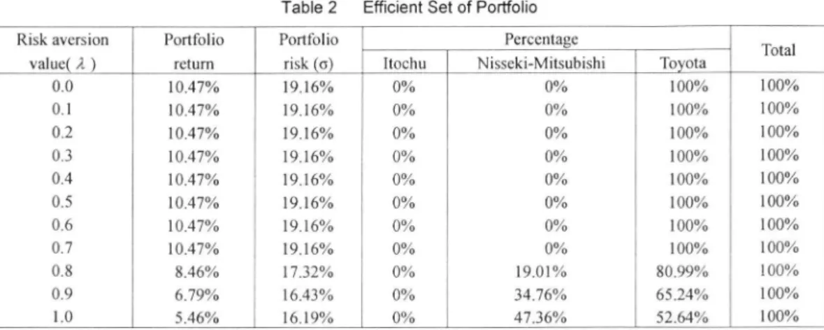
Nisseki−Mi 0% 17.0% 19.0% ←2LO% 23Table 2 Efficient Set of Portfolio
Risk avcrsion Portfblio PortR)lio Percentage
Total
va1UC(λ) return risk(σ) Itochu Nisseki−Mitsubishi To ota
0.0 10.47% 19.16% 0% 0% 100% 100% 0.1 10.47% 19.16% 0% 0% 100% 100% 0.2 10.47% 19.16% 0% 0% 100% 100% 0.3 10.47% 19.16% 0% 0% 100% 100% 0.4 10.47% 19.16% 0% 0% 100% 100% 0.5 10.47% 19.16% 0% 0% 100% 100% 0.6 1047% 19.16% 0% 0% 100% 100% 0.7 10.47% 19.16% 0% 0% 100% 100% 0.8 8.46% 17.32% 0% 19.Ol% 8099% 100% 0.9 6.79% 16.43% 0% 3476% 65.24% 100% 1.0 5.46% 16.19% 0%
4736%
52.64% 100% Source:Author’s calculation. Table 2 shows the various efficient portf()lios with each pair of portfblio retum and risk including the ratio ofeach stock in the portfblio corresponding to the degree of aversion to risk(i。e. selective risk aversion values from O to l). In the global minimum variance portfblio(λ=1), the solution by quadratic programming places 4736%of the investor’s money in Nisseki− Mitsubishi and 52.64%in Toyota. On the other hand, in the maximum return portfolio(、孔=0), the solution places IOO%ofthe investor’smoney in Toyota. Figure 2 Risk Aversion and Portfolio Choice Composition of Efficient Portf{)lios 19876543210000000000
ぱ“♂“““・s講ぷぷぷ♂ぱ試評ぷ
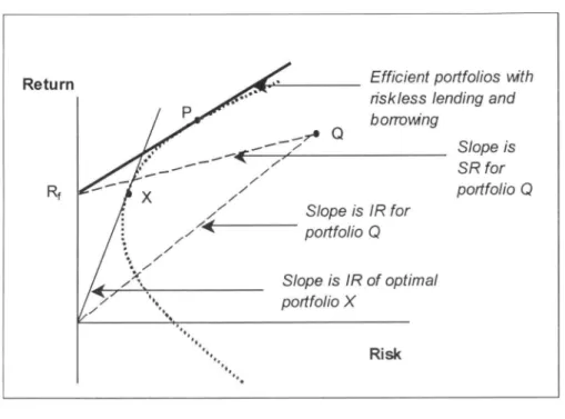
Ri・kA…si・・V・1・・の \ ー Source:Author’s compilation.Stochastic Mean−Variance Optimization in Portfolio Analysis According to Table 2, the moderate risk averse investor allocates all his money to Toyota and the very risk averse investor(λ>0.7)diversi丘es his money into Nisseki−Mitsubishi. The higher the risk aversion value, the larger the廿action of Nisseki−Mitsubishi in the efficient portfblios(Figure 2)・ Interestingly, Itochu is not included in the efficient portfblios, even though Nisseki−Mitsubishi with a negative expected retum is included in the efficient portfolios selected by the very risk averse investors. This stems廿om the fact that the stock retums of Itochu were relatively highly correlated to those ofNisseki−Mitsubishi and Toyota as shown in the correlation matrix in Table 1. The correlation coefficient between Toyota and Nisseki−Mitsubishi is approximately O.386, much less than those between Toyota and Itochu,0.636 and Itochu and Nisseki−Mitsubishi,0.739. It is note that the benefits of diversification are essentially due to the combination between assets with low(or, if possible, negative)correlation. In this point, the covariance matrix that concisely contains all necessary information about volatility and correlation statistics plays a key role in forming efficient portfolios. To construct an efficient portfolio, it is necessary to include inefficient assets because the risk of an individual asset should be of little importance, but its contribution to the portfblio’s risk as a whole should be taken into account fbr the investor. There are some risk−adjusted performance measures(RAPMs)which take account of both risk and retum characteristics fbr portfblio construction. The Sharp ratio and the infbrmation ratio are two of the standard RAPMs fbr investment analysis. The most common R.APM is the Sh・叩・ati・・whi・h i・c・mp・t・d・・the excess ret・m・v・・th・・i・k一廿ee・at・, R.f di・id・d by th・ volatility ofthe asset(or port五)lio). Mathematically,
SR−(∫∼・:1∼ル (24)
(l where Rq andσq are an arbitrarily chosen portfblio retum and risk This is given graphically as the slope of the dotted line from the point of 1∼∫on the vertical axis in Figure 3. The Sharp ratlo is applied in the case ofallowing un]imited riskless lending and borrowing as a risk−free rate. Ifrisk一廿ee retums are assumed to be zero(or, no risk一廿ee asset exists), the appropriate RAPM is the infbrmation ratio given by the slope ofthe dotted line from the origin to the point Q,Figure 3 Risk Adjusted Pe㎡omance Measures Efficient portfo/’os vw’th 刀sk∫ess∫θηd’ηg aηd borroWi’ng S∫oρe∫s/Rfor portfolio Q Stope is/R of opt’ma∫ portf()∫io X Sloρe is SR for portfoiio Q Source:Alexander[20011, p.193.
・R−≒ (・・)
These RAPMs indicate the measures of reward per unit of risk. How can these ratios help us in constructing an optimal portfolio? According to the mean−variance optimization rule, investors seek to maximize the portfolio retum fbr a given portfolio risk. In either case, fbr a given volatility(risk),σq,investors want the rate ofretum to be as great as possible, that is, they need to choose the solid line with the greatest possible slope. In the case ofthe above numerical example, the maximum infbmation ratio is O.5466, in which the portfolio is solely composed of the stock ofToyota(100%). Finally, in our simple numerical example, the stock ofToyota has a huge e ffe ct on the shape of the efficient fヤontier and the construction ofoptimal portfblios, particularly fbr an investor who is not very risk−averse. This is because Toyota has a much higher retum than that of the other two stocks. In the practical application of mean−variance optimization it is quite common that optimal portfolio will be dominated by just a few assets with high−retum, high−risk characteristics㌧ lAlexander[20011 indicates the predominant e廿セct of a fヒw high−risk, high−retum assets on the shape of the e缶cient 倉ontier among 35 assets. P.199.Stochastic Mean−Variance Optimization in Portfolio Analysis
4.Stochastic OptimiZation by Monte Carlo Simulation
In the previous section, I explained the mathematical setting of mean−variance optimization problem and provided a simple numerical example fbr depicting the efficient frontier in the context of a trade−off between risk and retum The solution to the quadratic programming problem is to find a set of values fbr the decision variables, w, that optimizes the associated o句ective. All data(expected retums, volatility and correlation statistics)used in the model were calculated from historical performances of the individual stock retums, that is, they are inpu廿ed as constant variables. This makes the model deterministic. However, decision making in portfblio analysis essentially involves ex ante retums(Le., future performances)and uncenain巧of these retums has to be quanti行ed in the optimization process. In this regard, ex ante(in the original meaning ofthe”expected”and uncertain)returns can only be described probabilistically. his worthwhile to note that the method of optimization should be selected out of those renecting the original theoretical insight in the Markowitz mean−variance analysis. Markowitz [1952]pointed out that”Our suggestion as to tentativeμ、, σびis to use the observed μ∫, σ〃 fbr some period of the past. Ibelieve that better methods, which take into account morein品㎜ation, can be fbund. I believe that what is needed is essentially a=
一(emphasis mine)in the last part ofhis seminal article.
Monte Carlo simulation is a povverful technique fbr analyzing models involving probabilistic assumptions. In a stochastic optimization model, the simulation assumptions capture the uncertainty of ex ante retums using probability distribution and fbrecasts of the o句ective will also have some probability distributions of possible results fbr the model. The central idea behindMonte Carlo simulation is based on repeated random sampling廿om a given probability
distribution that is assumed to model inputs to characterize the distributions of model outputs. Crystal Bal1, which I wnl employ as an optimizer in this section, is one of the popular programs of Monte Carlo simulation. The process of Monte Carlo simulation using Crystal Ball is roughly divided into three steps:品㎜ulating the spread−sheet model to solve the problem, identifying probability distributions of input variables to generate random numbers, and implementing Monte Carlo simulation to evaluate the outcome廿om the distribution ofmodel output. The spread−sheet model used in Crystal Ball is the same as the model of quadratic programming in Section 3. The historical data used in the simulation is the same three stocks as in Table l. Probability distributions of input variables to generate random numbers are normal distributions fbllowing the nomal distribution hypothesis behind the Markowitz mean−varianceanalysis. In a dete㎜inistic optimization, three maj or elements of the model were decision variables, constraints and an objective. Astochastic optimization model has additional elements: the simulation assumptions about probability distributions used to generate model data and the f()recasts expressed as the frequency distributions of possible results for the model. Table 3 Summary of Mean−Variance Optimization Deteministic Optimization Stochastic Optimization <Monte Carlo Simωation> <Quadratic Programming>
Nomal
Student−t 「lobal nlinilnun variance portfblio Retum(Mean) 5,463% 5,448% 5,450% Risk(SD) 16,186% 16,194% 16,194% Composition Itochu 0.00% 0.00% 0.00% Nisscki−Mitsubishi 47.36% 47.49% 47.47% Toyota 52.64% 52.51%5253%
Probabihty ofapositive retum * 62.00% 61.75% Min Max Min Max 90%Certainty Range * 一20.892% 31.247ツ 一23.271% 33.391% 95%Certainty Range * 一26.878% 34.694{※ 一30.273% 38.1029% 99%Certain呼Range * 一36.100% 40.870% 4L445% 46254% 100%Certainty Range * 一37376% 51.700「% 一44.657% 57.890% Downside 10%Range * 一14.533% 一15,830% Downside 5%Range * 一20.892% 一23.271% Downside 1%Range * 一29,786% 一33.659% Maximum infbmation ratlo portfblio Infbrmation ratio05466
05466
0.5466 Rcturn(Mean) 10467% 10,467% 10,467% Risk(SD) 19,148% 19,148% 19,148% Composition Itochu 0.00% 0.00% 0.00% Nisseki−Mitsubishi 0.00% 0.00% 0.00% Toyota 100.00% 100.00% 100.00% Probability ofapositive retum * 70.66% 70.21% Min Max Min Max 90%Certainty Range * 一21.394% 4L651% 一23.690% 43.825『〃 95%Ceれainty Range * 一27264% 47.675% 一30.857% 51」339% 99%Certainty Range * 一39990% 57.788「% 一48210% 64.599% 100%Certainty Range * 一45318% 82.160「% 一56.441% 106960「% Downside 10%Range * 一14,133% 一15355% Downside 5%Range * 一21.394% 一23.690% Downside 1%Range 一 * 一35260% 一4L415% Source:Author’s calculation.Stochastic Mean−Variance Optimization in Portfolio Analysis The results ofthe experiments are summarized in Table 3, and the outcomes ofthe simulation are provided as frequency charts of model output(Figure 4). In contrast, deterministic
optimization fbr the global minimum variance portfblio(GMVP)provides only one value of
portfblio renlm 5.463%and risk 16.186%, since all data are inputted as constant variables. The solution to the global minimum variance portfblio under stochastic optimization has a po rt f()lio risk of 16.194%(standard deviation)and a portfblio retum of 5.448%, in which O%of the investor’s money is allocated to Itochu,47.49%to Nisseki−Mitsubishi and 5251%to Toyota. By manipulating the end−point grabbers or by changing the range and certainty values in the boxes in the fヤequency chart(Panel B ofFigure 4), we can specify a certainty level or a probability interval of realizing the global minimum variance portfblio retum. For example, the probability of a positive return is 62・00%. In case ofthe result of changing the certainty level to l OO%, the rangecentered about the mean is廿om−37.376%to 51.7%compared to that of the maximum
infbrmation ratio portfblio廿om−45.318%to 82.160%(Table 3). It is clear that the global minimum variance portfblio has a smaller range of expected retum compared to the maximum information ratio portfolio(MIRP). Figure 4 Forecast of Monte Carlo Simulation PanelA GIobal MinimumVarlan㏄Port↓ob…おr Nomヨ Maximum h「ormation Ratio Por廿()歓)臨ト㎞md 0〔5 004≧’ i三〇c32
β・Ω OO1 。,ft>1・ 005 et・ o Pt 芸。、, 亘 £。〔: 001 0[D .reア27%.t3.S6SU O.αd眺 13.363se rs727%40⑭% Return GMVPunder Norma1:Prob. of Posit iVe Return = 62.㎜ D .訪.721% _1〕託3% C[ooeb 13斑3% ?67?7% Return 28 24 烈 16 12 8 4 田40 53454% 印2FδコQ Panel B 市﹁25コO 2e @24 抽 16 η 8 4 4。銭 45 ■3 5L
% 蜘 40 0口5 eo4言‘ 三、。3 8 2 全 002 001 0⑥ 0.05 004 .言 云a。38
2 ec OO2 001 0m 27 24 ?1 ]8甲 2 15ξ 1ユヨ Y 9 5 ] ・ ・40 .40 ㎜ ^n ㎜ 0 ㎜ 刀 眠 40 鵬 50 [mo% 80 眠 Retum MIRPunderNormal:Prob. ofPos面∨eRetum=70.〔胱 .40 ⑭% .ro oa]% Return ?7 24 ?1 18 1i 3 1s亘 12・2 9 6 3 ・ ・〈o &〕pm)% ξ〔come To sum up, stochastic optimization provides us with forecasts of our objectives probabilistically. In addition, we can get some insight about alternative measures of financialrisk, such as value at risk(VaR)and the expected tail loss(ETL)f㌔om our probabilistic fbrecasts of Monte Carlo simulation(fbr a more detailed explanation about VaR and ETL, see Dowd [2002D. In particular, it might be possible to provide a much better approach to allow the retum distribution with non−normality to be less restricted.
5.StyliZed Facts about Retum Distributions
The result of Monte Carlo simulation depends crucially on the probability distributions that will be assumed to generate the data ofrandom sampling. Ifsome unrealistic assumptions have been made in the data generating process, the simulation experiments will not give a precise answer to the problem. In the context of mean−variance optimization, the optimal asset allocation obtained廿om a simulation will not be accurate ifthe data generating process assumed normal distribution while the actual returns series is not normally distributed. The norrnal distribution hypothesis behind mean−variance analysis was based on the fact that asset retums are influenced by many different independent facts2. However, since the early l 960’s empirical research on returns distributions has almost universally fbund that such distributions are characterized by the features of the fat tails and high peakedness−excess kurtosis−and are ofモen skewed. Those features are known as stylized facts about financial return series, especially high 1予equency data. Table 4 represents descriptive statistics of historical perfbrmances of annual and monthly retum series(ltochu, Nisseki−Mitsubishi, Toyota and market)fbr a fifty year period from l 955 to 2004and a fifteen year period from l 987 to 2001. One of the features which stands out most prominently from the last columns is that the kurtosis of the fbur series is much higher than the normal value,3. This re刊ects the fact that the tails of the distributions of these series are fatter than the tails ofthe normal distribution. Put differently,1arge outlying(i.e. very small and very large)observations occur with rather high−frequency. Next, three individual stock return series have positive skewness. The skewness of the normal distribution▲s zero because its distribution is symmetric. Positive skewness implies that the right tail of the distribution is fatter than the le恒ai1. That is, large positive retums tend to occur more often than large negative ones. Positive skewness has an important impact on portfblio choice because it means that these stocks have a larger probability of very large payoffs, 2According to probability theory and statistics, any phenomenon made up of a large number of independent or weakly dependent variables has a normal distribution. See Focardi&Fabozz[2004], p,194.Stochastic Mean−Variancc Optimization in Portfolio Analysis Tab|e 4 Descriptive Statistics of Stock Return Series 〔%〕 1955−2004:Annual tochu isseki−Mitsubishi oyota arket l955−2004:Monthly tochu isseki−Mitsubishi oyota arket l987−2001:Monthly tochu isseki−Mitsubishi oyota arket
Mean
MedianMaximum Minimum
Std. Dev. Skewness Kurtosis17.628 15.994 23.254 14.776 1.433 1.368 L891
0909
0.381 0.043 0.778 0.022 10.700 7.300 19.200 15.950 0.000 0.000L200
0.800 一〇.800 −0.950 0.500 −0.400 240」00 144.800 110.600 72.100 72.700 52.000 46.80017500
60.000 36.800 43、100 17,500 一43500 −30.500 ・37.900 −24.800 一38,100 −28.900 −25.000 −19.800 ・38.100 −28900 −20.000 −19.800 46.093 34.982 33.087 19.956 11.Ol7 10.214 9.287 5.058 12.982 9.657 8.128 6.037 2.5271374
0.617 0,356L412
1.026 0.772 −0.130 1.049 0.299 1.002 0.09212364
5.478 2.942 3.271 9.220 6.330 5.040 3.934 6.968 4.617 7.028 3.534 Source:Calculated on the basis ofdata drawn f}om Japan Securities Research lnstitute, Kabushiki toshi shuckiritsu(Stock Retum Statistics). thus, they should have a preference f()r positive skewness. The monthly market retum series fbr the period of l955 to 2004 has only slightly negative skewness. It implies that large negative retums tend to occur more o丘en than large positive ones. It is clear that the distributions of all stock retum series Iisted in Table 4 diverge considerably from the nomlal distribution, have fatter tails, are more highly peaked, and are often skewed. The use of a normal distribution assumed fbr the data generation process in the simulation is likely to lead to a systematic underestimate of the occurrences of both sides of extreme values of retums. This is because they are more likely in practice than would arise under a nonnal distribution. One approach to remedies fbr stylized facts, especially fbr the tail’s parts of retum dis仕ibutions, is the replacement of the dis廿ibution assumed in the simulation from a normal distribution by a Student t−distribution. AStudent t−distribution is a symmetric and bell−shaped distribution similar to a normal distribution, but with fatter tails and a smaller peak at the mean. We have summarized the results of Monte Carlo simulation under the di ffe re nt assumed dis廿ibutions in Table 3 and Figure 5. The information demonstrates that the use of a normal distribution under the simulations leads to a systematic underestimate of the tai1’s parts offorecasts about the global minimum variance portfolio(GMVP)and the maximum in品mation
ratio po品)1io(MIRP), as extremely large positive and negative retums are more likely in practice than would arise under a normal distribution.005. 004・≧ ≡・as窒 £… 0.01 Figure 5 GM∨P underNormal:Downside 1.5and 10%Range
叫>L
.26.727%.1コis3se O.〔mo% 13.ad3SS 26ア27%4〔.oee% Retum GMVP under Student t:Downside 1、5and 1096 Range OO6 .. 0.05 .. .吉oo4.三 80田9 △r OO2 00∼o吟凸
奄ts6ec 、④77践 .15385% 0㎜ t5.3esSC 刃ア7crSt 略t託% Retum Forecast of Tail’s Part Pane|A MIRPunderN◆rmat:Downside 1,5and lO%Range 泌 24 市﹁2Fおコ皇 エ ー6 12@6
4 0 4糾 4 薗53 2B 24 20 16 12 8 4 田40 Panel B 市﹁B5コΩ 0[5 . 004 .ξ
⊇oo38
占eee OOl o[φ .40㎜ ,加㎜ ecrn% 20〔ume 40.[疏 60晒 Return MIRPunder Student t:Dowmside 1.5 and 10%Range 007 006 005≧』 三e.・4. ぽ 含oo3已 002 .. . 001 0〔φ・・ 与o〔㎜ ・釦㎜ 0晒 30㎜ 60000% Retum ■ ?T 24 ?t IBT 窒 15 己 2 12Q 9 6 3 ・ ・40 80㎜ 9.㎜ 3? 刀 ?4 幻 15 12 8 4 ■〈8 ﹁﹁B⊂o An altemative approach to overcome styhzed facts about retums distribution would be to use bootstrapping. ln Monte Carlo simulation, the data are generated completely artificially from the assumed distribution. On the other hand, bootstrapping does not assume some preset distribution but uses the actual data themselves. However, Brooks[2002】points out that there are at least two sltuatlons where the bootstrap will not work welL First, if there are outliers in the data, the conclusions of the bootstrap may be affected. Second, use of the bootstrap implicitly assumes that the data are independent ofone another. Ifthere were autocorrelation in the data, this would obviously not hold.6.Concluding Remarks and Future Direction of Research
In this article, we have considered the implementation of the mean−variance optimization in portf()lio analysis. The mean−variance analysis suggested by Markowitz is theoretically based on the expected utility theory and the normal distribution hypothesis about return distributions. The worth of the analysis rests on revealing normative rules for optimal portfolio choice by an individuaL The theory is relatively straightf()rward, however its implementation can get qulte complicated. Recently, remarkable progress has occurred in the area of risk management. Breakthroughs in its implementation制1 into two categories:an optimizer and a retum f()recast. In order to get robust results, these issues are crucial and closely related to each other.Stochastic Mean−Variance Optimization in Portfolio Analysis Ibegan with formulating the problem of mean.・variance optimization in a formal mathematical context and then demonstrated that a covariance matrix is a comerstone of risk reduction through portfolio diversification. Next, we implemented mean−variance optimization by using the methods of Monte Carlo simulation, which is consistent with the original idea of Markowitz’s approach in an aspect of probabilistic setting about retum fbrecast. The result of simulation relies mainly upon the assumed probability distribution to generate retum data in the model. Its robustness depends on whether the actual return distribution is fitting to the assumed distribution under simulation. According to the historical performance ofretUrn series, the retum distributions are not normally distributed. To rectify the results of simulation to tail’s parts of return distributions, I added to implement the simulation under the assumption of Student t− distribution and pointed out the posslbility of using the method ofbootstrapping. These methods are directed to improve the assumed distribution under simulation in an aspect of curve fitting to actual retum distributions. In other words, I attempt to fit an assumed distribution to historical data unconditionally. More fUndamentally, practical problems with mean−variance optimization lie on the use of return data. Three key ingredients in portfolio optimization are a return forecast, an optimizer and a utility function. A,lthough those are inseparable from each other, an accurate retum f()recast is of paramount importance on data input in the optimization process. The covariance matrix provides concise and precise information about volatilities and correlations as discussed in Section 2. Volatility and correlation are parameters of the stochastic process that are used to model the variation in asset prices. The estimation and fbrecasting is at the heart of mean− variance optimization. In practice, they are not directly observable, unlike asset prices. They can only be estimated in the context of a statistical model, and those estimates depend on the choice of model applied to historical retum series. Campbel1, Lo and MacKinlay[1997]state that nonlinear characteristics in economic behavior might be fbund in financial markets, fbr instance, investor’s attitudes toward risk and expected return, strategic interactions among market participants. The inforrnation stemming from nonlinear characteristics is incorporated into asset prices, the dynamics of which are embodied in the stylized facts after all. The stylized facts implying leptokurtosis and volatility clustering lead us to consider the introduction of nonlinear models such as GARCH models and so on to describe the observed patterns in stock retum series.
References
Alexander, C.[2001],Market Models: A guide to Financial Data Analysis, John Wiley, Chichestcr. Amenc, N、 and Sourd, V. L.【2003], Porグb∼’07乃θoワαη4 Pθヴbrmance Analysis, John Wiley, Chichester. Brooks, C.12002】, lntroductoり・ Econome’r’cs/br Finance, Cambridge University Press, Cambridge・ Camm, J. D. and Evans, J, R.[2000],Manage〃len’Science and Decision Tecんη010gソ, South−Wcstern College Publishing. Campbell, J. Y., Lo, A. W. and MacKinlay, A. C,[19971, The Econometrics()f Financia’Mo舵’s, Princeton University Press, New Jersey. Dowd, K.[20021, Measuring Market Risk, john Wiley, Chichester. Elton, E. J. and Gruber, M. J. I l 9951, Modern Porグblio 7乃θoワαη4伽eぷtment Ana!ys’∫,5th ed., John Wiley, Chichester. Fabozzi, F, J., Gupta, F. and Markowitz, H. M.[2002],“The Legacy of Modem Portfblio Theory,” @ノournal(ゾ Inveぷting, Fal1, pp.7−22. Facardi, S. M. and Fabozzi, F. J.[2004], The Mathe〃laticぷ()f Fiuancial Mbdeling and lnvetment〃urnage〃len’, John Wiley, Chichester. Franses, P. H. and Dijk, D. V.12000],∧Jonイinear Time Ser’es Modets in E〃rpirica/F’nance, Cambridge University Press, Cambridge, Glantz, M、[2000],Scienti:f}c Financialルlanagemen’, AMACOM, New York. Greene, W. H.12000】,Econometric Ana!ys’ぷ,4th ed., Prentice−Hall, Inc, New Jersey. Jocobsen, B, and Dannenburg, D.12003].“Volatility Clustering in Monthly Stock Retums,” @ノournal of E叩’r’ca/ Finance, Vol.10, pp.479−503. Jobst, N. J., Homiman, MD., Lucas, C.A. and Mitra, G,[2001],‘℃omputational Aspects of AhemaUve Portf()lio Selection Models in the Presence of Discrete Asset Choice Constraints,” ρuan’itative Finance, Vo1」, No.5, pp.489−501. Kallberg, J.G. and Ziemba, W. T.[1983],“Comparision of Altemative Utility Functions in Po疏)lio Selection Problem,” ルlanagement Sc)ence, Vo1.29, pp.1257−1276. Laws, J,[2003], ‘‘Portfblio Analysis Using Exce1,◆’ ln!4〃hedρuantitativeルfe’hods/br Trading and/nvestment, C. Dunis, j, Laws and P. Naim(eds), John Wiley, Chichester, pp.293−311. Ledoit, O. and WoばM.[2003],“lmproved Estimation ofthe Covariance Matrix ofStock Retums with an Application to Portfblio Sclection,” Journal()fE〃rpir’ca∼F元na〃ce, Vo1.10, Issue 5, PP.603−62 L Lhabitant, F−S.120021, Hedge Funds, John Wiley, ChichesteL Markowitz, H.[1952],‘’Portfolio Selection.” Journal〔)fFina〃ce, VoL7, pp.77・91. Munechik凡M。[2002],“Foundations of thc Mean−Variancc Analysis:Normal Distribution Hypothesis and Expected Utility,” Economic 1∼eview〈ゾアbッo Universめノ, VoL28, No.1,pp.51−87.Stochastic Mean−Variance Optimization in Portfblio Analysis Mills, T, C.[1999】,η昭Econo〃retric〃b凌〃ing()f Fina〃cial Ti〃le Ser’es,2nd. ed., Cambridge University Press, Cambridge. Mun, J.12004],4〃〃ed Risk Analyぷ’ぷ, John Wiley, Chichester. Ragsdale, C. T.[2001】, Spreadsheet〃bdeling and 1)eciぷion Analyぷis,3rd. ed., South−Westem College Publishing, New York. Ross, S. A., Wester行eld, R. W. and Jaffe,工[19961, Corporate Finance,4山ed., McGraw−Hill Companies, Inc. Chicago. Ruppert, D.[2004],Statiぷtics and Fi〃ance:.4η」rntroduction, Springer−Verlag, New York, Sharpe, W F.[1963】,“A Simplified Model for Portf()1io Analysis,”〃bnage〃len’Scie〃ce, VoL9, pp.277−293. Stevens, G V.【1998],“On the Inverse Covariance Matrlx in Porf()1io Analysis,” Journal of Finance, VoLLm, No.5, October, pp.1821−1827. Teall, J. L. and Hasan,1.[2002j,ρuantita’ive Methods/br F’nance and/hves〃nents, Blackwell, Oxfbrd. Teall, H.[1983],“Linear Algebra and Matrix Methods in Econometrics,” in Handbook()f Econome tr’cs, Vol.1,Z. Griliches and M. Dコntriligator(eds.), North−Holland, Amsterdam, pp5−65.