「文藝と思想」第 78 号 2014 年 2 月 (79) ~ (102) 頁
Rasch Analysis and Rating Scale Analysis
J. LAKE
AbstractThis study presents an introduction of Rasch analysis through theoretical and mathematical explanations. Guidelines and suggested values are presented for different aspects of an analysis. Rating scale analysis as a special type of Rasch analysis is introduced and additional suggestions for scale development are made. Both individual item analysis and whole scale analysis are discussed. In study 1, a practical example of rating scale analysis is demonstrated by showing the develop-ment of a measure of second language (L2) writing interest. Some items are shown to be of poorer quality and the scale is revised. In study 2, the revised scale is shown to have good measurement properties as observed in the item and scale analysis. Additional validity evidence is provided beyond scale properties by showing that the measure of L2 writing interest has a positive relationship with L2 writing motivation and a negative relationship to L2 writing anxiety.
Rasch Model Introduction
In classical test theory item and examinee statistics are sample dependent. In other words, statistics about groups of examinees will change with differing groups. For example, for one group you might get a reliability coefficient of .95 and for another group .65. Even though researchers talk in a short-handed fashion
about test reliability, there is really no such thing as a reliable test, that is, in clas-sical test theory reliability refers to the data produced by a particular group (Thompson, 2003). Item statistics also have the same characteristics of changing with differing samples. Also, in classical test theory, statistics about people change with differing items. This dependence on samples of items and people pose a problem for measurement. Imagine if using three different measures of length or the same measure over three occasions for a person’s height gave readings of: 170 centimeters, then 150 centimeters, and then 180 centimeters. Measurement would be inconsistent and thus impossible. This was the problem George Rasch solved. Rasch developed a model based on a concept of specific objectivity that provides measurement invariance (Engelhard, 2013; Rasch 1960/1993; Wright, 1977). Measurement models and analysis using his insights are called Rasch models.
Rasch models provide item and examinee statistics that do not depend on any particular set of items or examinees, that is, they are sample independent. Invariance solves many measurement problems. With invariant measurement it becomes possible to monitor test or item quality and person or group measure-ment precision. Just as with measuring length, it is useful to evaluate the level of precision for different measurement purposes. For example, it may be satisfactory to measure the distance between cities in meters. For clothing, meters would be too imprecise and centimeters would be a better level of precision. Understanding Rasch models helps in test or scale construction (Wright & Masters, 1982; Wright & Stone, 1979). Solutions to other practical issues are relatively easy using Rasch analysis: item banking, test linking, measuring learning and development, placing students into similar ability groups, and making educational program decisions (Engelhard, 2013; Holster & Lake, 2012; Lake & Holster, 2012; Rasch 1960/1993; Wright, 1977).
Raw data from Likert type scales return ordinal data; however, one of the assumptions of parametric statistics is that the data be interval in form. Interval measures can be constructed by transforming the ordinal data from the scales by applying the Rasch measurement model. This model is a stochastic or probabilis-tic model that is based on the probabilities that a person will answer correctly or
endorse different items, or given an item, the probabilities that persons with differ-ent abilities will answer correctly or endorse that item. While the mathematics might seem complicated at first, further study reveals what Thorndike (1904) pointed out long ago about statistics, “There is, happily, nothing in the general principles of modern statistical theory but refined common sense, and little in the technique resulting from them that general intelligence can not readily master” (p. 1). The Rasch model is based on the conceptually simple idea that respondents with higher ability will have increasingly higher probabilities of answering cor-rectly, while items with greater difficulty decreases the probability of a correct response (Rasch, 1960/1993).
The Rasch model can be represented mathematically in different forms. The natural logarithm of the odds ratio in the Rasch model is modeled as the difference of a person’s ability level from the item difficulty. In mathematical form the log odds dichotomous Rasch model can be given by:
Logits = Log odds = ln[Pni/(1 – Pni)] = βn – δi Where :
ln = loge = natural logarithm or logarithm to the base e Pni = probability of success for person n on item i 1 – Pni = probability of failure for person n on item i βn = person n’s ability level and scale location δi = item i’s difficulty level or scale value
Natural logarithm of the odds or log odds are usually given in units called logits. The abilities of the respondents (also called persons) and difficulties of the items can then be mapped onto a scale with the same linear interval units. As can be seen by the formula, in the Rasch model items and abilities have specific objectiv-ity, that is, they are invariant over specific items or specific persons. Item difficul-ties can be generalized beyond the sample and person abilidifficul-ties generalized beyond a particular set of items. For example, in the case of person ability β1 and person ability β2 for an item difficulty of level of δi, the difference is:
ln[Pi1/(1 – Pi1)] – ln[Pi2/(1 – Pi2)] = (β1 – δi ) – (β2 – δi ) = β1 – β2
The item difficulty drops out of the calculation so the difference in the ability of person 1 and person 2 is invariant and does not rely on a particular item or set of
items. In the same way, it can be shown that the item difficulty does not rely on any particular person or set of person abilities.
Another form of the Rasch model is: Pni = e(βn – δi)/(1 + e(βn – δi))
Where:
Pni = probability of success for person n on item i βn = person n’s ability level and scale location δi = item i’s difficulty level or scale value
e = an irrational transcendental constant with a value of approximately 2.7183 This is known as the simple logistic Rasch model. This formula is also known as the one-parameter logistic model by researchers from an item response theory perspective that may include additional parameters; the one parameter in this case being item difficulty. From the Rasch perspective though, person ability is also modeled, so that at least two parameters are included in a Rasch analysis. Even though the formula is the same for one form of the Rasch model and the one parameter model, one of the main differences between the terminology is that an a priori decision is made in Rasch analysis to examine if the data fits the model, where with the one parameter model, the model is fit to the data and if it does not, other models such as the two- or three-parameter model may be used with further modeling to fit the data. Unlike the log odds form of the Rasch model, the relation-ship of probability to item difficulty or person ability is nonlinear. The stretched s-shaped curves of these relationships are called item characteristic curves or item response function curves. They are monotonic ogive curves, that is, they function in one direction with increased probability as points move up the curve.
In addition to a dichotomous model, the Rasch family of models also includes polytomous models for when there are multiple response options such as on a Likert-style rating scale. In this case, items consist of ordered categories with steps or thresholds between categories, for example, an item with six categories would have five thresholds between them. In mathematical form the log odds polytomous rating scale Rasch model can be given by:
Logits = Log odds = ln[Pnik/(1 – Pnik)] = βn – (δi + τk) Where :
ln = loge = natural logarithm or logarithm to the base e
Pnik = probability of success for person n on item i at threshold k 1 – Pnik = probability of failure for person n on item i
βn = person n’s ability level and scale location δi = item i’s difficulty level or scale value
τk = threshold difficulty at the kth intersection of category boundaries
In the rating scale model the threshold difficulties at the boundaries of the cat-egories are the same for all items on the scale in contrast to the partial credit model where steps between categories are allowed to vary. The number of param-eters to estimate in the rating scale model is thus much less than the number for the partial credit model. The person response estimate can be calculated by a combination of the item location and the threshold difficulty.
The probability form of the rating scale polytomous Rasch model can be given by:
Pnik = e(βn – (δi + τk)/(1 + e(βn – (δi + τk)) Where:
Pnik = probability of success for person n on item i at threshold k βn = person n’s ability level and scale location
δi = item i’s difficulty level or scale value
e = an irrational transcendental constant with a value of approximately 2.7183 τk = threshold difficulty at the kth intersection of category boundaries
The mathematical forms of the Rasch model show that it is possible to calculate estimates of person abilities that do not depend on a particular set of items and thresholds, and that it is possible to calculate estimates of scale values and thresh-olds that do not depend on a particular set of person abilities. This specific objec-tivity and the addiobjec-tivity for fundamental measurement gives Rasch analysts insights, such as: individuals’ responses to items, how the person is situated rela-tive to the group, items’ contributions to the measure, how information is orga-nized throughout the measure, and how the group is distributed relative to the measure.
Rasch Fit Statistics
When measuring something well, there is a paradox that the more precise you are measuring something, the more you should expect your measurement to contain some amount of error. In addition if you are aiming at measurement “truth”, you may get less error but the measurement will be less useful. For example, say I am measuring the heights of a group of people. I could be quite accurate with no error if I were to gauge heights within a meter of being accurate. If I were to gauge the heights with more precision, say, an estimate on a centimeter scale, my measurements might contain more error, especially with heights that are around the mid-centimeter mark. If I were to be even more precise, to say, the millimeter level, my measurements might often be in error even though they are quite precise. At the precision of the meter level, measurement might be “true” or “correct”, but the measurement would not be very useful. At the level of mil-limeter, measurement might be in error but it could be useful. Buying clothes at the meter level would be a poor fit to your body, buying tailored clothes even if in error at the millimeter level would fit your body well.
Real data differ from the theoretical, mathematical Rasch model as with any type of measurement. However, because both the data and model are known it is pos-sible to calculate differences between theoretical values and actual data. These differences can then be summarized over items or respondents indicating how well the data fit the model. The Rasch model is a probabilistic model so that data can deviate from the model by either deviating in one direction by not being probabi-listic “enough” or in another direction as being too random. In other words, data can deviate from the ideal probability (that models a certain amount of probabilistic variation) as being too ordered or absolute (lacking unpredictability or lacking sto-chasticity) or it can deviate by having too much unknown variance or “noise” (randomness). Data that overfit the model contain fewer probabilistic responses than predicted, and sometimes this is referred to as being deterministic or Guttman-like. Data that underfit the model contain more random responses than predicted. Model-data fit values are derived from residual difference from expected values and actual values in respect to the measurement scale.
If the expected value is subtracted from the actual value the result is the score residual.
yni = xni – Eni
A standardized residual can be calculated by dividing by the square root of the response variance or standard deviation of the actual score responses.
zni = xni – Eni/[pni(1 – pni)]1/2 = yni/SDxni
A fit statistic can be calculated by averaging the standardized residual variance for either items or persons.
Ui = sum of zni2 / N for n = 1 to N or, Ui = sum of (residual2/information)/N
This is the unweighed mean square fit statistic that is commonly called outfit mean square. This statistic is sensitive to unexpected responses that are rela-tively distant from the person’s or item’s measure, that is, a few unexpected responses far from the person or item scale location can cause misfit. Outfit is short for outlier sensitive fit.
A way to diminish the effect of distant unexpected residuals is to weigh nearby residuals so that they have more influence on fit. The squared residual can be weighed by its variance Wni.
vi = sum of zni2 multiplied by Wni divided by the sum of Wni for n = 1 to N. The variance can also be considered information so:
vi = sum of ((residual2/information)*information)/sum of information or, vi = average ((standardized residuals)2*information)
This is called a weighted mean square or infit mean square. Infit is short for information weighted fit. When item and person values are close the individual variance Wni is larger and when they are far apart the variance decreases lessening the impact on the infit mean square.
Infit and outfit mean squares are chi-square fit statistics divided by degrees of freedom that follow chi-square distributions, that is, they are not symmetrical around a mean but are positive values from 0 to infinity with an expected value of 1.0. However, infit mean squares and outfit mean squares can be transformed so that they can also be reported as standardized t values. For smaller N-sizes mean square fit statistics can be misleading by showing misfit due to the smaller sample.
Standardized t fit statistics can be a better gauge of fit. The values are analogous to z scores in that they have an expected mean of 0 and values plus or minus 2 are considered to be misfitting as they correspond to p values > .05. However, just as mean squares can be misleading for small samples, t fit statistics can be misleading for large samples. An N-size of 300 is suggested as a maximum value to evaluate misfit when using t values (Linacre, 2011, p. 515). As with most statistics, there are no absolute values that serve as a cutoff point. Instead when determining fit there are a number of points to consider so that items that might appear to misfit should not be carelessly discarded or items are retained merely because they appear to fit. Linacre (p. 514) suggest that mean square values between 0.5 and 1.5 indicate good item fit for rating scales.
PCA of Item Residuals
In addition to providing information about how data fit the Rasch model, item residuals can provide information relating to measure dimensionality. When mea-suring a single construct, it is expected that item variances relate to the one measure and that additional variance, if detected, is error. By definition random variance is error, or to put it another way, additional item variance is uncorrelated after extracting the variance due to the measure. An assumption in Rasch analy-sis, as in most statistical models is that measures are unidimensional (Gustafsson & Aberg-Bengtsson, 2012). Patterns in the residuals suggest that additional dimensions might exist in the data. One way to detect patterns is to do a principal components analysis (PCA) of the residuals.
Another assumption in Rasch analysis is that items are independent (Henning, 1989; 1992). In order for item measures to be additive towards a total score, each item must be statistically independent to function probabilistically. Dependence among sets of items suggests that additional dimensions are being measured (Wainer & Thissen, 1996; Yen, 1984, 1993). Dependence can also result from an item having an influence on another item (Jiao, Wang, & Kamata, 2007). If this is the case then these items will behave more deterministically than expected (Henning, 1989; 1992). Dependency of items also suggests a degree of
redundancy in sampling thus lowering construct representation and artificially increasing reliability. Excessive overfit can indicate dependence and correlations among item residuals can also indicate dependence.
If items are measuring on a different dimension beyond that explained by the measure this may be seen as unaccounted variance of the measure. A PCA of the item residuals is done to see if there is any patterning in the residuals that sug-gests an additional dimension. If item residuals have a strong component loading, that is, some item residuals are highly correlated, then this suggest the scale might not be unidimensional and further examination of the items might be neces-sary. Principal component eigenvalues can be rounded to a whole number that represents the number of items. Linacre (2011) suggested guidelines for detect-ing the existence of additional dimensions in the data:
• Variance explained by the measure should be at least 50%
• Eigenvalue units of unexplained variance in the first contrast should be less than 3.0 • Percentage of unexplained variance in the first contrast should be less than 10.0%. Reliability and Precision
In classical test theory (CTT), an important characteristic of measurement is reliability, that is, how consistently can a group be measured. In CTT observed score variance is equal to true score variance plus error variance and the reliability is the proportion of true score variance to error variance. Adding good items increases reliability because true score variance increase at a faster rate than error variance. When a range of items from very easy to very hard is given to large samples that have abilities from very low to very high, the patterns become more fixed. For example, the low ability people get the very easy items correct and the very high ability people get the easy up to the hard items correct. The patterns become fixed because the low ability people are getting the hard items wrong and the high ability people are getting the easy items correct. Obviously, however, when different people are taking a test this changes the variance observed so that reliability in CTT refers to the test scores of a particular group and not the test itself (Thompson, 2003).
For an individual member of a group, it is possible to calculate the standard error of measurement (SEM). Just as there is measurement error associated with the group scores, the SEM is the associated measurement around a particular indi-vidual score. The score is calculated by SEM = SD√1 – r , where SD is the stan-dard deviation of the scores and r = reliability. As can be seen from the formula, there is only one SEM for all the items in the test because it is based only on the standard deviation and the reliability. Therefore, SEMs are not consistent because they vary with different groups because standard deviations and reliabilities may vary.
From a Rasch analysis perspective or an item response theory perspective, what is important is the precision of the test at important points of difficulty for the construct being measured and precision in determining person ability. As Thissen and Orlando (2001, p.117) state, “reliability is frequently not a useful characteristic of an IRT scale-scored test.” Consistency or reliability for the group is not aimed at directly but is something like a by-product of precision. To gain precision, there needs to be a gain in information at the level difficulty or ability under scrutiny. (Information is sometimes referred to as information function, information curve or Fisher’s information (Embretson & Reise, 2000; Thissen & Orlando, 2001)). In CTT reliability describes group consistency, SEM describes consistency for an individual regardless of where the information in a test is located, Daniel (1999, p. 50) points out the contrast, “... IRT makes clear, in a way that reliability does not, that a test usually is more accurate for some members of a group than for others.”
In the Rasch model, the maximum information of an item is at the level of diffi-culty of the item. Item information is based on the person and item probabilities that are based on the person ability (β) and item difficulty (δ). The item informa-tion funcinforma-tion (IIF) can be described mathematically in different ways. IIF is equal to the derivative of the probability at a particular difficulty level squared, divided by the probability of getting the item correct multiplied by the probability of getting it incorrect, or more simply, it can also be calculated by multiplying the probability of getting an item correct (P) by the probability of getting it incorrect (Q) (Doran, 2005; Wright & Stone, 1979):
Q = 1 – P Which then gives us: Ii = P x (1 – P)
The test information function (TIF) at a particular difficulty level is the sum of the item information over all items for a specific difficulty level.
Standard Error of the Estimate (SEE) are analogous to the SEM in CTT. They are the inverse of the square root of the test information function, or:
SEE = 1 / (TIF)1/2
In fact, with Rasch analysis when the difficulty level and the ability level are equal, the probability of getting the item correct versus getting it incorrect are equal at .5 and the item information is at a maximum of .25 ((.5 x (1 – .5)) = .5 x .5). This ease of calculation might be one reason for the claim (Ostini & Nering, 2006, p. 30) that “test information is rarely employed in the Rasch measurement litera-ture where the issue of measurement precision is subordinated to issues sur-rounding measurement validity.” However, Luo and Andrich (2005, p. 324) state that, “Information functions are central in understanding the range in which a scale may be useful.” Even when raw scores are ultimately used, constructing test items using item information functions creates measures that give better precision and reliability than randomly choosing from an item pool (Davey & Pitoniak, 2006; Wendler & Walker, 2006). Because item information is near the same person loca-tion on the logit scale, a visual inspecloca-tion of the Wright map (Wilson, 2005) indi-cates if you have an adequate match between items and persons.
Rating Scale Effectiveness
In addition to investigating individual item statistics, it is possible to investigate scale statistics. As with item statistics, scale guidelines may vary so consideration of the purposes and stakes of the scale should be made. Guidelines considered here are based on Linacre (1999, 2002). Rating scales will be more effective if:
• There are at least 10 observations per category.
More than 10 may be necessary but this could be considered a minimum number. This is necessary so that estimates can be precisely calculated and for
scale measurement stability.
• Regular observations distributions.
Observations should not fluctuate widely between categories. This would suggest that respondents are interpreting some categories differently. Category distributions should be understandable in terms of what is being measured. If sharp variations are discovered, steps such as collapsing categories may need to be taken.
• Average measures should advance monotonically with categories.
This means that average person measures should be higher as categories increase in number. This simply means that in order to be functioning as a rating scale higher values should increase with higher categories or the scale is not working.
• Outfit mean squares less than 2.0
This refers to the category fit, not item fit. The interpretation is similar though with outfit values too high, there is too much noise in that category.
• Step calibrations advance.
Steps are the points where categories meet. They are sometimes referred to as thresholds, step calibrations, or Tau’s. As with average measures in categories, steps need to advance with increasing higher values for an interpretation that the scale is measuring something of increasing value.
• Steps difficulties advance by 1.4 logits with few scale categories, 1 logit with more scale categories
Three category items should have steps separated by about 1.4 logits for optimum scaling. For items with more categories a rule-of-thumb is that 1 logit indicate optimum separation. These separations are not a strict requirement. When met the steps can be considered to be similar to dichotomous items. This means that with optimal separation between steps more information is provided by each item.
• Step difficulties advance by less than 5.0 logits
If steps are too far apart it disperses the information provided by the steps. Precision is lost between steps. If steps are too far apart then individual items cannot optimally contribute to scale information. Respondents in the middle of the steps will have no matching items so they will have more measurement error. This effect is similar to reducing the number of items.
Illustrative Example of Rating Scale Development
Study 1. Interest as a characteristic of the second language writer introduction Developing second language (L2) writing ability may be important for students in academic contexts, for future career needs, or as a personal interest. Writing proficiency, especially the ability to write extended passages takes considerable time and effort to develop. Writing motivation is a key component in sustaining effort and persistence. As with other language domains, it is possible to distin-guish general to specific motivational concepts, such as broad stable motivational dispositions to the narrower contextual and dynamic motivational impulses (Lake, 2013; Lake & Holster, 2012). This study takes a positive psychology approach and looks at the domain of second language writing motivation to construct two scales. One is an Interest in L2 Writing scale that is related to L2 writing identity and another is an L2 Writing Self-efficacy scale that is related to L2 writing task moti-vation. Another scale, based on anxiety, a psychological component often found in models of the writing process (e.g., Hayes, 1996), is L2 Writing Anxiety. Relationships between L2 Writing Interest and L2 Writing Self-efficacy are hypothesized to be positive, and these two measures are hypothesized to have a negative relationship with L2 Writing Anxiety.
Writing interest has not been researched as much as reading interest in both first language and second language contexts. Most studies on writing interest are related to writing about interesting topics (e.g., Hidi & Anderson, 1992; Hidi & McLaren, 1991), while there are few studies on interest for writing (Lipstein & Renninger, 2007; Nolen, 2007). Interest in writing topics has been shown to have a relationship with writing quality (Albin, Benton & Khramtsova, 1996; Benton, Corkill, Sharp, Downey & Khramtsova, 1995). A study by Lipstein and Renninger (2007) showed how they were able to improve writing interest in their students. They point out that “it is important for educators to recognize that interest for writing can develop” (p. 140).
Self-efficacy beliefs in writing have been shown in numerous studies to have a strong relationship with writing performance (Pajares, 2003). Studies showing relationships between writing self-efficacy and writing outcomes have been done
with young students (Pajares & Valiante, 1997), high school students (e.g., Pajares & Johnson, 1996), and with college students (e.g., McCarthy, Meier & Rinderer, 1985; Meier, McCarthy & Schmeck, 1984; Woodrow, 2011). Writing self-efficacy beliefs have also been shown to have relationships with writing skills, strategies, and self-regulation (Pajares, Valiante & Cheong, 2007; Schunk & Swartz, 1993; Zimmerman & Risemberg, 1997).
L2 writing anxiety has been shown to have a negative relationship with L2 writing self-efficacy (Woodrow, 2011). Many L1 studies of writing self-efficacy have shown similar relationships (Klassen, 2002). In addition many L1 studies of writing anxiety have shown negative relationships with writing performance (e.g., Daly, 1978; Daly & Wilson, 1983).
The literature reviewed here supports the view that the three constructs of L2 writing interest, L2 writing self-efficacy, and L2 writing anxiety are important motivational constructs for writing. Scales measuring these constructs should show relationships similar to those described in the literature. It is important to develop precise measurements to describe the instructional environment and for possible use for future research in cross-group or within-group instructional treat-ments. It may be possible to identify types of writing instruction that improve motivation or decrease anxiety.
Participants
The participants in the first study are 133 first year female Japanese students in a public university in western Japan. Most of the participants were 18 or 19 years old. The selection of these participants was based on a convenience sample drawn from academic English writing classes taught by six different teachers. The par-ticipants were from three different departments: International Liberal Arts, Environmental Science, and Food and Health Sciences. The mean TOEFL score of the participants was 440 with a standard deviation of 20. The participants filling out the questionnaire were told that participation was voluntary, would not affect their grades, and promised that anonymity would be maintained.
Illustrative Measure Development
The motivational instrument used in this study was developed to measure second language writing interest. The L2 writing interest scale was created for this study derived from the theory and research writing interest using twelve items (e.g., “I am interested in writing in English”). The 6-item responses ranged from this is definitely not true of me to this is definitely true of me.
Results
Rasch analysis generates both total scale statistics and individual item statistics. Rasch analysis for this study was done with Winsteps software (Linacre, 2011). The Rasch person reliability coefficient was .87 and the Rasch separation index was 2.60.
In a dimensionality analysis the percentage of variance explained by measures was 62.1%. This was above the guideline of 50%. The eigenvalue units of unex-plained variance in the first contrast was 2.0, well within the guideline value of 3.0. The percentage of unexplained variance in the first contrast was 6.4%, well within the guideline value of 10%. For the scale as a whole then, this measure shows acceptable values for reliability and unidimensionality.
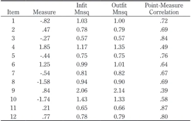
The Rasch analysis item statistics are presented in Table 1. As can be seen, only item nine is outside the guideline of 0.5 to 1.5 and severely misfits the Rasch model. Different guidelines have been proposed that take into account such factors as the type of test and the level of the stakes. If we use a more conservative value of misfit 1.3 then three items misfit: four, nine, and ten. It can also be seen that there is some redundant information in this scale represented by some overfit, for example, item three. Also, redundancy is indicated by items providing similar information with similar measure values, such as items nine and twelve. The point-measure correla-tion is similar to the point-biserial correlacorrela-tion in CTT except that this correlacorrela-tion is between the item and Rasch scale measures. These item statistics suggest that this scale could be improved by cutting items four, nine and ten, the three most misfitting items. These items also do not correlate as well with the whole scale.
Study 2. Measure internal, convergent, and discriminate validity evidence There were 284 participants in study two and they were of a similar background to the participants in study one. The new nine-item interest in L2 writing measure was reduced from twelve items by cutting the three misfitting items. The Wright map in figure 1 shows that the items were well targeted to the respondents. Item infit and outfit values were between the values of 0.6 to 1.4. The classical statistics for the scale were a mean of 33.94, standard deviation 7.61, and an alpha reliability of .90. The Rasch person reliability coefficient was .89 and the person separation index was 2.80. Although in this study there was only a small difference, Rasch person reliability is often a more conservative, more generalizable estimate of reliability than classical alpha reliability. This is because the ordinal nature and extreme scores for the raw data tend to inflate estimates compared to the interval nature of the Rasch measures. In the dimensionality analysis the percentage of variance explained by measures was 64.9%. This was above the guideline of 50%. The eigenvalue units of unexplained variance in the first contrast was 1.8, well within the guideline value of 3.0. The percentage of unexplained variance in the first contrast was 7.0%, well within the guideline value of 10%. For the scale as a whole then, this measure shows acceptable values for reliability and unidimensionality.
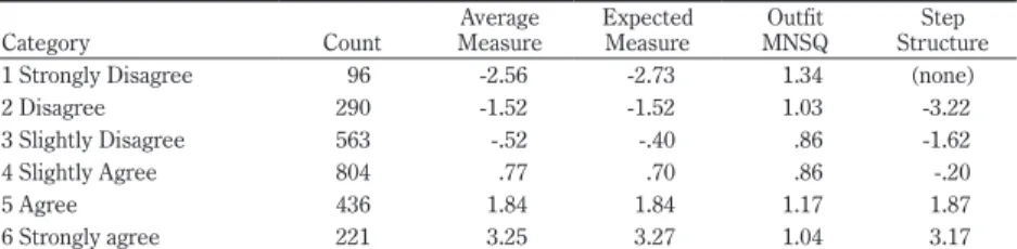
Rating scale structure statistics are presented in Table 3. As can be seen, the category with the fewest observations was 96 and this more than meets the guide-line minimum of 10. The observed values distribution has no abnormal
Item Measure MnsqInfit MnsqOutfit Point-Measure Correlation
1 -.82 1.03 1.00 .72 2 .47 0.78 0.79 .69 3 -.27 0.57 0.57 .84 4 1.85 1.17 1.35 .49 5 -.44 0.75 0.75 .76 6 1.25 0.99 1.01 .64 7 -.54 0.81 0.82 .67 8 -1.58 0.94 0.90 .69 9 .84 2.06 2.14 .39 10 -1.74 1.43 1.33 .58 11 .21 0.65 0.66 .87 12 .77 0.78 0.79 .80
<more>|<rare and difficult to endorse>
6 + # | | | | 5 + | | . | | 4 .# + | # T| ## | . | 3 + .## | .# | .## | .## | 2 .#### S+T ##### | .### | L2WI5 ####### | ##### | 1 .######### +S L2WI9 ######## | ######### | L2WI2 L2WI8 ####### M| ######## | 0 .####### +M ##### | L2WI3 ####### | L2WI4 ## | L2WI6 ###### | -1 .###### S+S L2WI1 .### | .# | #### | # | L2WI7 -2 # +T ## | # | .# T| . | -3 # + | . | | | -4 . +
<less>|<frequent and easy to endorse> EACH "#" IS 2: EACH "." IS 1
fluctuations and has more observations near the middle and fewer at the extremes. This suggests that observed values are appropriately distributed. Average measure values increase monotonically across all categories and observed measure aver-ages are near modeled expected averaver-ages. The category with the poorest outfit value is an extreme category with a mean-square value of 1.34, much less than the maximum guideline value of 2.0. Step calibrations all advance by more than 1.0 and less than 5.0. This meets the three guidelines about step advancement. All guideline recommendations have been met suggesting that rating scale structure is providing effective measurement.
In addition to measuring interest in L2 writing, two other measures were con-structed. One is a measure of L2 writing anxiety and another is a measure of self-efficacy of L2 writing. Second language writing anxiety was hypothesized to have a negative relationship with interest in L2 writing. Self-efficacy of L2 writing is a motivational variable that was hypothesized to have a positive relationship with the more dispositional identity-type of variable represented as interest in L2 writing.
The L2 writing anxiety scale had six items with the same response options as the interest scale. (Example item: I am anxious when I have to write a lot in
Category Count MeasureAverage ExpectedMeasure MNSQOutfit StructureStep
1 Strongly Disagree 96 -2.56 -2.73 1.34 (none)
2 Disagree 290 -1.52 -1.52 1.03 -3.22
3 Slightly Disagree 563 -.52 -.40 .86 -1.62
4 Slightly Agree 804 .77 .70 .86 -.20
5 Agree 436 1.84 1.84 1.17 1.87
6 Strongly agree 221 3.25 3.27 1.04 3.17
Table 3. Rating scale structure statistics
Measures k N Reliability Person
% of Variance Explained by Measures Eigenvales of Unexplained Variance in 1st Contrast % of Unexplained Variance in 1st Contrast
L2 Writing Interest (study 1) 12 133 .87 62.1 2.0 6.4
L2 Writing Interest (study 2) 9 284 .89 64.9 1.8 7.0
L2 Writing Anxiety 6 284 .75 59.8 1.7 11.4
L2 Writing Self-Efficacy 14 284 .89 53.8 2.1 6.9
English.) The L2 writing anxiety measure had a person reliability of .75 and a sepa-ration index of 1.75. The infit and outfit values were between 0.6 and 1.4. The dimensionality analysis showed that variance explained by the measures was 59.8%. The eigenvalue units of unexplained variance in the first contrast was 1.7. The unexplained variance in the first contrast was 11.4%. The reliability was low but could be accounted for in part by the few number of items. The unexplained variance in the first contrast was over the guideline figure of 10% but the eigen-value unit was in the acceptable range suggesting that this was not a problem and was sufficiently unidimensional. For the purpose of this study, the scale is ade-quately measuring L2 writing anxiety.
The L2 writing self-efficacy scale had fourteen items with the same response options as the interest scale. (Example item: I can write a well-organized para-graph in English.) The L2 writing self-efficacy measure had a person reliability of .89 and a separation index of 2.82. The infit and outfit values were between 0.6 and 1.4. The dimensionality analysis revealed that variance explained by the measures was 53.1%. The eigenvalue units of unexplained variance in the first contrast was 2.1 and the percent of unexplained variance was 6.9%. These values are within guidelines that suggest this scale is sufficiently unidimensional and for the purpose of this study it is measuring L2 writing self-efficacy well.
As can be seen in Table 2, the scale statistics improved between study one and two. Removing the three most misfitting items in the scale improved reliability and variance explained by the measures. This illustrates how piloted scales can be improved through the use of fit statistics.
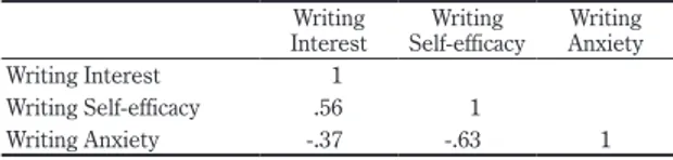
To provide some convergent and discriminant validity evidence the L2 Interest in Writing scale was correlated with the L2 Writing Self-efficacy scale and the L2 Writing Anxiety scale. Results are shown in Table 4.
Writing
Interest Self-efficacy Writing AnxietyWriting
Writing Interest 1
Writing Self-efficacy .56 1
Writing Anxiety -.37 -.63 1
As can be seen in the table L2 writing interest has a moderate correlation with L2 writing self-efficacy. This provides convergent validity evidence that there is a relationship between these variables but not so strong suggesting a degree of divergence so that participants can discriminate between them. Divergent evi-dence is also provided by the weaker negative relationship with L2 writing anxiety and the stronger negative relationship between L2 writing self-efficacy and L2 writing anxiety.
Conclusion
This study gave a theoretical overview of the Rasch model and how Rasch analysis is conducted. Guidelines were presented for doing Rasch analysis. One type of Rasch analysis called rating scale analysis was discussed in more detail. This study then used the development of an L2 interest in writing scale to illus-trate how the theory and guidelines can be used in practice to create a scale that provides invariant interval measurement. Guidelines were provided for both items and complete scale. To review, researchers developing a scale can check: Items by:
• Infit and outfit statistics. For low-stake scales, values between .5 and 1.5 are considered acceptable. For higher stakes or more precise measurements with less “noise” aim for values between .7 and 1.3. In general be more concerned with misfit than overfit.
• Wright map. Sometimes called the person-item map. For optimum precision the information for the scale needs to be distributed so that it roughly corresponds to the persons measured. This can be visually checked by checking to see that the items and persons are not too far apart or that the items are not bunched up so that you are getting redundant information.
• Point-measure correlation. This is the correlation of the item with the Rasch measure. If this is very low or negative then the item is not contributing measure-ment towards the scale as it should. If it is very high then this suggests that it may be overfitting, that is, providing redundant information. Given enough items, in general, be more concerned with very low correlations than high correlations.
Scales by:
• Rasch person reliability. This is similar to traditional measures of reliability but is usually more precise and generalizable.
• Rasch person separation. This gives a signal to noise ratio. If high, measure-ment impact diminishes the effects of noise. If low this suggests that there is too much noise to measure what is intended.
• There are at least 10 observations per category. More is better but for mea-surement stability 10 can be considered a minimum.
• Regular observations distributions. Respondents on average should be choosing categories in a patterned manner considering the purpose of the item and scale. Gaps or unexplainable fluctuations suggest further investigation.
• Average measures should advance monotonically with categories. The average person abilities should advance with increasing item category difficulty in order for the scale to be scaling properly.
• Outfit mean squares less than 2.0. As with item outfit values too high, outfit values that are too high in a category mean that there is too much noise in that category.
• Step calibrations advance. Steps need to advance with increasing higher values for an interpretation that the scale is measuring something of increasing value.
• Steps difficulties advance by 1.4 logits or more with few scale categories 1 logit or more with more scale categories. If steps are too close then perhaps fewer categories are needed.
• Step difficulties advance by less than 5.0 logits. If steps are too far apart then individual items cannot contribute to scale information and perhaps more catego-ries are needed.
Researchers often have a need to measure human traits and abilities as part of a study. Sometimes they need to compare groups of people, or show change in people through time. Interval level measurement that is invariant across people or time is critically important. This study technically explains and then practically demonstrates one type of analysis for creating such measurement in the hope that it will aid researchers in their research ability.
References
Albin, M. L., Benton, S. L., & Khramtsova, I. (1996). Individual differences in interest and narra-tive writing. Contemporary Educational Psychology, 21, 305–324.
Benton, S. L., Corkill, A. J., Sharp, J. M., Downey, R. G., & Khramtsova, I. (1995). Knowledge, interest and narrative writing. Journal of Educational Psychology, 87, 66–79.
Daly, J. A. (1978). Writing apprehension and writing competency. Journal of Educational Research,
72(1), 10–14.
Daly, J. A., & Wilson, D. A. (1983). Writing apprehension, self-esteem, and personality. Research
in the Teaching of English, 17, 327–341.
Daniel, M. H. (1999). Behind the scenes: Using new measurement methods on the DAS and KAIT. In S. E. Embretson & S. L. Hershberger (Eds.), The new rules of measurement: What
every psychologist and educator should know. (pp. 37-63). Mahwah, NJ: Lawrence Erlbaum.
Davey, T., & Pitoniak, M. J. (2006). Designing computerized adaptive tests. In S. M. Downing & T. M. Haladyna (Eds.), Handbook of test development. (pp. 543-573). Mahwah, NJ: Lawrence Erlbaum.
Doran, H. C. (2005). The information function for the one-parameter logistic model: Is it reliabil-ity? Educational and Psychological Measurement, 65(5), 665-675.
Embretson, S. E., & Reise, S. P. (2000). Item response theory for psychologists. Mahwah, NJ: Lawrence Erlbaum.
Engelhard, G. (2013). Invariant measurement. New York: Routledge.
Gustafsson, J., & Aberg-Bengtsson, L. (2010). Unidimensionality and interpretability of psycho-logical intruments. In S. E. Embretson (Ed.), Measuring Psychopsycho-logical Constructs: Advances
in Model-Based Approaches. (pp. 97-121). Washington, DC: APA.
Hayes, J. R. (1996). A new framework for understanding cognition and affect in writing. In C. M. Levy & S. Ransdell (Eds.), The science of writing: Theories, methods, individual differences,
and applications (pp. 1-27). Mahwah, NJ: Lawrence Erlbaum.
Henning, G. (1989). Meanings and implications of the principle of local independence. Language
Testing, 6, 95-108.
Henning, G. (1992). Dimensionality and construct validity of language tests. Language Testing, 9, 1-11.
Hidi, S., & Anderson, V. (1992). Situational interest and its impact on reading and expository writing. In K. A. Renninger, S. Hidi, & A. Krapp (Eds), The role of interest in learning and
development (pp. 215–238). Hillsdale, NJ: Lawrence Erlbaum.
Hidi, S., & McLaren, J. (1991). Motivational factors in writing: The role of topic interestingness.
European Journal of Psychology of Education, 6, 187–197.
Holster, T. A., & Lake, J. (2012). Developing an academic English program placement test: A pilot study. (Bungei to Shisou: The Bulletin of Fukuoka Women’s University International College of
Jiao, H., Wang, S., & Kamata, A. (2007). Modeling local item dependence with the hierarchical generalized linear model. In E. V. Smith & R. M. Smith (Eds.), Rasch Measurement: Advanced
and Specialized Applications. (pp. 390-404). Maple Grove, MN: JAM Press.
Klassen, R. (2002). Writing in early adolescence: A review of the role of self-efficacy beliefs.
Educational Psychology Review, 14(2), 173-203. doi:10.1023/A:101462680557
Lake, J. (2013). Positive L2 self: Linking positive psychology with L2 motivation. In M. Apple, D. Da Silva, & T. Fellner (Eds.). Language Learning Motivation in Japan. (pp. 225-244). Clevedon, UK: Multilingual Matters.
Lake, J., & Holster, T. A. (2012). Increasing reading fluency, motivation and comprehension through extensive reading. (Bungei to Shisou: The Bulletin of Fukuoka Women’s University
International College of Arts and Sciences), 76, 47-68.
Linacre, J. M. (1999). Investigating rating scale category utility. Journal of Outcome Measurement, 3(2), 193-122.
Linacre, J. M. (2002). Optimizing rating scale category effectiveness. Journal of Applied Measurement,
3, 85-106.
Linacre, J. C. (2011). Winsteps program manual. Chicago: Winsteps.com
Lipstein, R. L., & Renninger, K. A. (2007). “Putting things into words”: The development of 12-15-year-old students’ interest for writing. In S. Hidi, & P. Boscolo (Eds.), Writing and
motivation (pp. 113-139). Oxford: Elsevier.
Luo, G., & Andrich, D. (2005). Information functions for the general dichotomous unfolding model. In S. Alagumalai, D. Curtis, & N. Hungi (Eds.), Applied Rasch measurement: A book of
exemplars: Papers in honour of John P. Keeves. (pp. 309-328). Dordrecht, Netherlands:
Springer.
McCarthy, P., Meier, S., & Rinderer, R. (1985). Self-efficacy and writing. College Composition and
Communication, 36, 465-471.
Meier, S., McCarthy, P. R., & Schmeck, R. R. (1984). Validity of self-efficacy as a predictor of writing performance. Cognitive Therapy and Research, 8, 107-120.
Nolen, S. (2007). The role of literate communities in the development of children’s interest in writing. In S. Hidi & P. Boscolo (Eds.), Writing and motivation (pp. 241–255). Oxford: Elsevier. Ostini, R., & Nering, M. (2006). Polytomous item response theory models. Thousand Oaks, CA: Sage. Pajares, F., & Johnson, M. J. (1996). Self-efficacy beliefs in the writing of high school students: A
path analysis. Psychology in the Schools, 33, 163-175.
Pajares, F., & Valiante, G. (1997). Influence of writing self-efficacy beliefs on the writing perfor-mance of upper elementary students. Journal of Educational Research, 90, 353-360. Pajares, F., Valiante, G., & Cheong, Y. F. (2007). Writing self-efficacy and its relation to gender,
writing motivation and writing competence: A developmental perspective. In S. Hidi & P. Boscolo (Eds.), Writing and motivation (pp. 141–159). Oxford: Elsevier.
Rasch, G. (1960/1993). Probabilistic models for some intelligence and attainment tests. Chicago: MESA.
Schunk, D. H., & Swartz, C. W. (1993). Goals and progress feedback: Effects on self-efficacy and writing achievement. Contemporary Educational Psychology, 18, 337-354.
Thissen, D., & Orlando, M. (2001). Item response theory for items scored in two categories. In D. Thissen & H. Wainer (Eds.), Test scoring (pp. 73-140). Mahwah, NJ: Erlbaum.
Thompson, B. (Ed.). (2003). Score reliability: Contemporary thinking on reliability issues. Thousand Oaks, CA: Sage.
Thorndike, E. L. (1904). An introduction to the theory of mental and social measurements. New York: Teachers College, Columbia University.
Wainer, H., & Thissen, D. (1996). How is reliability related to the quality of test scores? What is the effect of local dependence on reliability? Educational Measurement: Issues and Practice,
15, 22-29.
Wendler, C. L. W., & Walker, M. E. (2006). Practical issues in designing and maintaining multiple test forms for large-scale programs. In S. M. Downing & T. M. Haladyna (Eds.), Handbook of
test development (pp. 445-467). Mahwah, NJ: Erlbaum.
Woodrow, L. (2011). College English writing affect: Self-efficacy and anxiety. System, 39, 510-522.
Wright, B. D. (1977). Solving measurement problems with the Rasch model. Journal of
Educational Measurement, 14(2), 97-116.
Wright, B. D., & Masters, J. (1982). Rating scale analysis. Chicago: Mesa. Wright, B. D., & Stone, M. H. (1979). Best test design. Chicago: Mesa.
Yen, W. M. (1984). Effects of local item dependence on the fit and equating performance of the three-parameter logistic model. Applied Psychological Measurement, 5, 245-262.
Yen, W. M. (1993). Scaling performance assessments: Strategies for managing LID. Journal of
Educational Measurement, 30, 187-213.
Zimmerman, B., & Bandura, A. (1994). Impact of self-regulatory influences on writing course attainment. American Education Research Journal, 31, 845-862.
Zimmerman, B. J., & Risemberg, R. (1997). Becoming a self-regulated writer: A social cognitive perspective. Contemporary Educational Psychology, 22, 73-101.