2009, Vol. 52, No. 1, 11-34
QUEUE LENGTH DISTRIBUTION IN M/G/1, MX/G/1 AND THEIR
VARIANTS WITH COMPLETION TIME
Toshinao Nakatsuka Tokyo Metropolitan University
(Received August 15, 2007; Revised August 14, 2008)
Abstract By applying the Tak´acs’ technique about the busy period to the regenerative cycle method, this paper gives the strict proof for the time average distributions of the queue length in M/G/1 with-out depending on other methods. Moreover we extend its proof from the service time to the completion time(CT). That is, we choose the stochastic behavior on the completion time as the regenerative cycle and, by using its PGF, represent the queue length distributions in M/CT /1, M/CT /1 with N -policy, M/CT /1 with multiple vacation and their combinations. Our completion time is able to contain the additional service time, the vacation, the loss interval and the batch arrival. We can also consider some service disciplines on it like time-controlled service discipline. Thus the completion time realizes the wider application of the regenerative cycle method, unifies various variants of the fundamental models and derives their probability generating functions.
Keywords: Queue, completion time, batch arrival, regenerative cycle method, time-controlled service discipline, priority queue
1. Introduction
The probability generating function (PGF) of the time average distribution of the queue length in a queueing model is useful in that we can obtain probabilities and moments by differentiating it. Its research in variants of M/G/1 has long history. The simple cases are derived by the embedded Markov theory [19, 20] or the supplementary variable method [7]. The supplementary variable method usually assumes the existence of the steady state and the absolute continuity of the distribution of the service time (e.g., [6]). These assump-tions restrict its application. The method of the embedded Markov chain does not need such assumptions. This method tries to obtain the customer average PGF of the queue length immediately after the departure epoch and, if it is obtained, we can get the time average PGF on the continuous time domain by PASTA and Burke’s theorem. However it is difficult and not realistic to solve the equilibrium equation of the Markov chain in many variants of M/G/1 and MX/G/1. This paper overcomes these defects and difficulties by the regenerative cycle method which the author [27] introduced by extending the several authors [8, 24, 25]’ idea.
The regenerative cycle method becomes available when we find the several types of the same stochastic behaviors on the bounded time domains in the original queue length process. This paper chooses the queue length process on such domain as the regenerative cycle. In order to represent its stochastic behavior mathematically, we construct the regenerative process in which this regenerative cycle repeats independently. That is, the PGF of the regenerative cycle is defined as the time average PGF of such regenerative process. When the regenerative cycle has the label A or the type number ξ, we denote its PGF by Π(z : A)
or Π(z : ξ) respectively. Regarding to the type number ξ, we denote the intensity of the occurrence of its cycle in the original queue length process by αξ. Similarly, we denote the mean of its time length and the PGF of the number of other customers staying during it by θξ and Πl(z : ξ) respectively. If the total time domain (0, ∞) is divided by the time domains of the n types of regenerative cycles in the original model, the time average PGF of its queue length is represented by
Π(z) = n X
ξ=1
αξθξΠl(z : ξ)Π(z : ξ), n < ∞ (1.1)
where Pαξθξ = 1 (in detail see [27]). Conversely by this equation we can construct the complicated model whose Π(z) is obtained from the comparatively simple Π(z : ξ).
However in [27] we used the PGF of M/G/1 as the given one. Except for the application of (1.1) using the known Π(z : ξ)’s, this paper also uses (1.1) as the equation with the unknown Π(z : ξ). For example, if the relation Π(z) = Π(z : ξ = 1) holds, we can obtain Π(z) from other {αξ, θξ, Π(z : ξ)}. By this method we complete the proof for the PGF of
M/G/1 without depending on the embedded Markov theory etc. In this proof we use the
relation which Tak´acs[28, 29] first found. Moreover the PGF of the process cumulative on an interval is used for the starting PGF of the regenerative cycle method.
The second and main purpose of this paper is to extend the service time to the completion time(see [10] or [14]) in order to realize the wider application of the regenerative cycle method. The completion time(CT) is the length of the time period during which the batch or customer occupies the server. Although the completion time has been used as the extension of the service time, our interest is the queue length behavior on it rather than the completion time itself. That is, our idea is to choose this behavior as the regenerative cycle and to calculate its PGF Π(z : CT ) separating from the original model. When this Π(z : CT ) is given, we denote the models as M/CT /1, M/CT /1 /Npolicy, M/CT /1/MV corresponding to M/G/1, M/G/1 with N-policy, and M/G/1/MV respectively. That is, M/CT /1 is the model in which the arriving customer or batch brings PGF Π(z : CT ) and the regenerative cycle is generated according to it. Extending the proof in M/G/1, section 4 represents the relation between the time average PGF of the queue length in these fundamental models and Π(z : CT ). From this relation we obtain the PGF of such model by calculating Π(z : CT ). For example, on the service interval of one batch in MX/G/1 the number of customers belonging to this batch decreases and the number of customers belonging to newly arriving batches increases. The sum of these numbers shows the behavior with the identical stochastic structure. So, if we choose this interval as the completion time, MX/G/1 becomes a kind of M/CT /1.
About the queue length in MX/G/1, Gaver[9] first gave the formula of PGF of its limiting distribution. He used embedded Markov chain and Markov renewal method, which was explained as the semi-Markov method by Takagi[30]. Chaudhry[3] derived its PGF by the supplementary variable method. Wolff[33, section 8.3] derived its time average distribution by the embedded Markov chain method and PASTA. Moreover some authors [1, 3–5, 21, 22] discussed the variant models. However it seems difficult to challenge to many variants with batch arrivals by such methods.
The PGF Π(z : CT ) becomes complicated for the complicated service rule on the comple-tion time of the batch. However, in many batch arrival models each customer of a batch has the corresponding completion time. Moreover this completion time of the customer(CTC) is i.i.d. and it has the identical Π(z : CT C) which is the PGF of the queue length behaviour
on it. This paper represents Π(z : CT ) by Π(z : CT C) in such batch arrival model.
The completion time is able to contain the service time, the additional service time, the vacation time, loss interval during which no arriving batch enters the system and so on. As the concrete examples of Π(z : CT C) we treat the one-service-one-vacation rule (the pure limited service system in [30]), loss vacation and time-controlled service discipline. Moreover, we apply our technique to the distribution of the number of ordinary customers in the priority queueing system. Thus the representation with Π(z : CT ) unifies the PGF’s of the variants of the fundamental queueing models with the single arrivals or the batch arrivals.
This paper focusses our attention on the time average. The models in this paper are regenerative processes, so that their time average has the distribution if the mean of the renewal interval is finite. With respect to the steady state we can construct the stationary process of the regenerative process by choosing the suitable initial distributions (see p.110 of [33]). However, the model with the multiple vacation does not guarantee the existence of the limiting distributions with the fixed initial state (see [27]). The stability of M/CT /1 on the continuous time domain can be easily proved by Kal¨ahne’s method [15, 26]. Even in this model we need cares if we are interested in the variables about each customer. For example, the queue length at the customer’s departure epoch in MX/G/1 with G(z) = z3
is not ergodic but periodic in the viewpoint of Markov theory.
2. A Process Cumulative on an Interval
If we try to use (1.1) without depending on other methods, the starting PGF is necessary. As this PGF we analyze the cumulative process on an interval. For example, in next section this PGF on the first service period determines the PGF in M/G/1.
The customers which this paper deals with arrive in batches at a service station with one server. The batch arrival epochs (0 ≤)e(1) < e(2) < · · · are according to Poisson process with intensity λ. Let τb
n(≥ 1) be the size of the nth arrival batch. We assume that τnb is i.i.d. and independent of the arrival epochs. We put
gk = P r(τnb = k), G(z) = ∞ X k=1 gkzk, g = E(τnb) = ∞ X k=1 kgk. (2.1)
In this paper E(•) denotes the mean of the variable •. Let the right-continuous function
L(t) be the number of customers arriving during the half-open interval (0, t]. That is, L(t) =Pni=1τb
i if e(n) ≤ t < e(n + 1).
When a nonnegative integer-valued stochastic process yt on [0, ∞) is given, we defined in [27] the time average of yt by
T A(u) = lim T →∞T −1 Z T 0 χ(yt∈ u)dt, w.p.1,
where χ(A) = 1 if A holds, and χ(A) = 0 otherwise. If T A(u) has the property of probability measure, we call Π(z) = P∞i=0ziT A({i}) the time average PGF(or simply PGF) of y
t. Moreover we defined the PGF of the regenerative cycle on the bounded interval (0, t1) as
the time average PGF of the regenerative process in which this regenerative cycle repeats independently. The time average of this regenerative process is represented by
T A(u) = E(t1)−1E ³Z t1 0 χ(yt∈ u)dt ´ , w.p.1 (2.2)
(see (3.4) of [27]).
Here we consider the regenerative cycle yt = L(t) on the interval (0, t1] which we call
the cumulative process on this interval. The nonnegative random variable t1 is independent
of {τb
n}. It possibly depends on e(n) if e(n) ≤ t1. We assume that 0 < E(t1) < ∞. It is
possible that t1 = 0 with positive probability.
Loris-Teghem [24] tried to obtain the time average PGF of the cumulative process from the PGF of yt1. Its result is useful when t1 depends on e(n). However the proof of [24] is not
complete. Here we will discuss it strictly. In next lemma ιk is the length of the subinterval of (0, t1] during which k batches exist. We put ιk = 0 if t1 = 0.
Lemma 2.1. (Loris-Teghem) For a nonnegative integer k we define
ιk =
e(k + 1) − e(k) : e(k + 1) ≤ t1,
t1− e(k) : e(k) ≤ t1 < e(k + 1),
0 : t1 < e(k),
where we put e(0) = 0. Then
E(ιk) = 1 λP r(e(k + 1) ≤ t1). Proof. E(ιk) = Z ιkdP = Z e(k)≤t1<e(k+1) {t1− e(k)}dP + Z e(k+1)≤t1 {e(k + 1) − e(k)}dP = Z e(k)≤t1<e(k+1) {t1− e(k + 1)}dP + Z e(k)≤t1 {e(k + 1) − e(k)}dP = −1 λP r(e(k) ≤ t1 < e(k + 1)) + 1 λP r(e(k) ≤ t1) = 1 λP r(e(k + 1) ≤ t1).
Let ˜ιj be the length of the subinterval of (0, t1] during which j customers exists. That
is, ˜ι0 = ι0, and
˜ιj = ½
ιk : τ1b+ · · · + τkb = j, 0 : There is no such k. Since the ιk is independent of τib, we have
E(˜ιj) = ∞ X k=0 E(ιk|τ1b+ · · · + τkb = j)P r(τ1b+ · · · + τkb = j) = ∞ X k=0 E(ιk)P r(τ1b + · · · + τkb = j) where we put P r(τb 1 + · · · + τkb = 0) = 1 for k = 0.
Let Π(z : t1) be the PGF of the number of batches arriving during the half-open interval
Theorem 2.1. The time average PGF of the cumulative process of customers on the interval (0, t1] is given by Π(z) = 1 − Π(G(z) : t1) λE(t1)(1 − G(z)) , |z| < 1. Proof. Π(z) = ∞ X j=0 E(˜ιj) E(t1) zj = 1 E(t1) ∞ X j=0 ∞ X k=0 E(ιk)P r(τ1b+ · · · + τkb = j)zj = 1 λE(t1) ∞ X k=0 P r(e(k + 1) ≤ t1)G(z)k = 1 λE(t1) ∞ X i=1 ³Xi−1 k=0 G(z)k ´ P r(e(i) ≤ t1 < e(i + 1)) = 1 λE(t1) ∞ X i=1 1 − G(z)i 1 − G(z)P r(e(i) ≤ t1 < e(i + 1)) = 1 − Π(G(z) : t1) λE(t1)(1 − G(z)) .
Since we know the technique of the combination, it is sufficient for many models to consider two fundamental models MX/G/1 with N-batch-policy and MX/G/1 with multiple vacation. That is, the former has the N-batch-policy vacation. If this vacation begins at 0, this is the interval (0, e(N)) and so we choose t1 = e(N). In the latter model t1 is
independent of {e(n), τb
n : n = 1, 2, · · · }. Let T (x) be the distribution function of t1. Let
T∗(s) be the Laplace Stieltjes Transform (LST) of T (x).
From Theorem 2.1 we get these PGF’s on {|z| < 1} as follows.
Π(z) = 1 − G(z) N
N¡1 − G(z)¢ for N-batch-policy vacation, and, (2.3) Π(z) = 1 − T
∗(λ − λG(z))
λE(t1)(1 − G(z))
for t1 independent of {e(n), τnb}. (2.4)
Remark. If E(t1) and T∗(s) are the mean and the LST of the length of the renewal interval
in a stationary renewal epochs, the elapsed renewal time at an arbitrary time has the LST such as
X−∗(s) = 1 − T ∗(s)
sE(t1)
,
(see p.17 of [30]). The (2.4) is the form of PGF of the number of customers who arrive during this elapsed renewal time. This agrees with the proposition that the distribution of the steady state, if any, is equal to the time average distribution.
3. Π(z : M/G/1)
Throughout this paper the service times of customers are independent and also independent of the arrival epochs. When they are i.i.d., we denote their distribution function by B(x). Let b and B∗(s) be its mean and LST respectively. The time average PGF of the queue length in M/G/1 is completely derived by using the method of the embedded Markov chain [20], Burke’s theorem [2, 11] and PASTA [33]. The supplementary variable method[7] is also able to derive it. To clarify the difference from such other methods, this section derives the PGF directly by the regenerative cycle method. Our method is useful in that, as is shown in later sections, it is extended to the model with the completion time.
We assume ρ ≡ λb < 1. The renewal interval in M/G/1 consists of the idle period and the busy period. First, by regarding the queue length on the busy period as the regenerative cycle, we call it the busy cycle and consider its PGF Π¡z :busy/M/G/1¢. The busy period consists of the interval of the first service and the remaining busy period. The arriving customers on the former interval are cumulative and their PGF is represented by (2.4), so that the PGF of the queue length on this interval is
z{1 − B∗(λ − λz)}
λb(1 − z) . (3.1)
Next we consider the latter interval of the busy period. The customers at the beginning of this interval arrive at the system during the first service time.
The condition n < ∞ in (1.1) is inconvenient for several cases. The infinite summation of PGF’s of the regenerative cycles is possible for special cases. The following is its example. Lemma 3.1. Let yt be the integer-valued process on (0, t1]. Let N be the nonnegative
integer-valued random variable. Let Π(z : n) be the PGF of the regenerative cycle yt conditioned by N = n. We put ψn= E(t1|N = n). Assume that 0 < E(t1) < ∞. If ψn= 0, we put ψnΠ(z : n) = 0. Then the PGF of yt is given by
Π(z) = 1 E(t1) ∞ X n=0 P r(N = n)ψnΠ(z : n), |z| < 1.
Proof. The PGF of the regenerative cycle yt on (0, t1] is given by
Π(z) = 1 E(t1) ∞ X i=0 ziE³Z t1 0 χ(yt= i)dt ´ = 1 E(t1) ∞ X i=0 ∞ X n=0 ziE ³Z t1 0 χ(yt= i)dt ¯ ¯ ¯N = n ´ P r(N = n).
The right hand converges absolutely in the region of |z| < 1. Therefore
Π(z) = 1 E(t1) ∞ X n=0 P r(N = n) ∞ X i=0 ziE³Z t1 0 χ(yt= i)dt ¯ ¯ ¯N = n ´ = 1 E(t1) ∞ X n=0 P r(N = n)ψnΠ(z : n).
Let ΘR denote the latter interval of the busy period in M/G/1. We will get the PGF Π(z : ΘR) of the regenerative cycle on it. Let NR be the number of customers at the beginning of ΘR. Without loss of generality we assume that this interval begins at 0 and ends at t1. If NR= 0, we get t1 = 0. We consider the nonpreemptive LIFO discipline. Let
(0 =)s1 < s2 < · · · < sNR(< sNR+1 = t1) be the starting epochs of the services of these NR
customers. Then there are lj ≡ NR− j waiting customers immediately after sj. Moreover, the stochastic behavior of the yt− lj on the interval (sj, sj+1) is equal to a busy cycle of
M/G/1, which was first discovered by Tak´acs [28, 29]. He was interested only in the length
of busy cycle. The [24] also used this fact but did not get Π(z : M/G/1) itself.
When NR= n is given, we can use (1.1) for obtaining the PGF of the regenerative cycle on ΘR. Since n busy periods appear at s1, · · · , sn in this case, both αξ and θξ of (1.1) are identical with respect to ξ. SincePnξ=1αξθξ= 1, we have αξθξ = 1/n. Moreover lj = n − j, so that Πl(z : ξ) = zξ−1. Hence, Π(z : NR = n) = 1 n n X ξ=1 zξ−1Π¡z :busy /M/G/1 ¢ = 1 − zn n(1 − z)Π ¡ z :busy/M/G/1¢, n ≥ 1, ψn = nb 1 − ρ, n ≥ 0.
From Lemma 3.1 the PGF Π(z : ΘR) is given by
Π(z : ΘR) = 1 ρΠ ¡ z :busy/M/G/1¢ ∞ X n=0 1 − zn 1 − z P r(NR= n) = 1 ρΠ ¡ z :busy/M/G/1¢1 − B∗(λ − λz) 1 − z .
We combine (3.1) and Π(z : ΘR) by (1.1). The mean of the length of the busy cycle is
b/(1−ρ) (see [30]). Hence the mean of the length of ΘRis E(t1) = b/(1−ρ)−b = bρ/(1−ρ).
Thus we get the equation:
Π¡z :busy/M/G/1¢= α1bz
1 − B∗(λ − λz)
ρ(1 − z) + α2 bρ
1 − ρΠ(z : ΘR).
The case NR= 0 is contained in Π(z : ΘR), so that the intensities α1 and α2 are determined
by α1 = α2 and α1b + α2bρ/(1 − ρ) = 1. We get Π¡z :busy/M/G/1¢= (1 − ρ)z{1 − B ∗(λ − λz)} ρ(1 − z) + 1 − B∗(λ − λz) 1 − z Π ¡ z :busy/M/G/1¢. That is, Π¡z :busy/M/G/1¢= (1 − ρ)z{1 − B ∗(λ − λz)} ρ{B∗(λ − λz) − z} . (3.2)
Applying (1.1) to the idle period, we get Π(z : M/G/1) = α1 1 λ + α2 b 1 − ρΠ ¡ z :busy/M/G/1¢.
The intensities α1 and α2 are determined by α1 = α2 and α1/λ + α2b/(1 − ρ) = 1. Therefore
Π(z : M/G/1) = 1 − ρ + ρΠ¡z :busy/M/G/1¢.
Hence we obtain the well known equation:
Π(z : M/G/1) = (1 − ρ)(1 − z)B∗(λ − λz)
4. Completion Time 4.1. Definitions
Let’s extend the service time of the previous section to the completion time. By it we can obtain the PGF of many variants of M/G/1. The batch arrival contains the single arrival, so that we will consider the queue length yt in the batch arrival model. We assume that each batch occupies the server during a time interval whose length is called the completion time([10] or [14]). That is, any customer of the batch occupying completion time(CT) leaves the system during this CT and any customer of other batch is not served during it. Moreover, the different two completion times do not overlap. For example in ordinary
MX/G/1 with FIFO service discipline, one batch occupies the server from the beginning of the first service to the end of the last service for the customers belonging to this batch. So we can choose this time length as the completion time of a batch. Generally the completion time is able to contain the vacation time or the loss interval during which no arriving batch enters the system. In this paper the completion time is not interrupted, i.e., it appears as one interval.
We are interested in the regenerative cycle n(t) = yt−l on CT rather than CT itself. The integer l must be invariant on this CT and n(t) must be nonnegative. Usually l is different for every batch and is chosen such that the stochastic structure of n(t) on the completion time of each batch has the identical triple
(C∗(s), Π(z : CT ), LC(z)). (4.1) The notation Π(z : CT ) denotes the PGF of this regenerative cycle. Let C(x) be the distribution function of the length of the completion time. Let bC and C∗(s) be its mean and LST respectively. It is not always necessary that the batches arriving during the CT continue to stay until the end of CT. Its balking, reneging or even coming back is possible, so that LC(z) denotes the PGF of the number of batches which arrive during the completion time interval and stay in the system immediately after the end of this interval. In the model of this paper these batches continue to stay afterwards and receive the services in due time. Other batches arriving during this interval leave before its end and do not come back to the system after it. Let lC be the mean of LC(z). Assume that the number of customers belonging to the batch in LC(z) is independent of the service rule on the completion time interval. That is, its PGF is G(z). If this interval has not the loss of the arriving batch, we get LC(z) = C∗(λ − λz) and lC = λbC.
As a simple example, the completion time of M/G/1 is the service time, so that we have
C(x) = B(x), bC = b, C∗(s) = B∗(s) and
Π(z : CT ) = z{1 − B
∗(λ − λz)}
λb(1 − z) . (4.2)
Moreover LC(z) = B∗(λ − λz) and lC = λb. We will exemplify other Π(z : CT ) in later sections.
Throughout this paper we assume the nonpreemptive LIFO service discipline among batches. Its PGF is the same as the PGF in the FIFO service discipline, because the triple of (4.1) is indifferent to the service discipline. We use notation M/CT /1 for the extension of M/G/1. The M/CT /1 has the Poisson arrival of the batch of the customers. If a batch finds no other batch in the system at his arrival, its completion time with Π(z : CT ) begins immediately. When it ends, the completion time of one waiting batch begins. Similarly we represent M/CT /1/Npolicy for N-batch-policy and M/CT /1/MV for multiple vacation.
4.2. Busy cycle in M/CT /1
In M/CT /1 two kinds of intervals appear alternatively, that is, the time interval occupied by the batches and the time interval without being occupied by any batch. The former interval is called the busy period in M/CT /1. Note that, when the completion time of a customer contains the server’s vacation time, the busy period in M/CT /1 does not mean the server’s working period. Let Π¡z :busy/M/CT /1¢be the PGF of the regenerative cycle on this busy period. We will show the relation between two PGF’s Π¡z :busy/M/CT /1¢ and Π(z : CT ).
In the case that no arriving batch is lost, the busy period in M/CT /1 is corresponding to the busy period in M/G/1 with the distribution function C(x) of the service time. Therefore we must assume λbC < 1 for the stability of M/CT /1. Then the LST ΘC∗
(s) of the distribution for the length of the busy period has the Tak´acs’ equation
ΘC∗
(s) = C∗(s + λ − λΘC∗
(s)), (4.3)
(see p.20 of [30]).
In the general case of (4.1) the busy period in M/CT /1 consists of the interval occupied by the first batch and the remaining busy period. We denote the latter interval by ΘR. Let
NR be the number of the batches at the beginning of ΘR. As is shown in section 3, NR busy cycles of M/CT /1 appear on ΘR independently, because of LIFO service discipline among batches. Therefore the discussion parallel to section 3 is possible. However the final representation by using (4.1) is largely different from (3.3), so that we will describe the proof completely. Since E(NR) = lC, the mean θC of the busy period of M/CT /1 satisfies the relation
θC = bC + lCθC. Hence
θC = bC
1 − lC. (4.4)
By the discussion parallel to the previous section we obtain the PGF of the queue length on ΘR for fixed NR= n. That is,
Π(z : n) = 1 n n−1 X i=0 G(z)iΠ¡z :busy /M/CT /1 ¢ = 1 − G(z) n n(1 − G(z))Π ¡ z :busy/M/CT /1¢, n ≥ 1, (4.5) θn = nθC = nbC 1 − lC, n ≥ 0. (4.6)
Theorem 4.1. We assume λbC < 1. Then Π¡z :busy/M/CT /1¢ = (1 − l C)(1 − G(z)) LC(G(z)) − G(z) Π(z : CT ), (4.7) Π¡z : M/CT /1¢= 1 − l C 1 − lC+ λbC n 1 + λb C(1 − G(z)) LC(G(z)) − G(z)Π(z : CT ) o . (4.8)
When no arriving batch is lost, we get
Π¡z :busy/M/CT /1¢ = (1 − λb C)(1 − G(z)) C∗(λ − λG(z)) − G(z)Π(z : CT ), (4.9) Π¡z : M/CT /1¢= (1 − λbC)n1 + λbC(1 − G(z)) C∗(λ − λG(z)) − G(z)Π(z : CT ) o . (4.10)
Proof. The mean E(ΘR) of the length of ΘR is given by E(ΘR) = ∞ X n=0 θnP r(NR = n) = bClC 1 − lC.
Therefore from Lemma 3.1 the PGF of the queue length on ΘR becomes
Π(z : ΘR) = 1 E(ΘR) ∞ X n=0 θnP r(NR= n)Π(z : n) = 1 − LC(G(z)) lC(1 − G(z))Π ¡ z :busy/M/CT /1¢. By using (1.1), we get Π¡z :busy/M/CT /1¢= α1bCΠ(z : CT ) + α2 bClC 1 − lCΠ(z : ΘR). Since α1 = α2 and α1bC+ α2bClC/(1 − lC) = 1, Π¡z :busy/M/CT /1¢= (1 − lC)Π(z : CT ) +1 − LC(G(z)) 1 − G(z) Π ¡ z :busy/M/CT /1¢.
Hence the (4.7) follows. The (4.8) is derived from
Π(z : M/CT /1) = α1 λ + α2bC 1 − lCΠ ¡ z :busy/M/CT /1¢, where α1 = α2 and α1/λ + α2bC/(1 − lC) = 1.
When no arriving batches are lost, we have LC(z) = C∗(λ − λz) and lC = λbC. The (4.9) and (4.10) follow from this.
4.3. M/CT /1/Npolicy and M/CT /1/MV
The notation CT means the completion time of the batch, so that the completion time in
M/CT /1/Npolicy begins when N batches are accumulated. In usual notation we denote it as MX/G/1/N
batch−policy which is different from N-customer-policy [21, 22].
We will represent the PGF’s Π(z : M/CT /1/Npolicy) and Π(z : M/CT /1/MV ) by using Π(z : CT ). The queue length of M/CT /1/Npolicy is the regenerative process whose regen-eration point is the end epoch of the last completion time of the busy period. The queue length on the interval from this regeneration point to the arrival epoch of the Nth batch is cumulative and its PGF is (2.3). Afterwards the N busy cycles in M/CT /1 follow because of LIFO service discipline among batches. If we choose this latter interval as ΘR, then its mean is E(ΘR) = NbC/(1 − lC) and the Π(z : ΘR) is Π(z : N) of (4.5). We find from (1.1) that the PGF of this model has the following form with the same intensity α.
Π¡z :M/CT /1/N policy ¢ = αN λ 1 − G(z)N N¡1 − G(z)¢ + αE(ΘR)Π(z : ΘR) = 1 − l C Nβ 1 − G(z)N 1 − G(z) + λbC Nβ 1 − G(z)N 1 − G(z) Π ¡ z :busy/M/CT /1¢ = 1 − G(z)N Nβ(1 − G(z)) © 1 − lC+ λbCΠ¡z :busy /M/CT /1 ¢ª (4.11)
where β = 1 − lC+ λbC. The (4.11) is also represented by Π¡z :M/CT /1/N policy ¢ = 1 − G(z)N N(1 − G(z))Π(z : M/CT /1). (4.12)
The mean of the length of the regenerative cycle starting at the beginning of N-batch-policy vacation is N λ + NbC 1 − lC = Nβ λ(1 − lC).
Next we consider M/CT /1 with multiple vacation. If the server finds no customer in the system after a completion time, he repeats ordinary vacations with the identical distribution function V (x) until he finds a customer. When he finds a customer at the end of the vacation, the new completion time begins. Let v and V∗(s) be the mean and the LST of V (x) respectively. In this model the queue length on one vacation period is cumulative and its PGF is (2.4) with T∗ = V∗. We choose the interval from the end of one vacation to the beginning of the next vacation as ΘR. Let NRbe the number of batches arriving during the vacation before ΘR. Its PGF is given by V∗(λ − λz). Note that ΘR = 0 if NR = 0. That is, ΘR is defined for every vacation. From (4.6) we have
E(ΘR) = ∞ X n=0 θnP r(NR= n) = λvbC 1 − lC and Π(z : ΘR) = 1 E(ΘR) ∞ X n=0 θnP r(NR = n)Π(z : n) = 1 − V∗ G(z) λv(1 − G(z))Π(z : busy /M/CT /1 ¢ where V∗ G(z) = V∗(λ − λG(z)).
By using (1.1) the PGF of this model has the form:
Π¡z :M/CT /1/M V (V )¢ = α1v 1 − V∗ G(z) λv(1 − G(z) + α2 λvbC 1 − lCΠ(z : ΘR). Since α1 = α2 and α1v + α2λvbC/(1 − lC) = 1, we have
Π¡z :M/CT /1/M V (V )¢= 1 − V ∗ G(z)
λv(1 − G(z))Π(z : M/CT /1). (4.13)
If we choose the regenerative cycle starting at the beginning of the vacation, the mean of the length of this cycle is the following.
v + ∞ X i=1 ibC 1 − lCP r(NR = i) = vβ 1 − lC. (4.14)
In [27] we got many PGF’s by combining Π¡z :M/G/1/N
policy
¢
and Π¡z :M/G/1/M V ¢. Parallel dis-cussion is possible for the combination of Π¡z :M/CT /1/Npolicy¢ and Π¡z :M/CT /1/M V ¢. Particularly we can construct the new model by inserting the cycle of M/CT /1/MV into the known regenerative process. In this case we have the extended form of (7.2) of [27]:
Π(z) = αbaseθbaseΠbase(z) +
αξvβ 1 − lCΠ l(z : ξ)Π¡z :M/CT /1 /M V (V ) ¢ , (4.15)
5. Π(z : CT ) with the Same Π(z : CT C) 5.1. Π(z : CT )
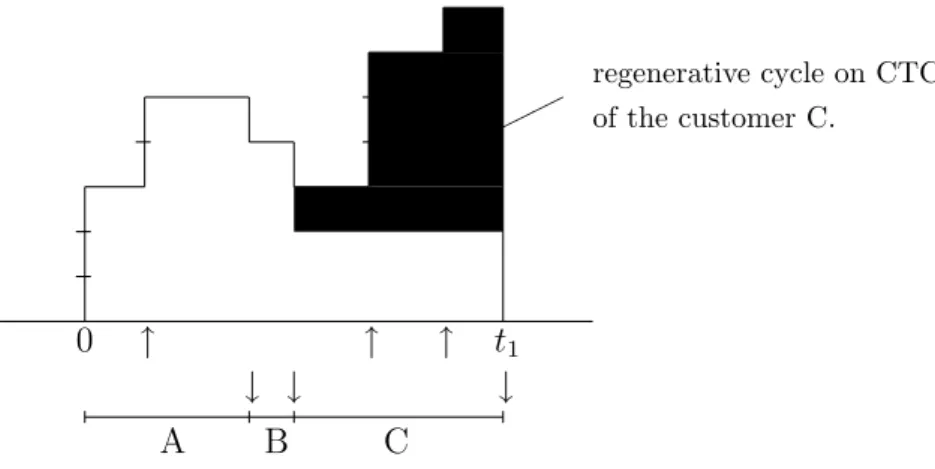
If we try to apply the result in previous section to a concrete model, we must obtain the Π(z : CT ). This is the PGF of the regenerative cycle on the completion time of the batch. In most applications the completion time of the batch consists of the completion times of customers(CTC) belonging to this batch. As an example, in the model MX/G/1 the completion time of a batch consists of the service times of its customers. Figure 1 shows an example of the queue length process in this case. The uparrow and the downarrow mean the arrival of batch and the departure of the customer respectively. There is one batch at 0 which we call the initial batch. This batch has three customers A, B and C and the corresponding service intervals constitute the completion time of this batch.
Figure 1: Regenerative cycle on CT of a batch
©©© regenerative cycle on CTC of the customer C. 0 ↑ ↑ ↑ t1 ↓ ↓ ↓ A B C
This section assumes that each customer belonging to the initial batch also has the completion time denoted by CTC. For space saving we assume that every customer has the identical PGF Π(z : CT C) on his completion time, although the PGF of the model with the different Π(z : CT C)’s is able to be calculated.
Let Cc(x), bCc and Cc∗(s) be the distribution function of CTC, its mean and its LST respectively. The customer occupying the interval CT C leaves the system before or at the end of CT C and other customer is not served on this CTC. Although CTC in Figure 1 is his service time, it may contain the vacation time or the loss interval. Let LC
c(z) be the PGF of the number of batches which arrive on CTC and remain just after the end of this interval. Let lC
c be the mean of LCc(z). We assume that these remaining batches continue to stay until the end of the completion time CT of the initial batch. Moreover we assume that the number of customers belonging to such remaining batch is independent of the service rule on CT C, so that its PGF is G(z). This section assumes that each customer has the same triple:
(Cc∗(s), Π(z : CT C), LCc(z)). (5.1)
Then the PGF Π(z : CT ) on the time interval occupied by the initial batch is represented as follows.
Theorem 5.1. Π(z : CT ) = G(z) − G(LCc(G(z))) g¡z − LC c(G(z)) ¢ Π(z : CT C), |z| < 1, (5.2) C∗(s) = G(C∗ c(s)), bC = bCcg, (5.3) LC(z) = G(LC c(z)), lC = lCcg. (5.4)
Proof. Let’s consider the completion time of an initial batch. Let N be the number of
customers belonging to this batch. When N = n is given, the interval occupied by the initial batch is divided by n completion time intervals CT C1, · · · , CT Cn of customers. At the beginning of CT Ci there are n − i + 1 customers of the initial batch in the system and besides there are the batches arriving on CT C1, · · · , CT Ci−1. The PGF of the number of the batches arriving on Si−1j=1CT Cj and remaining until the end of CT Ci is LCc(z)i−1. Therefore the PGF on CT of the initial batch with n customers is represented by
Π(z : N = n) = z n−1 n n−1 X i=0 ¡ z−1LCc(G(z))¢iΠ(z : CT C) = zn− LCc(G(z))n n(z − LC c(G(z))) Π(z : CT C). Moreover E(CT |N = n) = nbC
c. The (5.2) follows from Lemma 3.1. Next, we get (5.3) from
C∗(s) = E(e−sCT) = ∞ X n=1 E(e−sCT|N = n)P r(N = n) = ∞ X n=1 Cc∗(s)nP r(N = n) = G(Cc∗(s)).
Let H be the number of batches arriving during the completion time of the initial batch and remaining until its end. Then
LC(z) = ∞ X m=0 zmP r(H = m) = ∞ X m=0 ∞ X n=1 zmP r(H = m|N = n)P r(N = n) = ∞ X n=1 LCc(z)nP r(N = n) = G(LCc(z)). 5.2. Π¡z : M/CT /1¢
Applying the results of Theorem 5.1 to the equations of Theorem 4.1, we get the following. Theorem 5.2. Π¡z :busy/M/CT /1¢= (1 − l C cg)(1 − G(z)) g{LC c(G(z)) − z} Π(z : CT C), (5.5) Π¡z : M/CT /1¢= 1 − lCcg 1 − lC cg + λbCcg n 1 + λbCc(1 − G(z)) LC c(G(z)) − z Π(z : CT C) o . (5.6)
When no arriving batch is lost, we get Π¡z :busy/M/CT /1¢= (1 − λb C cg)(1 − G(z)) g(C∗ c(λ − λG(z)) − z) Π(z : CT C), (5.7) Π¡z : M/CT /1¢= (1 − λbC cg) n 1 + λbCc(1 − G(z)) C∗ c(λ − λG(z)) − z Π(z : CT C) o . (5.8)
We can represent various PGF’s by Π(z : CT C), if we substitute these equations to (4.12), (4.13) or their combinations.
Let’s check (5.8) by applying it to MX/G/1. We can put
Cc(x) = B(x), bCc = b and Π(z : CT C) = z
1 − B∗ G(z)
λb(1 − G(z))
where B∗
G(z) = B∗(λ − λG(z)). From (5.8), we obtain the following time average PGF.
Π(z : MX/G/1) = (1 − λgb)(1 − z)BG∗(z)
B∗
G(z) − z
. (5.9)
This is equal to the equation (4.18c) in p.48 of [30].
6. Application to Some Variants of MX/G/1 6.1. One-service-one-vacation rule
Our completion time method is useful not only for the batch arrival but also for the special vacation models. First we will consider the one-service-one-vacation rule which is called the pure limited service system in [30]. In this rule the server takes a vacation immediately after the service of each customer. This section denotes the distribution function of the length of this vacation by V (x). The server begins the first service of the batch at the beginning of its completion time. When the service of each customer is completed, this customer leaves the system and the server takes a vacation. Returning from the vacation, he begins to serve the next customer belonging to the same batch. In this way he repeats the service and the vacation. The end of the completion time is the end of the last vacation in this batch. This section deals with the ordinary vacation and the loss vacation.
The completion time of a customer consists of one service time and subsequent vacation time, so that the PGF Π(z : CT C) is represented as the combination of the PGF on the service period and the PGF on the vacation period. In the case of the ordinary vacation, from (1.1) it has the form:
Π(z : CT C) = α0bz 1 − B∗ G(z) λb(1 − G(z))+ α1vB ∗ G(z) 1 − V∗ G(z) λv(1 − G(z)).
Since α0 = α1 and α0b + α1v = 1, we obtain
Π(z : CT C) = z(1 − BG∗(z)) + BG∗(z)(1 − VG∗(z)) λ(b + v)(1 − G(z)) . (6.1) Moreover C∗ c(s) = B∗(s)V∗(s), bCc = b + v, C∗(s) = G ¡ B∗(s)V∗(s)¢ and bC = g(b + v).
By substituting these to (5.8), we get
Π(z : MX/(G + V )/1) = Π(z : M/CT /1) = (1 − λg(b + v))(1 − z)BG∗(z)
B∗
G(z)VG∗(z) − z
. (6.2)
The (6.2) is the generalization of both (10.6) of [27] and (5.9) of this paper. By substitut-ing (6.2) to the equations in section 4, we can get Π(z : MX/(G + V )/1/N
batch−policy), Π(z :
MX/(G + V )/1/MV (V
1)) and their combinations.
If the batch arriving during the vacation leaves the system immediately without entering it, we call it the loss vacation. The PGF of the regenerative cycle on the loss vacation is Π(z) = 1. In the case that the server takes the loss vacation after the service of each customer, the PGF on the interval occupied by the customer is written by
Π(z : CT C) = αbz 1 − B ∗ G(z) λb(1 − G(z))+ αvB ∗ G(z) = z(1 − BG∗(z)) + λv(1 − G(z))BG∗(z) λ(b + v)(1 − G(z)) . Moreover C∗ c(s) = B∗(s)V∗(s), bCc = b + v, LCc(z) = B∗(λ − λz), lCc = λb. By substituting these results to (5.6) we get
Π(z : MX/(G + V )/1) = Π(z : M/CT /1) = (1 − λbg) © 1 − z + λv(1 − G(z))ªB∗ G(z) (1 + λvg)(B∗ G(z) − z) = 1 1 + λvg n 1 + λv(1 − G(z)) 1 − z o Π(z : MX/G/1). (6.3)
To be interesting, this does not depend on V∗(s) except for v. Moreover this becomes Π(z : M/G/1) when G(z) = z.
6.2. Ordinary customers in the nonpreemptive priority queueing system
In one-service-one-vacation rule the service and the vacation are independent. As an example of the dependent case we will consider the ordinary nonpreemptive priority queues with two classes of customers, i.e., the priority customers and the ordinary customers. Takagi [30] introduced Welch[32]’s doctorial dissertation which obtained the joint distribution of queue lengths of both classes at the every service completion epoch. He says that it is not identical to the PGF of number of messages at an arbitrary time. Takahashi et al.[31] obtained the relation between queue length and the waiting time. This section shows that our completion time method is useful for obtaining the time average PGF of the number of ordinary customers.
Let B(x), b and B∗(s) be the distribution of the service time of the ordinary customer, its mean and its LST respectively. The ordinary customers arrive in batches whose PGF is represented by (2.1). This is the Poisson arrival with intensity λ. Let B1(x), b1 and
B∗
1(s) be the distribution of the service time of the priority customer, its mean and its LST
respectively. This is single and Poisson arrival with intensity λ1. Assume λ1b1+λbg < 1. We
is not interrupted but the new service of ordinary customer cannot start when there is a priority customer.
The priority customers arriving during the service period of the ordinary customer are served after it. Therefore as the completion time CTC of an ordinary customer we choose the time interval from the starting epoch of the service of this customer to the epoch when the server is free to accept the next ordinary customer. The number of the priority customers on this interval is the regenerative cycle of M(λ1)/G(B1)/1/MV (B). Therefore the LST of
our completion time is given by
C∗ c(s) = B∗(s + λ1− λ1Θ∗1(s)), bCc = b 1 − λ1b1 , (6.4) (see [30] p.24) where Θ∗
1(s) is the LST of the busy period in M(λ1)/G(B1)/1. The Θ∗1(s)
satisfies Θ∗
1(s) = B1∗(s + λ1− λ1Θ1∗(s)) from (4.3). We put θ1 = b1/(1 − λ1b1) which is the
mean of this busy period.
We must combine two cases. First, if the ordinary customer finds an idle server at his arrival, the busy cycle of M/CT /1 with our completion time begins. Secondly, if a priority customer finds an idle server at his arrival, the service interval for the priority customers begins. The LST of this length is Θ∗
1(s). Since the ordinary customers may arrive during
this interval, they generate the regenerative cycle of M/CT /1/MV (Θ1). Totally, the PGF
of the number of ordinary customers is represented by
Π(z) = α0 1 λ1+ λ + α1 bC c 1 − λbC c Π¡z :busy/M/CT /1¢+ α2 θ1 1 − λbC c Π¡z :M/CT /1/MV (Θ1)¢. Since α0 : α1 : α2 = 1 : λ/(λ1+ λ) : λ1/(λ1 + λ), we have Π(z) = (1 − λ1b1)Π(z : M/CT /1) + λ1b1Π ¡ z :M/CT /1/M V (Θ1)¢. (6.5) Or by using (4.13) Π(z) = (1 − λ1b1) n 1 + λ1(1 − Θ ∗ 1(λ − λG(z)) λ(1 − G(z)) o Π¡z : M/CT /1¢. (6.6)
Lastly we must calculate Π(z : CT C). Theorem 6.1. Π(z : CT C) = z(1 − BG∗(z)) + BG∗(z) − B∗(λ1− λ1Θ∗1G(z) + λ − λG(z)) λb(1 + λ1θ1)(1 − G(z)) , Π(z : M/CT /1) =¡1 − λbg 1 − λ1b1 ¢ (1 − z)B∗ G(z) B∗(λ 1 − λ1Θ∗1G(z) + λ − λG(z)) − z .
Proof. Our CTC consists of the service period of one ordinary customer and the service
period ΘP of the priority customers. The number of the ordinary customers on the former period is cumulative, so that its PGF is z{1 − B∗
G(z)}/{λb(1 − G(z))}.
Next consider the latter period ΘP. Let N1 be the number of the priority customers
arriving during the former service period. Let N be the number of batches of the ordinary customers arriving during the same period. Then
∞ X
j=0,k=0
When N1 = n1 is given, the LST of the length of ΘP is Θ1∗(s)n1. Its mean is n1θ1.
Therefore when N1 = n1 and N = n are given, the regenerative cycle of the ordinary
customers on ΘP is cumulative and its PGF is
Π¡z :NN =n1=n1¢= G(z)n 1 − Θ ∗ 1G(z)n1 λn1θ1(1 − G(z)) where Θ∗ 1G(z) = Θ∗1(λ − λG(z)). The Mean of ΘP is E(ΘP) = θ1 ∞ X n1=0 n1P r(N1 = n1) = λ1bθ1.
From Lemma 3.1 the PGF of the regenerative cycle on ΘP is given by
Π¡z : ΘP ¢ = 1 E(ΘP) ∞ X n1=0,n=0 P r(N1 = n1, N = n)n1θ1Π ¡ z :NN =n1=n1¢ = B ∗ G(z) − B∗(λ1− λ1Θ∗1G(z) + λ − λG(z)) λλ1bθ1(1 − G(z)) . Consequently from (1.1) Π(z : CT C) = α1b z(1 − B∗ G(z)) λb(1 − G(z)) + α2λ1θ1bΠ ¡ z : ΘP ¢ .
Since α1 = α2 and α1b + α2λ1θ1b = 1, we get the equation of Π(z : CT C).
Substituting this result into (5.8) we complete the proof. 6.3. Time-controlled service system
6.3.1. Service rule and lemma
Some authors([16, 17, 23, 30]) considered the waiting time or unfinished work in the time-limited service system. The term ”time-time-limited” gives us the impression that the service time is limited by the timer. Here more generally we will consider the service rule controlled by the timer and obtain Π(z : CT C) by choosing the completion time adequately. We assume that the timer starts simultaneously with the service. The time T until the timer expiration is independent of the service time. First we do not specialize the distribution of
T .
Let S be the service time of a customer. This section chooses S as the completion time of a customer if S < T . When T ≤ S, we can consider many rules like the priority queues(e.g., [14]). The main rules in this case are as follows.
(1) The server takes the vacation after the service S.
(2) The service is changed at the timer expiration to the new service with the service time S0. The server takes the vacation after S0.
(3) The customer leaves the system at T and the server takes the vacation. (4) The service is interrupted by the vacation.
(4-1) The remaining service is resumed after the vacation. The remaining service does not have the timer.
(4-2) The new service S0 begins after the vacation. This service does not have the
(5) The service is interrupted by the vacation. After the vacation the service begins. Any service has the timer. In this way the service and the vacation repeat alternately until the service ends without timer expiration.
(5-1) After every vacation the remaining service is resumed. That is, the total service time is S.
(5-2) After any vacation the identical service time begins all over again.
(5-3) Whenever the vacation ends, new service with the same distribution as S starts independently.
This section deals with the ordinary vacation, although the loss vacation or loss interval is considerable. We assume that our vacation is independent of the service time.
6.3.2. Rules (1), (2) and (3)
Let’s consider a variant of MX/G/1 in which every customer receives the service according to the identical time-controlled service rule. Here, we will consider Rules (1), (2) and (3) in which the customer leaves the system before the vacation. Let ˜S be the service time which
the customer receives actually. Let BS˜(x), bS˜ and B∗S˜(s) be the distribution function of
˜
S, its mean and its LST respectively. The B∗ ˜
S(s : S < T ) and B ∗ ˜
S(s : T ≤ S) denote the LST of ˜S conditioned by S < T and T ≤ S respectively. If S < T , then ˜S = S. We put p = P r(S < T ). We have B∗ ˜ S(s) = Z ∞ 0 e−sxdP r( ˜S ≤ x) = Z ∞ 0 e−sxdP r( ˜S ≤ x, S ≤ T ) + Z ∞ 0 e−sxdP r( ˜S ≤ x, T < S) = pBS∗˜(s : S < T ) + (1 − p)BS∗˜(s : T ≤ S). (6.7)
The completion time CT C of a customer is
CT C = ½ S : S < T , ˜ S + V : T ≤ S. Therefore C∗ c(s) = Z ∞ 0 e−sxdP r(CT C ≤ x) = Z ∞ 0 e−sxdP r( ˜S ≤ x, S < T ) + Z ∞ 0 e−sxdP r( ˜S + V ≤ x, T ≤ S) = pBS∗˜(s : S < T ) + (1 − p)BS∗˜(s : T ≤ S)V∗(s), (6.8) bCc = bS˜+ v(1 − p). (6.9) We put B∗ ˜ SG(z) = B ∗ ˜ S(λ − λG(z)), B ∗ ˜ SG(z : S < T ) = B ∗ ˜ S(λ − λG(z) : S < T ), B∗ ˜ SG(z : T ≤ S) = BS∗˜(λ − λG(z) : T ≤ S) and CcG∗ (z) = Cc∗(λ − λG(z)). Theorem 6.2. In Rules (1), (2) and (3)
Π(z : CT C) = z{1 − B ∗ ˜ SG(z)} + B ∗ ˜ SG(z) − C ∗ cG(z) λbC c(1 − G(z)) , Π(z : M/CT /1) = (1 − λb C cg)(1 − z)BSG∗˜ (z) C∗ cG(z) − z .
Proof. In these rules the regenerative cycle on CT C consists of the cumulative process on
˜
S and the cumulative process on V . Therefore
Π(z : CT C) = α1bS˜ z{1 − B∗ ˜ SG(z)} λbS˜(1 − G(z)) + α2vΠ l(z) 1 − VG∗(z) λv(1 − G(z)).
The Πl(z) is the PGF of the number of customers arriving during the service time under the condition T ≤ S, so that Πl(z) = B∗
˜
SG(z : T ≤ S). Moreover, α1 : α2 = 1 : 1 − p and
α1bS˜+ α2v = 1, so that we have α1 = 1/bCc and α2 = (1 − p)/bCc. Consequently we get
Π(z : CT C) = z{1 − B ∗ ˜ SG(z)} + (1 − p)B ∗ ˜ SG(z : T ≤ S){1 − V ∗ G(z)} λbC c(1 − G(z)) .
From (6.7) we get Π(z : CT C) in the theorem. By substituting it to (5.8) we get the theorem.
We can also obtain Π¡z :M/CT /1/Npolicy ¢of (4.11), Π¡z :M/CT /1/MV (V1)¢of (4.12) and these combinations from this result.
6.3.3. Rules (4) and (5)
In Rules (4) and (5) the completion time of a customer begins simultaneously with his service and ends at his departure, so that Π(z : CT C) is the PGF of the cumulative process on CTC. Completion times of Rules (4-1) and (4-2) are the same as those of Rules (1) and (2) respectively. When in Rule (5-1) one service is interrupted by n vacations, the completion time CT C is represented by
CT C = S + V1+ · · · + Vn.
If T is distributed exponentially with mean 1/ζ, this form is similar to the busy time of
M/G/1. Therefore C∗
c(s) = B∗(s + ζ − ζV∗(s)), bCc = b(1 + ζv). (6.10) The (6.10) is substantially the same as (2.13) of [14]. Similarly we find C∗
c(s) about Rules (5-2) and (5-3)(see [10]).
We get the following theorem. Theorem 6.3. In Rules (4) and (5)
Π(z : CT C) = z(1 − C ∗ cG(z)) λbC c(1 − G(z)) , Π(z : M/CT /1) = (1 − λbCcg)(1 − z)CcG∗ (z) C∗ cG(z) − z . 6.3.4. B∗ ˜ S(s), b C c and Cc∗(s)
In applying Theorems 6.2 and 6.3 to Rules (1), (2), (3) and (4) we need B∗ ˜ S(s), C
∗
c(s) and
bS˜. Therefore we need to obtain BS∗˜(s : S < T ) and BS∗˜(s : T ≤ S). The previous authors
considered the exponential distribution about T . When T starts before the service, the exponential distribution is useful and even necessary. We will show that, if T starts simul-taneously with the service, we can obtain these conditional LST’s for Erlang distribution of
T . Assume that Ti(i = 1, 2, · · · ) is exponentially distributed with mean 1/ζ. We put
pn = P r ³Xn i=1 Ti ≤ S < n+1 X i=1 Ti ´ , qn= P r ³Xn i=1 Ti ≤ S ´ = ∞ X i=n pi.
Since the PGF of pn is given by P∞
n=0znpn = B∗(ζ − ζz), we have pn= (−ζ)nB∗(n)(ζ). We use the following theorem.
Theorem 6.4. (i) The LST of S conditioned by Pni=1Ti ≤ S < Pn+1
i=1 Ti is
B∗(n)(s + ζ)/{n!B∗(n)(ζ)}.
(ii) The LST’s of S conditioned by Pni=1Ti ≤ S or S < Pn
i=1Ti are respectively 1 qn n B∗(s) − n−1 X j=0 (−ζ)j j! B ∗(j)(s + ζ)o and 1 1 − qn n−1 X j=0 (−ζ)j j! B ∗(j)(s + ζ).
(iii) The LST of Pni=1Ti conditioned by Pn i=1Ti ≤ S is ³ ζ s + ζ ´n1 qn n 1 − n−1 X i=0 (−s − ζ)i i! B ∗(i)(s + ζ)o.
Proof. (i) We denote the conditional distribution function of (i) by F (x) = 1 pn P r ³ S ≤ x, n X i=1 Ti ≤ S < n+1 X i=1 Ti ´ . Since P r ³ S ≤ x, n X i=1 Ti ≤ S < n+1 X i=1 Ti ´ = Z x 0 (ζs)n n! e −ζsdB(s),
from the formula of variable transformation(see [12][13]) the LST of F (x) is
F∗(s) = Z ∞ 0 e−sxdF (x) = 1 pn Z ∞ 0 e−sx(ζx)n n! e −ζxdB(x) = 1 B∗(n)(ζ) Z ∞ 0 (−x)n n! e −(s+ζ)xdB(x) = B∗(n)(s + ζ) n!B∗(n)(ζ) . (ii) We put F (x) = P r(S ≤ x, Pn i=1Ti ≤ S) P r(Pni=1Ti ≤ S) = 1 qn n P r(S ≤ x) − n−1 X j=0 P r ³ S ≤ x, j X i=1 Ti ≤ S < j+1 X i=1 Ti ´o .
Hence the first half of (ii) follows from (i). Similarly we find the second half. (iii) We put F (x) = P r( Pn i=1Ti ≤ x, Pn i=1Ti ≤ S) P r(Pni=1Ti ≤ S) = 1 qn Z x 0 P r(t ≤ S) ζ ntn−1 (n − 1)!e −ζtdt = 1 qn Z x 0 (1 − B(t)) ζ ntn−1 (n − 1)!e −ζtdt. Hence F∗(s) = Z ∞ 0 e−sxdF (x) =³ ζ s + ζ ´n 1 qn Z ∞ 0 (1 − B(x))(s + ζ)n (n − 1)!x n−1e−(s+ζ)xdx. (6.11)
Since the function f (x) = 1 − n−1 X i=0 {(s + ζ)x}i i! e −(s+ζ)x satisfies f (0) = 0, f0(x) = (s + ζ) n (n − 1)!x n−1e−(s+ζ)x,
by the integration by parts(see [12][13]), (6.11) becomes
F∗(s) =³ ζ s + ζ ´n 1 qn Z ∞ 0 n 1 − n−1 X i=0 {(s + ζ)x}i i! e −(s+ζ)xodB(x) =³ ζ s + ζ ´n 1 qn n 1 − n−1 X i=0 (−s − ζ)i i! B ∗(i)(s + ζ)o.
Assume that T has the k−Erlang distribution. We represent it such as T =Pki=1Ti by using Ti in Theorem 6.4. Then we get from (ii) of this theorem
B∗ ˜ S(s : S < T ) = 1 1 − qk k−1 X j=0 (−ζ)j j! B ∗(j)(s + ζ) (6.12)
for all our rules, because ˜S = S under this condition.
In Rules (1) and (4-1) we have ˜S = S, so that bS˜ = b and BS∗˜(s) = B∗(s). From (ii) of
Theorem 6.4 C∗ c(s) in (6.8) becomes Cc∗(s) = k−1 X j=0 (−ζ)j j! B ∗(j)(s + ζ) +nB∗(s) − k−1 X j=0 (−ζ)j j! B ∗(j)(s + ζ)oV∗(s) (6.13) and bC c = b + vqk. In Rule (3) we have B∗ ˜ S(s) = k−1 X j=0 (−ζ)j j! B ∗(j)(s + ζ) +³ ζ s + ζ ´kn 1 − k−1 X j=0 (−s − ζ)j j! B ∗(j)(s + ζ)o (6.14)
from (iii) of Theorem 6.4 and (6.7). Similarly we get bC
c and Cc∗(s). In the same way we can obtain such values for Rules (2) and (4-2).
6.4. Preemptive priority queueing system with a timer
Let’s apply the results of the previous sections to the ordinary customers in the preemptive priority queueing systems. The notations λ, B(x), b, B∗(s), B
1(x), b1, B1∗(s) and G(z)
are the same as section 6.2.
In the pure preemtive rule the priority customer begins to receive the service at his arrival, if there is no other priority customer. Hence the LST of the distribution of the length of the service period of priority customers is given by Θ∗
1(s) of (6.4). If we regard
this period as the vacation and put ζ = λ, we can obtain the PGF of the number of the ordinary customers in the priority rules corresponding (4) and (5) in section 6.3.
Katayama[18] considered the nonpreemptive queueing system with a timer control. His model is inconvenient for our completion method. Here we assume that the timer T starts at the beginning of the service S of the ordinary customer. If S < T , the S is not interrupted and the priority customers are served immediately after this. If T < S, the S is interrupted at the expiration of T . At once the priority customers, if any, begin to receive the services. We can consider the following two cases.
(i) The interrupted ordinary customer leaves the system regardless of the existence of the priority customer.
(ii) The interrupted ordinary customer waits for the end of the services of the priority customers and then receives the new service S0. S0 is independent of the first service.
In these rules there is no priority customers at the beginning of the service of the ordinary customer. Therefore as the completion time of an ordinary customer we choose the time interval from the starting epoch of the service S of this customer to the epoch when the server is free to accept the next ordinary customer. In rule (i) the actual service time ˜S of
the ordinary customer is ˜S = S if S < T , and ˜S = T if T ≤ S. Hence we can obtain its LST B∗ ˜ S(s) from (6.7), if we get B ∗ ˜ S(s : S < T ) and B ∗ ˜
S(s : T ≤ S). When T has the k−Erlang distribution, B∗
˜
S(s) is given by (6.14). Since the interrupted ordinary customer leaves at once, the rule (i) is essentially equivalent to the nonpreemptive priority rule. That is, if we represent the PGF of Theorem 6.1 as Π(z : CT C, B∗(s)), the PGF of the regenerative cycle of the ordinary customers on the CTC in this section is represented by
Π ³ z : CT C, B∗ ˜ S(s) ´ .
Similarly we can obtain the Π(z : CT C) also for the rule (ii), whether S0 has a timer or
not. However we will omit it for the complexity of the calculation.
7. Probabilities and Moments
Our results (5.9), (6.2), Theorem 6.1, Theorem 6.2 and Theorem 6.3 about M/CT /1 have the form
Π(z) = a(1 − z)A(z)
K(z) − z ,
where A(1) = 1 and a = 1 − K0(1). We can calculate probabilities and moments for such PGF by the method of [27]. That is, we obtain the following recursive equations.
Π(n)(0) = 1 K(0) n − n−1 X i=0 µ n i 
K(n−i)(0)Π(i)(0) + nΠ(n−1)(0) − naA(n−1)(0) + aA(n)(0) o , Π(n)(1) = 1 (n + 1)(1 − K0(1)) n−1 X i=0 µ n + 1 i ¶ K(n+1−i)(1)Π(i)(1) + An(1).
For example, the moments of one-service-one-vacation model (6.2) are obtained by the recursive equation Π(n)(1) = 1 (n + 1)(1 − ρ) n−1 X i=0 n+1−iX j=0 µ n + 1 i ¶µ n + 1 − i j ¶ B∗(n+1−i−j)G (1)VG∗(j)(1)Π(i)(1) + BG∗(n)(1),
where ρ = λg(b+v). For some models, choosing Erlang distributions for service and vacation, the author checked these moments for various parameter values by computer simulation.
References
[1] Y. Baba: On the MX/G/1 queue with vacation time. Operations Research Letters, 5 (1986), 93–98.
[2] P.J. Burke: The output of a queueing system. Operations Research, 4 (1956), 699–704. [3] M.L. Chaudhry: The queueing system MX/G/1 and its ramifications. Naval Research
Logistics Quartary, 26 (1979), 667–674.
[4] M.L. Chaudhry and J.G.C. Templeton: A First Course in Bulk Queues (John Wiley & Sons, New York, 1983).
[5] G. Choudhury: An MX/G/1 queueing system with a setup period and a vacation period. Queueing Systems, 36 (2000), 23–38.
[6] J.W. Cohen: The Single Server Queue (North-Holland, New York, 1982).
[7] D.R. Cox: The analysis of non-Markovian stochastic processes by the inclusion of supplementary variables. Proceeding of Cambridge Philosophical Society, 51 (1955), 433–441.
[8] S.W. Fuhrmann and R.B. Cooper: Stochastic decompositions in the M/G/1 queues with generalized vacations. Operations Research, 33 (1985), 1117–1129.
[9] D.P. Gaver, Jr.: Imbedded Markov chain analysis of a waiting-line process in continuous time. Annals of Mathematical Statistics, 30 (1959), 698–720.
[10] D.P. Gaver, Jr.: A waiting line with interrupted service, including priorities. Journal
of the Royal Statistical Society, Series B, 24 (1962), 73–90.
[11] D. Gross and C.M. Harris: Fundamentals of Queueing Theory (John Wiley & Sons, New York, 1974).
[12] P.R. Halmos: Measure Theory (Springer-Verlag, New York, 1974).
[13] S. Itou: Lebesgue sekibunn Nyuumon (Mokabou, Tokyo, 1958)(In Japanese). [14] N.K. Jaiswal: Priority Queues (Academic Press, New York, 1968).
[15] U. Kal¨ahne: Existence, uniqueness and some invariance properties of stationary distri-butions for general single-server queues. Optimization, 7 (1976), 557–575.
[16] T. Katayama: Waiting time analysis for a queueing system with time-limited service and exponential timer. Naval Research Logistics, 48 (2001), 638–651.
[17] T. Katayama: Level-crossing approach to a time-limited service system with two types of vacations. Operations Research Letters, 33 (2005), 295–300.
[18] T. Katayama: Analysis of a time-limited service priority queueing system with expo-nential timer and server vacations. Queueing Systems, 57 (2007), 169–178.
[19] D.G. Kendall: Some problems in the theory of queues. Journal of the Royal Statistical
Society, Series B, 13 (1951), 151–185.
[20] D.G. Kendall: Stochastic processes occurring in the theory of queues and their analysis by means of the imbedded Markov chain. The Annals of Mathematical Statistics, 24 (1953), 338–354.
[21] H.W. Lee, S.S. Lee, and K.C. Chae: Operating characteristics of MX/G/1 queue with
N-policy. Queueing Systems, 15 (1994), 387–399.
[22] H.W. Lee, S.S. Lee, J.O. Park, and K.C. Chae: Analysis of the MX/G/1 queue with
N-policy and multiple vacation. Journal of Applied Probability, 31 (1994), 476–496.
[23] K.K. Leung and M. Eisenberg: A single-server queue with vacations and non-gated time-limited service. Performance Evaluation, 12 (1991), 115–125.
[24] J. Loris-Teghem: On vacation models with bulk arrivals. Belgian Journal of Operations
Research, Statistics and Computer Science, 30-1 (1990), 54–66.
[25] J. Loris-Teghem: Remark on on vacation models with bulk arrivals. Belgian Journal of
Operations Research, Statistics and Computer Science, 30-4 (1990), 54–56.
[26] T. Nakatsuka: Absorbing process in recursive stochastic equations. Journal of Applied
Probability, 35 (1998), 418–426.
[27] T. Nakatsuka: The regenerative cycle method in M/G/1 with many vacation rules.
Journal of the Operations Research Society of Japan, 46 (2003), 503–522.
[28] L. Tak´acs: The transient behavior of a single server queueing process with a Poisson input. Proceedings of the Fourth Berkeley Symposium on Mathematical Statistics and
Probability, 2 (1961), 535–567.
[29] L. Tak´acs: Introduction to the Theory of Queues (Greenwood Press, Westport, 1962). [30] H. Takagi: Queueing Analysis, Volume 1:Vacation and Priority Systems, Part 1
(North-Holland, New York, 1991).
[31] Y. Takahashi and M. Miyazawa: Relationship between queue-length and waiting time distributions in a priority queue with batch arrival. Journal of the Operations Research
Society of Japan, 37 (1994), 48–63.
[32] P. D. Welch: Some contributions to the theory of priority queues. Ph.D. Thesis, Depart-ment of Mathematical Statistics, Columbia University; IBM Research Report RC-922, IBM Research Center, Yorktown Heights, New York.
[33] R. W. Wolff: Stochastic Modeling and the Theory of Queues (Prentice-Hall, Englewood Cliffs, 1989).
Toshinao Nakatsuka
Faculty of Urban Liberal Arts Tokyo Metropolitan University
1-1 Hachiouji-shi, Tokyo 192-0397, Japan E-mail: [email protected]