Variable Separation Principle for Mathematical Programming

(1)

VARIABLE SEPARATION PRINCIPLE FOR

MATHEMATICAL PROGRAMMING

IW ARO TAKAHASHI Waseda University, Tokyo

(Received Feb. 4, 1963)

§ 1. THE CONCEPT OF VARIABLE SEPARATION PRINCIPLE

fhe ploblem of mathematical programming IS to maximize (or

minimize) a objective functionf(x) subject to constraints, which are usually expressed as gi(X)=O (or gi(X)~O), i= 1,2, ...

We classify these constraints into two types; simple and complicating. Simple constraints are such as Xi~O, Mi~Xi~O, etc., while let us call such constraints complicating, that complicate the problem because of involving many variables. In other words, if there were no complicating constraints, variables would be separated into several groups and we could treat the problem separately for each group.

Lagrange function is the sum of objective function and constraint functions weighted with Lagrange multipliers. Kuhn & Tucker (XII) show-ed the equivalence of mathematical programming and minimax problem of the Lagrange function.

The basic ideas of Variable Separation Principle are as follows; (a) Select complicating constraints out of given constraints, and take only complicating constraints into the Lagrange function.

(b) Optimize the Lagrange function in x (constrained with simple

constraints) with Lagrange multipliers fixed. In this process we can treat variables separately, with appropriately selected complicating constraints. (c) Next modify the Lagrange multipliers so that complicating constraints are satisfied.

In step (b) the optimal value of the objective function is a func-tion of Lagrange multipliers A

=

(}'1' ... , Am) which we denote L().).

82

(2)

Variable Separation Principle for Mathematical Programming 83

In this paper, we clarify the properties of L(A) and make general

algorithms for process (c).

The effectiveness of our principle in application depends on the selection to select complicating constraints. We show examples of applica-tion of our principle in § 5,6, 7, and 8.

§ 2. BELLMAN SURF ACE B(y) AND LEGENDRE

FUNCTION L(A)

Let us consider X=(Xl,"" Xm) and its objective function ((x) and

constraint functions gi(X) (i= I~m). Besides gi(X)=O (i= I~m) there may be constraints for x, the domain restricted with which we denote C. gi(X)=O (i= l~m) are correspond to complicating constraints and C is

correspond to simple ones.

The maximum value of f(x) subject to gi(X) = Yi (i= I~m) and XEC

is a function of Y=(Yl' ... , YIn), so we denote it B= B(y). That is,

(1) B=B(y)=Max {f(X)! gi(X) =Yi (i=: I~m)}

XEC

we call it Bellman surface, (being sugg;sted by (Ill) (IV».

The maximum value of Lagrange function f(X)+A1g1(X)+"'+Amgm(X)

in _{xEC with A=(J.1, ... , Am) fixed,} is a function of A, so we denote it L=L(A). That is

(2) L=L(A)=Max {f(XHA1g1(xH .. ·--!-J.mgm(X)} xEC

We call it Legendre function. (Theorem 1)

If

{

f(x) is a convex* function, gi(X) are linear functions (i= I-m)

(3)

and C is a convex set, then B(y) is a convex function.

Furthermore if f(x) is strictly convex,* then B(y) is strictly convex.

*

If F(Ox+(l-O)y);;;;OF(x)+(l-O)F(y) (O~O~l), we call F(x) convex function, and if ;;;:; is replaced

by>,

strictly convex.

(3)

Iwaro Takahashi

Let us assume that the conditions (3) are satisfied throughout this paper.

Let ~!o " ' , ~m' tjJ be Cartesian coordinates of

(m+

1) dimensional

space.

expresses a surface K in this space. (Point expression of surface). Consider

a supporting plane of K whose normal cosines are proportional to

(7] I, .•• , 7]m, I)

which we denote n(7]I, ..• , 7]m). The value IJf' of tjJ-coordinate of the

cross point of tjJ-axis and n(7]I'"'' 7]m) is the function of 7]=(7]1'"'' 7]m) so

denote it

(5) IJf' =G (7]1'''', 7]m)

Conversely, given (5), a plane whose normal cosines are proportional to (7]1;"" 7]m, 1) and which crosses tjJ-axis at IJf' =G (7]1'"'' 7]m) is uniquely

determined in tjJ-~ space. The envelope of such planes is the surface K.

That is, (5) is another expression of K (supporting plane expression of

surface), and G is called Legendre Transform of F (CV), (VII». (Fig. 1).

If F is convex, n(7]I,"" 7]m) is uniquely determined for an 7]=(7]1"'" 7]m), and ~-coordinates of contact points are called points (of~)

Legendre-mapped (or simply L-Legendre-mapped) from an 7]. If F is strictly convex, there

is only one point L-mapped from an 7]. But generally more than one

points may be L-mapped from an 7], and a set of these points is a convex

set. (Fig. 1). One point of ~ may be simultaneously L-mapped from 7]1

and 7]2 (7]1~7]2). n(7]I,"" 7]m) is a supporting plane of K at points L-mapped

from 7].

In the case that if ~i is a point L-mapped from 7]i(i= 1, 2) and

7]1~7]2 then ';-1 allways different from

e,

a supporting plane of

K

at a ~

is uniquely determined and coincides with a tangent plane.

Furthermore if (5) is the point expression of

K'

in 7]-1Jf' space, its

(4)

normal).

So (4) is the Legendre Transform of (5). (Theorem 2)

L(A) is Legendre Transform of B(y), so L(A) is concave.

Let

y

be any point L-mapped from A, then

(6) L(A)=B(y)+AY

K ,

}<'ig. 1. Legendre Transform

§ 3.

USE OF

L(A)

FOR MATHEMATICAL

PROGRAMMING

Let us consider a mathematical programming with equality

con-straints for gi(X);

(1) Max f(x) Sub gi(X)=O (i= I-m), XEC

Strictly convex case

First consider the case where f(x) and B(y) are strictly convex. In

this case x maximizing § 2 (2) is uniquely determined, so y L-mapped

from a A is uniquely determined, and the next theorem holds.

(Theorem 1)

(5)

lwaro Takahashi

0=(0, ... , 0)

Conversely A L-mapped from a y=O is A*, and B(O)=L(A*)

Further, x maximizing § 2 (2) for A=A* is the optimal solution or (I).

General Case

Next consider the case where f(x) and B(y) are not necessarily

strictly conxex. (Theorem 2)

Let A* be a minimum point of L(A), then the set of points

L-mapp-ed from A* contains 0=(0, ... , 0), and B(O)=L(A*)

Furthermore x which maximizes § 2 (2) for A=A* and satisfies gi(X)=O is a optimal solution of (I).

(Corollary)

If (I) is nonfeasible, then the minimum value of L(A) is not finite. Numerical example of a mathematical programming, B(y) and L(A)

Consider a mathematical programming;

Let Max 3Xl +4xz sub ,'Xl +xz;;;;;3 :2Xl+Xz=2

lXi~O

(i

=

I, 2) f(x) =3Xl+ 4xz, C=Jxl+xz;;;;;3 g(x)=2-2xl-XZ' lXi~O (i= I, 2) B(y)=Max {3Xl+4xzI2-2xl-XZ=Y} XEC

is shown in Fig. 2 (a). (Values of B do not exist for y>2, y< -4). L(A)=Max {3Xl+4x2+A (2-2xl-X2)}

XEC

(6)

Variable SeparatiQn Principle fQr Mathematical PrQgramming 87 B \ L

\t

14

12

10 8

6

4

2

(a)

-4

-2

o

Cb)

2

y -L---L--~2--~4----6~--

-2

0

A

Fig. 2. B(y) and L().).

§ 4. MINIMUM SEARCH OF L(),)

Strictly convex case (local approach)

Here we explain the successive approximation method to search for a minimum point of L()') in the case where f(x) and B(y) are strictly convex. For this the next theorem is important, which is an immediate consequence of the properties of Legendre Transform.

(Theorem 1)

If B(y) is strictly convex, y L-mapped fnm a ), is uniquely deter-mined, so derivatives of L()') exist and

This theorem means that even if we do not know the explicit form of L(),), we can know the differential coefficients of Le),) for a given )"

(7)

88 Iwaro Takahashi

This leads us to the following algorithm;

Initial Step

Chose any AD for a initial point.

Iterative Step

( i) Let x maximizing § 2 (2) for A =A> be x'.

(ii) Compute

(2) Yi'=gi(X') (i= l-m),

and if Yi'=O (i== l-m) then x' IS the optimal solution of § 3 (1) (§ 3

Theorem 1). Otherwise go to (iii). (iii) Compute

and go back to (i).

From (1), (3) we know above algorithm is Gradient method (I)

itself. So for sufficiently small h the convergence has been proved with

concavity of L(A). We call this method local' approch.

General case (Global Approach)

In the case where B(y) is not necessarily strictly convex, the next

theorem corresponds to theorem l.

(Theorem 2)

Y=(Yl'''.' Ym) L-mapped from a A is y-coordinate of

(4) (Yl> ... , Ym, -1)

which are propotional to normal cosines of a supporting plane of L(A)

at the A.

Generally a supporting plane of L(A) at a A is not uniquely

deter-mined, so (3) cannot be used for this case. So we propose another method for minimum search. The basic ideas of this method, which are similar to the cutting plane method (XIII), are as follows;

Chose m+ 1 points AD, •.• , Am such that the roof* of It' (:;=O-m) has

*

The roof of n planes L=ai+ail,ll+···+aim,lm (i=1-1l) is the function (or surface) Max(ai +ail,l,

+ ...

+aim,lm).

(8)

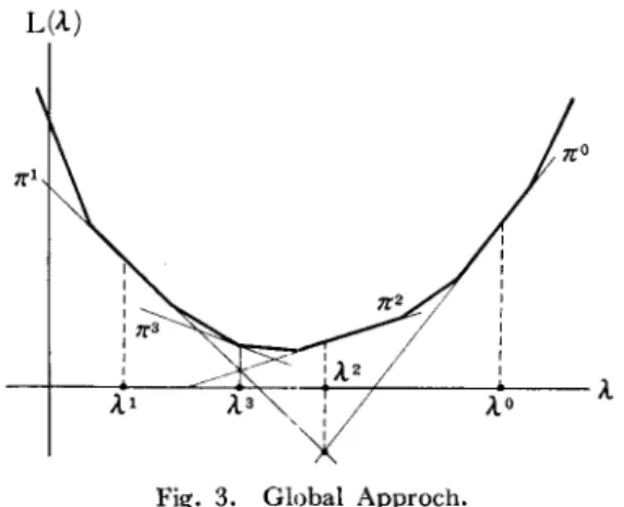
:l finite minimum value, where 11:' is a supporting plane of L(A) at A. Next find the minimum point ).",+1 of the roof. Let 11:",+2 be a support-ing plane of L()') at ).m+l, and find the minimum point Am+2 of the roof

of 11:' (IJ=O-m+ 1), and so on (Fig. 3). Then as N--H>O, AN approches a minimum point of L().). Further, lf L()') is piece-wise linear (like the numerical example of § 3), a finite number of iterations suffice.

We call this method global aP/Jroac/z.

L(,t)

Fig. 3. Global Approch.

Now we describe a theorem by which we concrete above ideas into an algorithm.

(Theorem 3)

Let 11:' be a supporting plane of L()') at k, and normal cosines of 11:' be proportional to (YI', ... , y",',-l) (IJ=O-m). If

.;';;;:;0

satisfying (5) .;0+';2+ ... +.;m=1

';°Yio+';lyil+ ... +.;mYim=O (i= l~'m)

exist, then the roof* of 11:'(IJ=O-m) has finite mmlmum value.

We combine above theorem and the ideas of revised simplex me-thod into the following algorithm;

(9)

90 Iwaro Takaha8hi Initial Step

(i) Choose).' (l.I=O-m) so that Y' L-mapped from )., (l.I=O-m).

satisfy (5). Compute B', L' for k (I.I=O-m).

(6)

(ii) Invert the coefficient matrix of (5).

...

1

i

y~1

y1l ••• y1'ln LY1:LO

y:n

1 _{... y",}In

Iterative Step (i) Compute

=

I ~o I ~1 I : L ::Om ~ ~OI

...

~mo toll

...

tolm ~ ~ ~~1

..

, ';'mm. (7) {lm+1=BD~o+Bl~I+"'+Bm~m ).jm+l= -(BD~Oj+Blej+ .. ·+B"'~mj) (j=I-m)

;(",+1

=

(Al",+I, ... , Am"'+I) is a new point. 1m+1 is a minimum value of the roof of 7[' (l.I=O-m).

(ii) Find ym+1 L-mapped from ;(m+1, and compute Bm+1, Lm+1.

Then ;(m+l is a minimum point. Otherwise go to (iii). (iii) Compute

and take

;:"",+1

into i-th element of (m+ I)-th column of (6), then result-ing matrix is (m+l)x(m+2). Let io be a number i which attains (10) Min ~i/;i,m+1 (~i,m+1>O)

i

Sweep out the above (m+I)x(m+2) matrix with pivot~iO, m+1, then delete the (m+ I)-th column. Take number m+ 1 for io' Then return to (i).

Through above stop following relation, holds; (11) Min (LO, ... , LmY~Min L().r~lm+l.

(11) is usefull to determine the range of Min L(A) when we stop the com-putation half-way.

(10)

General algorithm to find initial points was not stated, which we must device for individual examples.

§ 5. LINEAR PROGRAM OF BLOOK DIAGONAL TYPE

Consider linear programs with constraints shown in the following diagram. (VI) A

I

=0

~~J

-0

1 c

1-0

L

D

I~O

If we select the constraints of D part as complicating, then variables are separated into A, B, C part. In this case lex) is not strictly convex so we use global approch.

We trace the process along the next example;

Two groups of variables

x)}\ x;r

are respectively subject to the following transportation type equality constraints and xg)~O, xg)~O ;

x(1) 11 XCl) 12 XCl) 13

12

X(2) 11 xi~) X(2) 13

35

(1) X(ll 21 x(1) 22 xH)

15

X(2) 21 xg) x~f)

-7

10 10

27

I

20

25

30

I Cost coefficient _c(k) i j are C~ll 'J C(2) '1 ---."'----~ - ~---~---2

3

2

3

4

i

(2)

2

4 6

3

6 8

(11)

92 lwaro TakahaBhi

Further

x;f xW

are subject to another constraint (3) g (x) =720-

L:kL:iL:i

aWx;~)=O, where aCll 'J a CZ ) 'J 3 5

7

6

7

8

(4)

I

4 6

7

I 8 8 8 We want to maximize (5)

_Jex)=-

L:kL:iL:i

cW

X Ck ) ij • The coefficients C' of (6)

- {j(XHAg(X)}

can be written as

1+3A 2+5A 3+7A

_i

I

2+6A

(7)

2+4A 4+6A 6+7A

_{1_!:-_8A}

--~---.,-.

~--~---3+7A 4+8A

6+8A 8+8A

--~-.----~~--~

Under the condition with A fixed, we have only to solve separately two transportation problems with cost coefficients (7) and constraints (1).

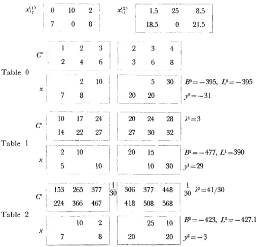
Initial Step

( i) Let AO =0 (arbitrary value of A), and find xO, yO, J!l, LO (Table 0). yO is negative so Al must be a positive lage value, but from (7) we know A1=3 suffice. For A1=3 find xi,yt, Bt, Lt (Table 1).

(ii) Invert

IJ-[ I

y1

-31

into ;Ol

J

=

[29/6()

;11

31/60

2~J

-l/60J

1/60

(12)

Variable Separation Principle for Mathematical Programming 93 Iterative Step ( i ) -395 @ 29/60 --- 1/60 -477

CD

31/60 1/60 -437.2 -41/30

b=-437.2

,(2= 41/30

(ii) Find ~2,y2, E2, L2 for ,]2==41/30 (Table 2).

-3

(iii) ~-,--. --

-I

@ 29/60 -1/60 (32/60)

CD

31/60 1/60 _I 29/60

1

Sweep Out (with

, _ _ _ _ _ _ _ _ _ _ _ 1 _{pivot (}

»

29/32 -1/32 3/32 1/31 -_._---~ ~---( i' ) -423 @ 29/32 --1/32 I La=-428.l -477

_CD

3/32 1/32 _I )..3=27/16 -428.1 -27/16

(ii') Find x3,y3,lP,L3 for )..3:=:27/16 (Table 3).

(iii')

( i" )

1 17

@ 29/32 -1/32 12/32

- - - ---

--,

CD

3/32 1/32 (20/32)

1

Sweep Out (with

pivot (

»

@ 1-17/20 - -1/20

®

1_

3/20 _1/20 __ -423 @ 1-17

/20-~~l/2()1

-453

®I

3/20 1/20! -427.5 --3/2

b=-427.5

)..4=3/2

(13)

so ,<4=3/2 is a minimum point.

Final Treatment

If in the final Table x;~) are unique, then this is the optimal solu-tion (§ 3 Theorem 2). Otherwise, we can choose optimal x;~) out of un-determined x;~) in final Table (§ 3 Theorem 2). That is;

x;;)

circled in in Table 4 are determined by 6xi[l

+

8xW

+

8xW

+

8xa) =397 and constraints

(1). The results are

Table 0 Table 1 Table 2

C'

x

o

10 2

7

2

7 o

2 4 2 8 8 3 I I 6 i I 10

1--i 1---1.5 I 1 18.5 I_~ 2 3 3 6 5 20 20 25

o

4 8 30 8.5 21.5 BO=-395, LO=-395 yO= -31 ___ - I 1 _ _ _ _ _ _ _ _ 10 17 C' I x 14 22 2 5 10 I 153 265 377 13

1 _°1

C' I 1 I

2~~~~

__

~~J

10 2

x

7

8 20 24 28 ,(1=3 27 30 32 ---~-- - -- - - , 20 15 10 30 f=29 306 377 418 508 25 20

448~1 3~

,(2=41/30 568 I 10 .82=-423, L2=-427.1 20

y2=-3

(14)

Variable Separation Principle for Mathematical Programming 95 97 167 237 I 1 194 237 280 1 C' ! 116 16 ;'.3=27/16 140 ! I ₂₂₆ ₂₈₅ _i ₂₆₄ ₃₁₂ ₃₄₄ I Table 3

_-,

-10~~----1

B3=-453, £3=-428.1 10 2 x

8

-11 19 27 C' 16 26 23 Table 4 - - - - -lO 2 x 7 8 " 1

;--22

2, 30 30 i y3=17 27

-S2---IJ

..l4=3/2 36 40, I j - - - -CID 25 CID 'B4=-438, D=-427.5 (y4=7) § 6. RESOURCE ALLOCATION

Let us call the following problem Resource Allocation;

m n

(1) f(x)

= -

E E

CijXij - - > Max. i=1 j=1

n

(2)

E

Xij=ai (i= I-m) (ai~O)

j=1

(4) Xij~O (i=l-m, j=l-n)

We select (2) as complicating. Let

(5) gi(x)=ai- r,Xij (i= I-m) j=l

n

= -

E

{(Clj+A1)Xu+"'+(C,,,;+Am')Xmj} +A1a1 +"'+Amam

j=1

In maximizing (6) subject to (3) (4), we can treat variables separately for each j. For each j, let /j be a ~;et of number

i

attaining

(15)

then Xij satisfying (8) maximize (6);

and maximum value of L()') is

(We need not express L()') explicitly for our pourpose. But by (9) we

know L()') is a piece-wise linear concave function).

We must use global approach to for search a minimum of L(A).

Let us treat the following example:

4 6 7 5 3 17 Initial Step

2

3

2 4 9 15

(i) Let Alo=O, A2o=0, and maximize (6) for ).=AO. For this purpose we have only to write down the Table typed (7), circle the minimum in

each column, and fill up the entries corresponding to circles in x Table

(Table AO).

YIO is negative so we choose a large positive value as All, 6 will

suffice. So let ).11=6, A21_{=0, and maximize (6) for A=AII. By the same}

procedure, we get Table AI. Next choose AI, ).2 so that YI, Y2 are

posi-tive. Let )'12=18, A22=l2 and we get Table A2.

(ii) Invert

into Table

Bl.

-8.5

9

1.5

1

(16)

Variable Separation Principle for Mathematical Programming 97

Iterative Step

(i) We get

fa,

A₁3, A23 by inner product of ]30, Bl, B2 and each

column of Table Bl.

(ii) Maximize (6) for A_I3=9.2,AZ3=4.6 (Table A3).

v=b

so A3 is

a minimum point.

Final Treatment

From Table A3, we solve XI2+ XI3=9

XZZ+X23= 15-6.5 and optimal solution is

1 - 60.5--;·:J 3.4 L _ .. ____ _ AO 2X12+ X22= 15 3Xl3 + 4X23 = 30 3.2 5.1 13 15 30 yO Table AO ₀ 7:iJ 91

§

10

1-

8.5 0 17/4 15 6.5 8.5 BO : -147.5 LO: -~6.5 A' 13 15 30 y' Table Al 6

1~

I

7.51-~·4

0 _6.5 ₁₅ B' : -205 L' : -151 A2 13 15 30 y2 18

1~

I

6.5 7.5 /1.5 Table A2 12 7.5 1.0 82 : -205

u:

-166 A' y' 9.2 1:

I

6.5

~ 2:51-::~

Table A3 4.6 B' : -147.5 L' : -186.6 -147.5 @ .3200 -.160.0 -.0800 Table Bl. -205

CD

.2266 -.0800 -.1066 -205 (2) .4534 .2400 .1866

(17)

§ 7. RESOURCE ALLOCATION UNDER UNCERTAIN DEMANDS

Here we consider Resource Allocation under uncertain demands which was discussed in (VIII) etc. Here we formulate it as follows; Constraints are

n

(I) ai= LXij (i= I-m) j=l

m

(2) yj=LTijXij (j=l-n)

i=l

{3) Xij~O,

and objective function to be maximized is

where

lies)

is a distribution density function of demands. It is easy to know

that (4) is convex function of Xij but is not strictly convex.

We take (1) as complicating constraints, and Lagrange function is

In maximizing (5) under the condition with A fixed, we can treat variables

separately for each j.

For each j we have only to maximize

(6) FiYj)- Li(Cij+Ai)Xij

subject to (2) (3). The contour of

FiYj)=FiCLiTijXij)

is linear, so only one of Xij maximizing (6) IS positive (others are all

(18)

then

(8) Max{FiCrijxij)-(Cij+Ai)xij} (

is the desired one. And let io be a number i attaining (8), the Xioi is a solution.

For the minimum search of L(A) we must use a global approach.

§ 8. MULTISTAGE ALLOCATION

Here we consider the Multistage Allocation proposed by R. Bell-man (ll). We formulate it as follows;

Maximize ( 1 ) Snbject to (2) alxJ.r_l

+ ...

anX'N_l =XN 1+ ••• +x~ alXJ.r

+ ...

+anX~=XN

(Xo> XN are given constants)

(The value of each equation in (2) is called state variable in Dynamic Programming method)

Select (2) as complicating constaints, and construct the Larange function then

(19)

100 Iwaro Takaha8hi

(4 )

( I " ) ' (1 " ) ' ( 1 ") +jXN",XN -AN-l XN+'" +XN +AN alXN+'" +a"XN

Let L(Ak-l , Ak) be the maximum value of

(5) subject to

I

f(xl .. ·x:D-Ak-l(xk+,,· +x;;)-t-Ak(alxl+ ... +a"xD

hl(xl'"

xl);;;;

(i= I-m) then

In this case we can minimize L(A) by recurrence relations. First

we consider the case where fix! .. , X") is strictly convex. Then L(;, 7;) has derivatives (§ 4 Theorem I) and

( 7 )

X;,+LeCAo, At)=O

L,,(Ao, At)+L,(Al, AZ)=O

are conditions for a minimum point of L(A).

To solve (7);

First fix Ao, and then determine At by the first equation of (7).

Next determine AZ by the second equation of (7), and so on. Let F(Ao)

be the value of left: hand side of the last equation of (7). Control Ao for

F(Ao) to be zero. (for example, by Regula Falsi method)

(20)

Variable Separation Principle for Mathematical Programming 101

necessarily strictly convex. Let

be the difference between the left hand side and right hand side of (2). First fix Ao, and then determine Aj so that Yo is zero in (5) (k

=

1).

Next determine Az so that Yj is zero in (5) (k=2), and so on. Modifying

method of Ao is the same as in strictly concave case.

Above method is applicable for high dimensional state variable cases. The method of recurrence functional relation by Bellman (11) re-veals weak points in high dimensional case.

The method need vast number of iterations and vast number of memories in high dimensional case. Our method will delete these dif-ficulties.

The reason Pontryagin's Maximum Principle is more powerfull than Bellman's Principle in the problem of automatic control process, is that the former uses the function rf;(t) which is a solution of adjoint equations of equations satisfied by variations of state variables. h which we intro-duced in this §, are corresponds to rf;(t).

§ 9. DISCUSSION

Our principle is similar to Dantzig's Decomposition Principle (VI). Both use Lagrange multipliers to :;eparate variables. Dantzig's method utilize only total value of )'.

Our method can be applied to Transportation Problem, and in this application will be similar to Primal Dual Algorithm (IX) (X) (X), the effects of which depends on being able to solve Primal Problem very simply through network flow properties. But if non-unity coefficients are involved (such as in resource Allocation), this properties do not hold.

The defect of global approach in this paper is that the general algorithm to find

m+

1 initial points is not shown. To construct this algorithm is left for us. To generalize our methods to inequality con-straints for gi(X) is also left for us.

(21)

102 lwaro Takahashi § 10. PROO OF THEOREMS (i) § 2 Theorem 1 Let Xl be a x attaining (l) BV)=Max{f(x)lg(x)=y1} xEC Let x2 _{be a x attaining}

(2) B(y2) =Max{f(x)1 g(x)=y2} xEC

let

x

be a x attaining

g(alxl +a2x2) =al_y1_+a2y2_{(for g is linear),}

and C is convex, so al_xl_+a2_x2_{statisfies the constraints in}_(3).

Therefore

and, because of convexity of j,

(5) f(alxl +a2_x2_{)?;,al f(x}l₎_+a2_f(x2_).

From (4) (5) (1) (2) (3) we have

(6) B(aly1+a2y2)?;,alB(vl)+a2B(y2)

So B(y) is convex. Furthermore, if f(x) is stictly convex ?;, in (5) becomes> so ?;, in (6) becomes >. (Here g is a vector form of (gl' ... ,

gm»

(ii) § 3 Theorem 2

Any point in y-B space with (l) y=g(x), B=f(x), XEC

(22)

Variable Separation Principle for Mathematical Programming 103

Let XO be a .'C attaining § 2 (2) for a.:l. yO, EO for xO by (1) IS on

the Bellman surface. A plane through

yo,

BO with normal cosines

pro-portional to

IS a supporting plane of B=B(y). From §2 (2) we have

which is the value of B in (2) for y=O, so is B-coordinate of the cross

point of B-axis and the supporting plane.

The concavity of L(.:I) is a immediate consequence of the convexity

of B(y). §2 (6) is (3) itself.

(iii) § 4 Theorem 3

Let (.:1*, L*) be a point which is simultaneously on planes lr"(l.i= O-m).

The value of the roof function for any direction r=(rl> ... , r",) and

a small c>O is (1) Max{y.(.:I*+orHB"} =L*+.sMax(y·r) SI :.1 Now we have m (2)

1:

17')"=0, so 11=0 m (3 )

1:

17"(r·y). 11=0

~"~O are all not 0 so at least one of r·y' is ~O. Therefore Max (Y'·r) is

v

~O, and .:1* is a local minimum point of the roof function. The roof function is concave, so its local minimum is also a global minimum.

(vi) A Global Approach

Here we prove that Am+! determined by §4 (7) is a minimum point

(23)

104 Iwaro Takaha8hi

so ,{ satisfing (1) is determined by (2)

It IS clear that ,{ satisfying (1) IS a mmlmum point of the roof. q.e.d. From the fact that the matrix produced by §4 Iterative Step (iii) IS §4 (6) type matrix with directional coefficients Y' of 71:' (IJE {O, 1, ... , m}

-io+(m+

1», and §4 (10), ~'~O is preserved in each iteration.

REFERENCES

(I) K.J. Arrow & L. Hurwitz: "Gradient Methods for Constrained Maximum" JORSA Vol. 5, No. 2 (1957).

(11) R. Bellman: "Dynamic Programming" Princeton University Press, Prince-ton, New Jersey, (1957).

(Ill) R. Bellman & S. Dreyfus: "Applied Dynamic Programming" Princeton University Press, (1962).

(IV) R. Bellman: "Dynamic Programming and Lagrange-multipliers " Proc. Nat. Acad. Sci. U.S.A., Vol. 42, (1956) p. 767-769.

(V) R. Courant & D. Hilbert: " Method en der Mathematischen Physik" Berlin Verlag von Julius Springer, (1931)

(VI) G.B. Dantzig & P. Wolfe: "A decomposition principle for linear programs" The RAND Corporation Paper P-1544, Nov. 1958; revised Nov. 1959, and "G.B. Dantzig Hakushi Koen Kiroku ~ Generalized Linear Programming" Suugaku (Japan Mathematical Association, Iwanami) Vol. 11, No. 4, (1960) p. 238-240.

(VII) J .B. Dennis: "Mathematical Programming and Electrical Networks" MIT Press and Wiley, (1959).

(VIII) S.E. Elmaghraby: "Allocation under Uncertainly when the Demands has continuous Distribution Function" Management Science Vol. 6, (1960) No. 3, p. 270-294.

(IX) L.R. Ford & D.R. Fulkerson: "A Simple Algorithm for Finding Maximal Network Flows and an Application to the Hitchcock Problem" Canadian Journal of Mathematics Vol. 9, (1957) p. 210-218.

(X) L.R. Ford & D.R. Fulkerson: "A Primal Dual Algorithm for the Capacita-ted Hitchcock Problem" Naval Research Logistic Quarterly Vol. 4, No. I, (1957) p. 47-.

(24)

Variable Separation Principle for Mathematical Programming 105 for Linear Programs" Linear Inequalities and Related Systems, Annuals of Mathematics Study 38, Princeton Univ. Press, (1956), p. 171-181.

(XII) H.W. Kuhn & A.W. Tucker: "Nonliear Programming" Proc. Second Barkely Symposium on Math. Stat. and Prof., Univ. of California Press, Berke-ley, (1951) p. 481-482.

(XIII) P. Wolfe: "Some Simplex-like Non-linear Programming Procedures" JORSA Vol. 10, No. 4, (1962) p. 4311-447.

(XIV) L.S. Pontryagin, V.G. Boltyanskii, R.V. Gamkrelidze, & E.F. Mishchenko: "The Mathematical Theory of Optimal Process" Wiley, (1962).