An Algorithm for the Nonlinear Eigenvalue Problem based on the Residue Theorem (Numerical Analysis : Theory, Methods and Applications)

An Algorithm

for

the

Nonlinear

Eigenvalue

Problem

based

on

the Residue Theorem

Yusaku Yamamoto

Department of Computational _{Science and Engineering, Nagoya University}

1

_Introduction

Given

an

$n\cross n$ matrix $A(\lambda)$ whose elements

are

analytical functions of acomplex

pa-rameter $\lambda,$

we

consider the problem offinding the values of

$\lambda$ for which

anonzero

vector

$x$ that satisfies $A(\lambda)x=0$ exists. This is known as the nonlinear

eigenvalue problem

and the $\lambda$’s

are

called eigenvalues. The nonlinear eigenvalue problem has applications in

various fields such as nonlinear elasticity, electronic structure calculation and theoretical

fluid dynamics. In this paper,

we

focus

on

finding all the eigenvalues that lie in aspecified

region

on

the complex plane.

Conventional

approaches for the nonlinear eigenvalue problem include multivariate

Newton’s method [9] and its modifications [8], _{Arnoldi method [4] and Jacobi-Davidson}

method [12]. However, Newton’s method requires agood initial estimate both for the

eigenvalueand the eigenvectorfor stable convergence. Arnoldiand Jacobi-Davidson meth-$ods$

are

efficient _{for large} sparse _{matrices, but in general, they cannot}

guarantee that all the eigenvalues in aspecified region

are

obtained.

In

our

approach,

we

construct acomplex function that has simple poles at the roots

of the nonlinear eigenvalue problem and is analytical elsewhere. Then, by computing

the complex moments through contour integration along the boundary of the specified region, we can locate the poles [7]. This method has the advantage that it

can

find

all the eigenvalues in the region. Moreover, the computationally dominant part, the

evaluation of the contour integral by numerical integration, has large-grain parallelism

since function evaluation at each sample point can be done independently. Thus

our

algorithm is expected to achieve excellent speedup in virtually any parallel environments.

We implemented

our

method on the Fujitsu HPC2500 supercomputer. Numerical

experimentsusing amodelproblemshow that ourmethodcan actuallyfindthe eigenvalues with high

accuracy.

Also,

our

method achieved nearly linear speedup using up to 16

processors for matrices of order 500 to 2000.

2

The algorithm

Assumethat $A(z)$ is an $n\cross n$ matrix whose elements

are

analyticalfunctions of

a

complex

parameter $z$ and that

we are

interested in computing the (nonlinear) eigenvalues within

a

closed

curve

$\Gamma$

on

the complex plane.

In the following,

we

restrict ourselves to the

case

where $\Gamma$ is

a

circle. Now, let

$f(z)=\det(A(z))$. Then $f(z)$ is

an

_{analytical function of} $z$

and the eigenvalues

are

characterized

as

the

zeroes

of $f(z)$

.

To solve $f(z)=0$, we

use

the method by Kravanja et al. based

on

complex contour

complex moments by

$\mu_{p}=\frac{1}{2\pi i}\oint_{\Gamma}z^{p}\frac{f’(z)}{f(z)}$ $(p=0,1, \ldots, 2m-1)$. (1)

Then $\mu_{p}$

can

be rewritten

as

$\mu_{p}=\sum_{k=1}^{m}\lambda_{k}^{p}\nu_{k}$, (2)

where $\lambda_{1},$$\lambda_{2},$

$\ldots,$

$\lambda_{m}$

are

the distinct roots of$f(z)=0$ within $\Gamma$and

$\nu_{1},$$\nu_{2},$

$\ldots,$ $\nu_{m}$

are

their

multiplicities [7]. To extract the information

on

$\{\lambda_{j}\}$ from $\{\mu_{p}\}$,

we

define the following matrices:

$H_{m}=(\begin{array}{llll}\mu_{0} \mu_{1} \cdots \mu_{m-1}\mu_{l} \mu_{2} \cdots \mu_{m}\vdots \vdots \vdots\mu_{m-1} \mu_{m} ..\mu_{2m-2}\end{array})$, $H_{m}^{<}=(\begin{array}{llll}\mu_{1} \mu_{2} .\cdot \mu_{m}\mu_{2} \mu_{3} \cdots \mu_{m+1}\vdots \vdots \vdots\mu_{m} \mu_{m+1} .\cdot.\cdot \mu_{2m-1}\end{array})$ , (3)

$V_{m}=(\begin{array}{llll}l 1 .1\lambda_{l} \lambda_{2} .\cdot \lambda_{m}\vdots \vdots \vdots\lambda_{1}^{m-l} \lambda_{2}^{m-1} \cdots \lambda_{m}^{m-1}\end{array})$ , (4)

$D_{m}=$ diag$(\nu_{1}, \nu_{2}, \cdots, \nu_{m})$, $\Lambda_{m}=$ diag$(\lambda_{1}, \lambda_{2}, \cdots, \lambda_{m})$

.

(5)

Then it is easy to

see

that $H_{m}=V_{m}D_{m}V_{m}^{T}$ and $H_{m}<=V_{m}D_{m}\Lambda_{m}V_{m}^{T}$. Noting that $D_{m}$ and

$V_{m}$

are

nonsingular, we

can

conclude that $\lambda=\lambda_{j}$ for

some

$1\leq j\leq m$ ifand only if $\lambda$ is

an

eigenvalue ofa matrix pencil $H_{m}<-\lambda H_{m}$. Hence, by computing the complex moments

by eq. (1), forming the two Hankel matrices $H_{m}$ and $H_{m}<$ by eq. (3) and computing the

eigenvalues of$H_{m}<-\lambda H_{m}$, we

can

find the roots of $f(z)$ within $\Gamma$

.

In our problem, $f(z)=\det(A(z))$ and it

can

be shown that

$\frac{f^{l}(z)}{f(z)}=Tr[(A(z))^{-1}\frac{dA(z)}{dz}]$

.

(6)

Note that Sakurai and Sugiura propose a complex contour integral method for the linear

eigenvalue problem $Ax=\lambda x[10]$

.

They use $u(A-zI)^{-1}v$, where $u$ and $v$ are random

vectors, instead of $f’(z)/f(z)$. It is also possible to extend this approach to the

nonlin-ear

eigenvalue problem, at least when the eigenvalues of interest

are

simple, and active

research is being conducted. See [3] and [13] for details.

In the numerical procedure, we use the trapezoidal rule with $K$ points to compute

the complex moments $\{\mu_{p}\}$

.

Also, since we do not know _$m$ a priori, we replace it with

some estimate $M$, which hopefully satisfies _{$M\geq m$}. In that case, _{the eigenvalues of}

$H_{M}<-\lambda H_{M}$ contain spurious solutions of the nonlinear eigenvalue problem. To get rid

of them,

we

compute the eigenvector $x_{j}$ corresponding to the computed $\lambda_{j}$ by inverse

iteration, evaluate the relative residual

₁

$A(\lambda_{j})x_{j}\Vert_{\infty}/(\Vert A(\lambda_{j})\Vert_{\infty}\Vert x_{j}\Vert_{\infty})$ , and discard

$\lambda_{j}$ if the residual is large or

$\lambda_{j}$ is outside $\Gamma$

.

This works well

as we

will

see

in

the next

[Algorithml: _{Solution of the nonlinear eigenvalue problem]}

$\langle$

1}

Input

$n,$ $M,$ $r,$ $K$ and the procedure to compute _$A(z)$ for a complex number $z$.

$\langle$

2}

$\omega_{K}=\exp(\frac{2\pi i}{K})$

{3}

do $j=0,$ $K-1$

{4}

$s_{j}=r\omega_{K}^{j}$

{5}

$t_{j}= Tr[(A(z))^{-1}\frac{dA(z)}{dz}]|_{z=s_{j}}$

.

$\{6\rangle$ end do

{7}

do

_$p=0,2M-1$

$\{8\rangle$ _{$\mu_{p}=\frac{r^{p+1}}{K}\Sigma_{j=0}^{K-1}t_{j}\omega_{K}^{(\rho+1)j}$} $\{9\rangle$ end do

$\langle 10\rangle$ Construct _{$H_{M}$} and

$H_{M}<$ from $\mu 0,$$\mu_{1},$

$\ldots,$ $\mu_{2m-1}$

.

$\langle 11\rangle$ Find the eigenvalues

$\lambda_{1},$$\lambda_{2},$

$\ldots,$ $\lambda_{M}$ of $H_{m}<-\lambda H_{m}$.

$\langle 12\rangle$ Computethe eigenvectors

$x_{1},$ $x_{2},$ _$\ldots,$$x_{M}$ by inverse iteration.

{13}

Compute the relative residual

$\Vert A(\lambda_{i})x_{i}\Vert_{\infty}/(\Vert A(\lambda_{i})\Vert_{\infty}\Vert x_{i}||_{\infty})$ for $i=1,2,$

$\ldots,$ $M$

.

$\langle$

14}

Output the pair

$(\lambda_{i}, x_{i})$

as

the true eigenvalue-eigenvector

pair ifthe corresponding relative residual is small.

The computationally dominant part in the above algorithm is the computation of

$bedonecomeyindependent1y,thisalgorithmhaslarge- grainedparallelism.Hencen[(A(z))^{-1}\frac{dA(z)}{p^{dz}1et}t^{fortheKintegrationpoints.Sincethecomputationateachpointcan}$

it should be able to achieve excellent speedup in virtually any parallel

_{environments.}

3

Numerical

results

We implemented

_our

_{algorithm using} $C$ and MPI and evaluated its performance

on

the Fujitsu HPC2500 supercomputer. _{In parallelizing the algorithm,}

_we

_distributed

$otfh[(A(z))^{-1}\frac{dA(z)on}{dz}7^{ointseven1yamongPprocessorsandperformedthecomputation}atthesepointsinparal1e1.Otherpartsofthealgorithm,suchasthe$

computation of the eigenvalues of$H_{M}<-\lambda H_{M}$,

were

executed

on

one processor. We used

vendor-supplied optimized _{LAPACK routines to compute} $(A(z))^{-1} \frac{dA(z)}{dz}$ and to find the

eigenvalues of$H_{M}<-\lambda H_{M}$. The test matrices used

are

of the form _{$A(z)=A-zI+\epsilon B(z)$,}

where $A$isareal nonsymmetric matrix_{whose elements}

follow uniform random numbersin

$[0,1],$ $B(z)$ is an _{anti-diagonal matrix with anti-diagonalelements} $e^{z}$, and $\epsilon$ is a parameter

that determines the strength of nonlinearity. In

our

experiments,

we

set $K=128$ and

$M=10$ _{and varied} $n$ from 500 to 2000, $P$ from 1 to 16, and $\epsilon$ from $0$ to 0.1. The center

of $\Gamma$ is origin in

all

cases

and the radius of $\Gamma$ is 0.7, 0.7 and 0.5 for the

$n=500$, ₁₀₀₀ and

2000 cases, respectively.

We show the results for the $n=1000$ and $\epsilon=0.01$

case

in Fig. 1 and Table 1. In

this case, it _{is known that the number of (nonlinear) eigenvalues in} $\Gamma$ is 9. Our algorithm

computed _{10 candidates from the eigenvalues of} $H_{M}^{\text{く}}-\lambda H_{M}$, discarded

one

of them (the

open diamond)

as

the spurious solution since the residual

was

around $10^{-2}$, and output

9 solutions (the solid diamonds). _{The residuals for these nine solutions}

_were

_{all under}

$10^{-11}$

.

Hence, our algorithm

accuracy. The situation was similar in other

cases

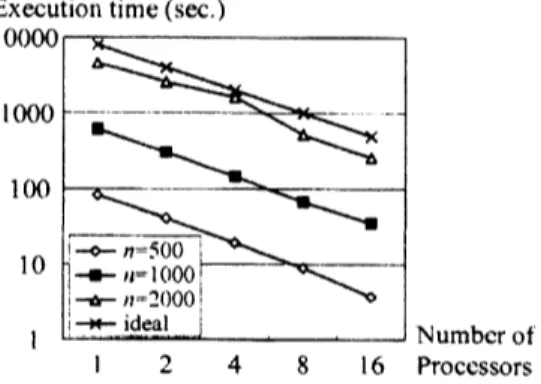
and our algorithm always found the

correct number of eigenvalues in $\Gamma$ with high accuracy. We also show the execution time

as

a function of $n$ and $P$ in Fig. 2. It is clear that almost linear speedup is achieved for

all the

cases.

Figure 1: Computed eigenvalues for the Figure 2: Execution time of

our

algorithm

$n=1000$ and $\epsilon=0.01$

case.

on

Fujitsu HPC2500.

Next we investigated the behavior of

our

algorithm when there are eigenvalues of

multiplicity greater than one. Our test problem is a sma115 $\cross 5$ symmetric quadratic

eigenvalue problem [11] for which $A(z)$ is given by

$A(z)=\{\begin{array}{llll}-z^{2}-3z+1 sym z^{2}-1 -2z^{2}-3z+5 -z^{2}-3z+1 z^{2}-1 -2z^{2}-5z+2 -2z^{2}-6z+2 2z^{2}-2 -4z -9z^{2}-19z+14\end{array}\}$

.

(7)

This quadratic eigenvalue problem has four simple eigenvalues $-4\pm\sqrt{18}$ and $-4\pm\sqrt{19}$

and two eigenvalues 1 and-2 of multiplicity 2.

To solve this problem, we used

as

$\Gamma$ a circle centered at the origin

and with radius

2.1. In this case, two simple eigenvalues and two multiple eigenvalues lie in $\Gamma$

.

In the

eigenvalues, along with the errors and residuals, are shown in Table 2. The multiplicity

of each eigenvalue computed with the method of [1] is also shown in the table. From the

value of the residual, eigenvalues 5 and 6

are

judged to be spurious eigenvalues. So the

number of computed true eigenvalues is four, which coincides with the actual number of

eigenvalues in $\Gamma$

.

In addition, the computed

multiplicity of each eigenvalue was correct.

Thus we know that

our

algorithm

can

be applied to a problem with multiple eigenvalues.

4

Efficient

_{computation of Tr}

$[(A(z))^{-1} \frac{dA(z)}{dz}]$

In ouralgorithm, the computationallydominantpart is the evaluationofTr $[(A(z))^{-1} \frac{dA(z)}{dz}]$

at the $K$ integration points. In the _{implementation used in the previous section, we}

used

LAPACK routines to compute this quantity because the test matrices

were

dense. More

precisely,

we

first computed _{the LU decomposition of} $A(z)$, computed $(A(z))^{-1} \frac{dA(z)}{dz}$ by

repeating forward/backward _substitution $n$ times with $\frac{dA(z)}{dz}$ as the right hand sides, and

then summed up the diagonals ofthe _{resulting matrix to obtain the trace. This process}

requires $O(n^{3})$ work for each integration point.

When the matrixis sparse,

one

can

use

sparse LU decomposition instead to reduce the

computational work. However, the required work is still large. Let Str$(L_{*i})$ and Str$(U_{i*})$

be defined by

Str$(L_{*i})$ $=$ $\{j|j>i, l_{ji}\neq 0\}$ and ₍₈₎

Str$(U_{i*})$ $=$ $\{j|j>i, u_{ij}\neq 0\}$, ₍₉₎

respectively [5]. Then the work to repeat forward/backward substitution $n$ times is

$O(n \sum_{i=1}^{n}\{|Str(L_{*i})|+|Str(U_{i*})|\})$

.

₍₁₀₎

To further reducethe work, a new efficient algorithm for computing Tr $[(A(z))^{-1} \frac{dA(z)}{dz}]$

was

proposed in [14]. Since thisalgorithm

uses

Erisman&Tinney’s algorithmto compute partial elements ofthe inverse of

a

sparse matrix [6],

we

explain the latter algorithm first.

Assume that $A$ is a sparse matrix that admits LU decomposition and its _{$L$ and $U$}

satisfy the following recursion formulae [14]: 1 $c_{ip}$ $=$ $- \sum_{k\in Str(U_{i}.)}u_{ik}c_{kp}\overline{u_{ii}}$’ (11) $c_{pi}$ $=$ $-\underline{1}$

$l_{ii} \sum_{k\in Str(L,:)}c_{pk}l_{ki}$, (12)

$c_{ii}$ $=$ $- \frac{1}{u_{ii}}\sum_{k\in Str(U_{i}.)}u_{ik^{C}ki}+\frac{1}{l_{i1}u_{ii}}$, (13)

where $1\leq i\leq p\leq n$

.

Using these equations, Erisman &Tinney’s algorithm

can

be

described

as

Algorithm 2 below.

[Algorithm2: Erisman&Tinney’s algorithm]

$\{1\rangle$ _{$c_{\eta n}=1/(l_{nn}u_{nn})$}

{2}

do

$i=n-1,1,$

$-1$

$\langle$

3}

Compute

$c_{ip}$ for $p\in$ Str$(L_{*i})$ using eq. (11).

$\langle 4\rangle$ Compute

$c_{pi}$ for $p\in$ Str$(U_{i*})$ using eq. (12).

$\langle$

5}

Compute

$c_{ii}$ using eq. (13).

$\langle$

6}

end do

Afterthe completion of this algorithm, all the elements of$C=A^{-1}$ which are _{situated at}

the nonzero positions of$L^{T}+U^{T}$ are obtained. The computational work ofthis algorithm

is

4$\sum_{i=1}^{n}\{|$Str$(L_{*i})||$Str$(U_{i*})|\}$

.

(14)

Note that this is much smaller than the work of Eq. (10), which would be required if all

the elements of $A^{-1}$

are

computed by repeated forward/backward substitution.

Now

we

show that these partial elements

are

sufficient to compute Tr $[(A(z))^{-1} \frac{dA(z)}{dz}]$.

In the following,

we

denote the elements of $\frac{dA(z)}{dz}$ by $a_{ij}’$

.

First, notice that

Tr $[(A(z))^{-1} \frac{dA(z)}{dz}]=\sum_{i=1}^{n}\sum_{j=1}^{n}c_{ji}a_{ij}’=\sum_{\{i,j|a_{j}\neq 0\}}c_{ij}a_{1j}’$. (15)

Hence only those elements of$C=(A(z))^{-1}$ _{which correspond to the} nonzero _{elements of}

$( \frac{dA(z)}{dz})^{T}$

are

needed. Then

we

use

the following relationship between the

nonzero

positions

of the related matrices:

Nonzero positions of $( \frac{dA(z)}{dz})^{T}$

$\subseteq$ Nonzero positionsof $(A(z))^{T}$

$\subseteq$ Nonzero positionsof $L^{T}+U^{T}$

$=$ Nonzero positions whose value

are

computed by Erisman&Tinney’s

From this relationship, it is clear that the partial elements of$(A(z))^{-1}$ _{obtained by}

Eris-man&Tinney’s

algorithm _{are sufficient to compute ‘Ihr} $[(A(z))^{-1} \frac{dA(z)}{dz}]$

.

Since only

diag-onal elements of $(A(z))^{-1} \frac{dA(z)}{dz}$ need to be computed to evaluate the _trace,

the

computa-tional work required _{in addition to Eq. (14) is} $O( \sum_{i=1}^{n}\{|Str(L_{*i})|+|Str(U_{i*})|\})$, which is

negligible compared with Eq. (14).

We did

some

preliminary experiments _{to evaluate the efficiency of the}

_new

_algorithm

stated above. We used four test matrices shown in Table 3 and compared the execution

times of the two algorithms to compute Tr $[(A(z))^{-1} \frac{dA(z)}{dz}]$ under the condition that the

sparse LU decompositions

are

given. The sparse LU decompositions

were

computed using

the Approximate _{Minimum Degree algorithm [2]. The experiments were performed on a}

Xeon $(2.66GHz)$ _{processor running}

_on

_{Red Hat Enterprise Linux.}

The execution times of the conventionalalgorithmbased

on

repeatedforward/backward

substitution and the new algorithm

are

shown in Table 4. It

can

be

seen

that the

new

al-gorithm is20 to 90 times fasterthan the conventional

one.

Thus

we can

conclude thatthe

new

algorithm is very effectiveinreducing thework reuired tocomputeTr $[(A(z))^{-1\underline{dA(z)}}]$

.

We are now trying to _{incorporate this algorithm into our nonlinear eigenvalue} $so1_{Ver}^{dz}$

5

Conclusion

We proposed

_{a new}

algorithm for the nonlinear eigenvalue problem $A(\lambda)x=0$

.

Our

algorithm _{has the ability to find all eigenvalues within}

_a

_{specified region}

_on

_{the complex} plane. Also, it is expected_{to achieve excellent parallel speedup thanksto the large-grained} parallelism. These advantages have been confirmed by numerical experiments. We also

introduced

a

new algorithm for computing Tr $[(A(z))^{-1} \frac{dA(z)}{dz}]$ efficiently and showed its

effectiveness by preliminary numerical experiments.

More numerical results of

our

algorithm

are

found in [1]. Detailed

error

analysis

Tr $[(A(z))^{-} \frac{(z)}{dz}1$, will be _{given in our forthcoming paper.}

References

[1] T. Amako, Y. Yamamoto, and S.-L. Zhang. A large-grained parallel algorithm for

nonlinear eigenvalue problems and its implementation using OmniRPC. In

Proceed-ings

_of

the 2008 IEEE International

_Conference

on Cluster Computing, pages 42-49,

2008.

[2] P. R. Amestoy, T. A. Davis, and I. S. Duff. An approximate minimum degree ordering

algorithm. SIAM J. Matrix Anal. Appl, 17:886-905, 1996.

[3] J. Asakura, T. Sakurai, H. Tadano, T. Ikegami, and K. Kimura. Anumerical method for nonlinear eigenvalue problems using a contour integral (in Japanese). In

Proceed-ings

_of

the Annual Meeting

_of

JSIAM, pages 133-134, 2008.

[4] T. Betcke and H. Voss. A Jacobi-Davidson-type projection method for nonlinear

eigenvalue problems. Future Generation Comput. Syst., 20:363-372, 2004.

[5] T. A. Davis. Direct Methods

_for

Sparse Linear Systems. SIAM, 2006.

[6] A. M. Erisman and W. F. Tinney. On computing certain elements of the inverse of

a

sparse matrix. Communications

_of

the $ACM,$ $18:177-179$, 1975.

[7] P. Kravanja, T. Sakurai, and M. Van Barel. On locatingclusters of

zeros

ofanalytic

functions. BIT, 39:646-682, 1999.

[8] A. Neumaier. Residual inverse iteration for the nonlinear eigenvalue problem. SIAM

J. Numer. Anal., 22:914-923, 1985.

[9] A. Ruhe. Algorithms for the nonlinear eigenvalue problem. SIAM J. Numer. Anal.,

10:674-689, 1973.

[10] T. Sakurai and H. Sugiura. A projection method forgeneralized eigenvalue problems.

J. Comput. Appl. Math., 159:119-128, 2003.

[11] D. S. Scott and R. C. Ward. Solving symmetric-definite quadratic problems without

factorization. SIAM J. Sci. Stat. Comput., 3:58-67, 1982.

[12] H. Voss. An Arnoldi method for nonlinear eigenvalue problems. BIT Numerical

Mathematics, 44:387-401, 2004.

[13] Y. Yamamoto. A projection method for nonlinear eigenvalue problems based

on

complex contour integration. submitted.

[14] Y. Yamamoto. On computing the diagonals ofthe inverse ofageneral sparse matrix

based

on

the LU decomposition (in Japanese). In Proceedings

_of

the Annual Meeting