A Pincer Randomization Method for Valuing American Options (Mathematical Theory and Applications of Uncertainty Sciences and Decision Making)

(1)

A Pincer

Randomization

Method

for

Valuing

American Options

北海道大学・経済学研究科木村俊一 (Toshikazu Kimura)

北海道大学・経済学研究科鈴木健勝 (Takeyoshi Suzuki)

Graduate School of Economics and Business Administration

Hokkaido University

1 Introduction

Variety has

come

to the options market nowadays since Black

&

Scholes (1973) and Merton (1973)

published the seminal paper. In particular, the valuation of American options (i.e., optionswhich can

be exercised before the pre-specified date)writtenon dividend-payingassetsis animportant issue in the

market due to that they have amuch broader range of applications. Many academics and practitioners

have attempted to resolve the value of American option analytically since McKean (1965) and Merton

(1973) formulated theoptionvalueas afreeboundary problem. However there havebeen

no closed-form

formula and analytical solutions. The difficulties in such pricing options originate from the possibility

ofearlyexercise and the early exercise boundary not known priorimust be determined

as a

part ofthe

solution. Researchers have also made further efforts toward developments of numerical approximation

methods for pricingAmericanoptions.

A brand-new approximation is the randomization method proposed by Carr (1998), which is based

on an American option with a random maturity. The random maturity follows the $n$-stage Erlangian

distribution with mean equal to the pre-specified maturity. Although the idea is easy to understand,

the probability density function (pdf) of Erlangian distribution is not suitable for obtaining a sim ple

formulaforthen-thapproximation. Actually, Carr’sformulafor then-th approximation oftheAm erican

put value is given by

a

recursion of

com

plex triple sums. To improve this shortcoming, an alternative

randomization method hasbeen recently developedby Kimura (2004), which used an order statistic$\mathrm{f}_{\mathrm{o}\mathrm{I}}$

therandom maturity. The order statistic alsoplays akey role in our newrandomization method in this

thesis,andhencethe details ofhismethodwill be specifiedlater. Kimura.i,, approximationnot only hasa

much simpler expressionthanCarr’s one, butalsoits numerical resultshave almost the

same

accuracy as

Carr’s. However,com putationalresults sometimes behave unstablyunderacertain condition. Improving

this inadequacy is a principal goal ofour randomization method, which wecall a pincer randomization.

The primal focus of this thesis ison theAmerican put option because the call

case

canbe analyzed by

put-callsymmetryrelations

The rest of this thesis is organized as follows: In Section 2, we provide

some

prelim inaries for the

analysis. Section 3 provides

an

idea of the pincer randomization method. To examine the accuracy of

our

method, numerical comparisonswith other approximations

are

shown in Section 4. Finally, we give

a conclusion and

some

comments on future researchin Section 5.

2 Preliminalies

2.1 Basic Framework

Assume that the stock price isa risk-neutralized process governedby thestochastic differentialequation

$\frac{dS_{\mathrm{f}}}{s_{t}}=(r-\delta)dt+\sigma dW_{t}$, (2.1)

where $W\equiv\{W_{t} : t\in[0, T]\}$ is a standard Brownian motion process

on

a filtered probability space

$(\Omega, (F_{t})_{t\geq 0},\mathrm{P})$ where $(F_{t})_{t\geq 0}$ is the natural filtration corresponding to $W$ andthe probability

measure

$\mathrm{P}$ is chosen so that the stock has

mean

rate ofreturn$r$. Here, $r$ isthe risk-freerate ofinterest,

$\delta$ is the

dividend rate, and a is thevolatility coefficient of the asset price.

We define the value of American put option with maturity date $T$ and exercise price $K_{\}}$ which

is expressed as $C(S_{t}, t)$ through this article, satisfies the Black and Scholes (1973) partial differential

equation (PDE)

(2)

subject totheboundary conditions

$\lim_{S\downarrow 0}P(S, t)=0$, (2.3)

$\lim_{S\uparrow B_{t}}P(S, t)=K-B_{t}$, (2.4)

$\lim_{S\uparrow B_{t}}\frac{\partial P(S,t)}{\partial S}=-1$, (2.5)

and the terminalcondition

$P(S_{T}, T)=(K-S_{T})^{+}$

.

(2.6)

Equation(2.4)is usually called the “valuematching”conditionandEquation(2.5)isthe “smoothpasting”

condition. These conditions guarantee that premature exercise strategy on the early exercise boundary

$B_{t}$ will beoptimal.

2.2 Randomization Methods

2.2.1 Carr’s randomization

Carr’s randomization method consists of thefollowing three steps:

1. Randomize the maturity $T$ by an exponentially distributed random variable $\tilde{T}$

with mean $\mathrm{E}[\tilde{T}]=$ $\lambda^{-1}=T$in order to value the so-called Canadian option.

2. Extend the result to the

case

that $\tilde{T}$

is distributed as the $n$-stage Erlangian distribution with the

same mean $\mathrm{E}[\tilde{T}]$$=\lambda^{-1}=T$.

3. Takethe limit ofthe randomizedoptionvalue by letting$narrow\infty$toobtaintheunderlyingAmerican

option value

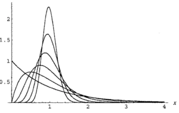
Figure 1 illustrates the $n$-stage Erlangiandistribution converges to Dirac’s delta function concentrated

at the mean $\lambda^{-1}=T$.

$x$

Figure 1: $n$-stage Erlangian probabilitydensity functions$(n =1,2, 4, 8, 16, 32)$

Let$g_{n}^{*}(T)$ $=\mathrm{E}[g(\tilde{T})]$ foracontinuous fimction

$g$. Then,

we

have

$g_{n}^{*}(T)= \int_{0}^{\infty}g(t)\frac{(nt/T)^{n-1}}{(n-1)!}\frac{n}{T}e^{-nt/T}dt$, (2.7)

for whichwe obtain

$\lim_{narrow\infty}g_{n}^{\mathrm{x}}(T)=g(T)$ (2.8)

(3)

2.2.2 Kimura’s randomization

Insteadof the$n$-stage Erlangiandistribution, Kimura(2004)used

an

order static for the randommaturity.

In much the sameway as in Carr’s randomization,his method consists ofthe following three steps:

1. Randomize the maturity $T$ by an exponentially distributed random variable$\overline{T}$

with mean $\mathrm{E}[\tilde{T}]$

$=$

$\lambda^{-1}=T$ in order to valuethe Canadianoption.

2. Extend the result to the case that $\tilde{T}$

is distributed as an order statistic whth the same mean

$\mathrm{E}[\tilde{T}]=\lambda^{-1}=T$

.

3. Take the limit of the randomized option value by letting n,m $arrow\infty$ to obtain the underlying

American optionvalue.

Let $X_{1)}$.

.

’$X_{n+m}$ be independent and exponentially distributed random variables with parameter

$\alpha$

$(>0)$, and let $X_{(i)}$ denote the i-th smallest of these random variables $(\mathrm{i}=1, , . , n+m)$. Thle pdfof

$X_{(7l+1)}$ is givenby

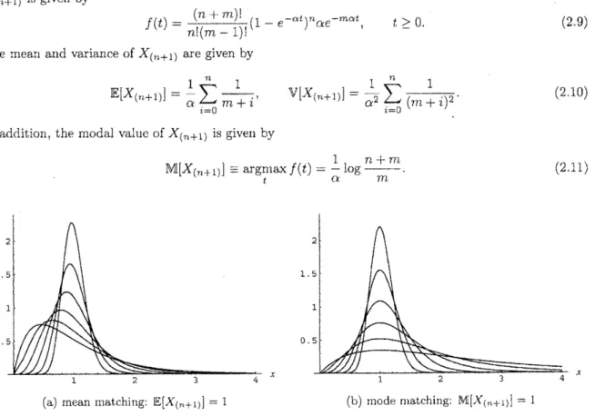
$f(t)= \frac{(n+m)!}{n!(m-1)!}(1-e^{-\alpha t})^{n}\alpha\epsilon^{-m\alpha t}$, $t$$\geq 0$. (2.9)

The mean and variance of$X_{(\uparrow 1+1)}$ are given by

$\mathrm{E}[X_{(\mathrm{n}+1)}]=\frac{1}{\alpha}\sum_{\mathrm{i}=0}^{rx}\frac{1}{m+\mathrm{i}}$, $\mathrm{V}[X_{\langle n+1)}]=\frac{1}{\alpha^{2}}\sum_{i=0}^{n}\frac{1}{(rn+\iota)^{2}}$. (210)

In add ition, the modal value of$X_{(7b+1)}$ is given by

NI$[X(7\downarrow+1)]\equiv \mathrm{a}\mathrm{r}\mathrm{g}\mathrm{n}t$lax$f(t)= \frac{1}{cx}\log\frac{n+m}{m}$. (2.11)

1

0

$X$ $X$

(a) mean rnatching $\mathrm{E}[X_{\{n+1)}]=1$ (b) mode$\Pi 1\mathrm{a}\mathrm{t}\mathrm{c}\mathrm{h}\mathrm{i}_{\mathrm{I}\mathrm{l}}\mathrm{g}$. $\mathrm{M}|X(n+1)]=1$

Figure 2: Probability densityfunctions ofthe order statistic $(n=m=1, 2,4, 8, 16, 32)$

Figure $2(\mathrm{a})$ and $2(\mathrm{b})$ show theconvergence of the pdfas $n(=m)arrow\infty$

.

There is not all that much

difference between these figures and they converge to Dime’s delta function concentrated at the mean

$\mathrm{E}[X_{(7\iota+1\}}]=1$. By setting either $\mathrm{E}[X_{(n+1)}]=T$or$\mathrm{N}\#[X_{(\tau\iota+1)}|--T,$ $X_{(n+1)}$ canbe another candidate for

the random maturity$\tilde{T}$

, because $1\mathrm{i}\ln_{\mathit{7}1,marrow\infty}\mathrm{V}[X(n+1)]-\wedge 0$

.

Kimura (2004) adopted the mode-m atching NI[X(n+l)]=T in his randomization for $\mathrm{c}\mathrm{o}$ mputational

convenience,because thereisnosignificantdifferencebetweenthe twomatchings. For the mode-matching,

a can be determined by

$\alpha=\frac{1}{T}$ltog$\frac{n+m}{m}$. (2.12)

For acontinuous function $g(t)(t\geq 07$,let $g_{\iota}^{*},,n\iota$ $\equiv g_{l,7n}^{*},(T)$

$=\mathrm{E}[g(\tilde{T})]$, $\mathrm{t}\}_{1}\mathrm{e}\mathrm{n}$

(4)

forwhich we have

iim $g_{n,m}^{*}(T)=g(T)$

.

(2.14)

$n,r’\iotaarrow\infty$

Proposition 1 (Kimura) The sequence

$(g_{r\iota,m}^{*})_{r\iota,\tau n\geq 1}$ satisfiesthe recursion

$\{$

$g_{0,m}^{*}=I_{0}^{\infty}$rnae$-mc\iota tg(t)dt$

$g_{n,m}^{*}= \frac{n+m}{n}g_{n-1,m}^{*}-\frac{m}{n}g_{n-1,m+1}^{*}$, $n\geq 1$

.

(2.15)

Let $L^{*}(m\alpha)$ denote arootof the equation for the eaxly exercise boundary of Canadian options. The

$7\mathrm{V}$-th randomized approximation $g_{N,N}^{*}\equiv\beta_{N}\approx B_{t}(N\geq 1)$ can be obtained by the algorithm named

OS-Random.

The algorithm also

can

be applied to computing the option value $F(t, S)$ by assuming that we have

a functional programforcomputing$P^{*}(m\alpha, S)$ for a setofthe parameters $\{t, S, K,T, r, \delta, \sigma\}$

.

2.3 Canadian Options

Therandomization methods are based on the valueofCanadian option whosematurity is exponentially

distributed to introduce not only Carr’s randomization but aiso the alternativeoneproposed byKimura

(2004).

Proposition 2 (Kimura) The value of the European-style Canadian put optionis given by

$p^{*}(\lambda, S)=\{$ $\xi(S)+\frac{\lambda}{\lambda+r}K-\frac{\lambda}{\lambda+\delta}S$, $S<K$ $\eta(S)$, $S\geq K$, (2.16) where $\xi(S)=\frac{1}{\theta_{+}-\theta_{-}}\frac{\lambda}{\lambda+\delta}(1-\frac{r-\delta}{\lambda+r}\theta_{-})K(\frac{S}{K})^{\theta_{+}}$ , $S<K$ $\eta(S)=\frac{1}{\theta_{+}-\theta_{-}}\frac{\lambda}{\lambda+\delta}(1-\frac{r-\delta}{\lambda+r}\theta_{+})K(\frac{S}{K})^{\theta_{-}}$, $S\geq K$, (2.17)

and the parameters $\theta\pm$

are

tworoots of the follow ing quadraticequation

$\frac{1}{2}\sigma^{2}\theta^{2}+$$(r- \delta -\frac{1}{?}.\sigma^{2})\theta-(\lambda+r)=0$, (2.18)

$\mathrm{i}.e.$,

$\theta_{\pm}=\frac{1}{\sigma^{\underline{9}}}\{-(r-\delta-\frac{1}{2}\sigma^{2})\pm\sqrt{\langle r-\delta-\frac{1}{2}\sigma^{2})^{2}+2\sigma^{2}(\lambda+r)}\}$

.

(2.19)

Proposition 3 (Kimura) For $L^{*}\leq K$, the value of the American-style Canadian put option is given

by $P^{*}(\lambda, S)=\{$ $K-\mathit{3}$, $S\leq L^{*}$ (2.20) $p^{*}(\lambda, S)+e^{*}(\lambda, S)$, $S>L^{*}$, where

(5)

3 A

Pincer

Randomization Method

Kimura’s randomization method is notonly much simpler than Carr’s one, but also as accurate as Carr’s

one; however themethodshows unstable behaviors near the expiryundercertain conditions. Thereasons

for the unstabilityareconsidered as

(i) the algorithmis sensitive to theprecision of the root $L^{*}$.

(ii) the$(n, m)$-thapproximation$g_{n,m}^{*}$ cannot appropriately satisfies the value matching conditionin the

recursiveprocedure.

In this section, we propose a new randomization scheme named a pincer randomization (PR) method

to

overcome

those difficulties. The PR method is based on a pair of lower and upper bounds for a

true value (say TRUE), and then TRUE is sandwiched in between the bounds. This methods reflect

some fundamental properties ofthe option Greek Theta and the order statistic. It is generally known

that Theta indicates the ratioof thechange in an American putoptionprice to the decrease in time to

expiration, so that the shorter theremaining time to expiration, theoption value ischeaper.

Remark 1 Note that the relation of apair oflower and upper bounds inverts if and only if the Theta

is negativeunder deep-in-the-money.

3.1 Lower and upper bounds

for

the option

value

Assume that thematurity $T$ is arandom variable $\tilde{T}$

distributed

as

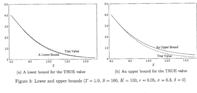
the order statistic$X(n+1)$ with mean

$\mathrm{E}[\tilde{T}]=T$, as in the OS-Random algorithm. From Figure $2(\mathrm{a})$ andthe Theta property of Americanput

options that the

mean-m

atchingapproximation for the option value always underestimates the truevalue

when $n$,$m$ is not large enough, giving a lower bound. Note that mean-matching approximation for the

earlyexerciseboundary providesthe upper bound. Figure $3(\mathrm{a})$ shows that the lower bound $\mathrm{i}_{\mathrm{b}}$ atight one

over

the true value derivedby theCRR binom ialmethod with $n=$ 1000.

In the

same manner

as the mean-matching case, Figure $2(\mathrm{b})$ and theTheta property shows that the

mode-matching approximation always overestimates the true valuewhen$n$,$m$is small, $\mathrm{i}.e.$, it isanupper

bound For the early exercise boundary, the mode-matching approximation providesthe lower bound

Figure $3(\mathrm{b})$ shows that the upper bound is less tight than the lowerbound, whereTRUE values

are

also

computed by the CRR binomial methodwith$n$ $=$ 1000.

50

(a) A lower bound for theTRUEvalue (b) An upperbound for theTRUEvalue

Figure 3: Lowerand upperbounds $(T=1.0, S=100, K=100, r=0.05, \sigma=0.3, \delta=0)$

3.2 Interpolating

lower and

upper

bounds

Figure 4illustrates arelationship betweenthe lower and upperbounds for the early exercise boundary.

This figure shows that thetheTRUEvalue is appropriatelysandwichedinbetween thebounds, and that

(6)

Figure 4: Lower and upper bounds for theearly exercise boundary ($K=100$,$r=0.05$, a $=0.3$, $\delta=0$)

option value, the TRUE value is appropriately sandwiched in between the bounds, and the lower bound

is agood approximation for theTRUE

one.

From Figure 3, the

mean

matching provides

more

accurate

approxim ations for the option value. Prom these observations, we employ the two methods below for

valuingAmerican put options.

.

Arithmetic Average:

$P_{A}\langle t$,$S_{t}$) $= \frac{L(t,S_{t})+U(t,S_{t})}{2}$ (3.1)

where $L(t, S_{t})$ and $U(t, S_{t})$ are the lower and upper bound for the option va$\mathrm{l}\mathrm{u}\mathrm{e}$, respectively.

.

Geometric Average:

$I_{G}^{\supset}(t, S_{\mathrm{t}})=\sqrt{L(t,S_{t})\mathrm{x}U(t,S_{t})}$ (3.2)

As described above, the upper bound of the earlyexercise boundary and the lower bound of the option

value

are

good approximationsfor theTRUEvalues. Hence,wealso add the lower-boundapproximation

for theoption value in comparisons.

0 0

0 -0

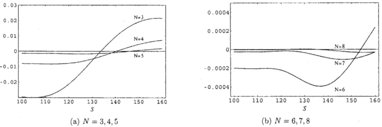
(a) $N=3$, 4,$!\mathrm{J}\ulcorner$ (b) $N=6$,7, 8

Figure 5: Relative percentage

errors

of the approxim ations for the vanilla European put value $p(0, S)$

$\langle$$T=1.\mathrm{O}$, $K=1\mathrm{O}\mathrm{O}$, $r=0.05$, a $=0.3$, $\delta=0.05$)

To determine the level 1V of the approximation,

we

make a comparison between $p(t, S)$ and its PR

approxim ation. Obviously, the exact values of $p(t, S)$

can

_{be computed by} the Black-Scholes formula

$(2,2)$, Figure 5 illustrates the relative percentage

errors

of approximations for$p(0, S)$

as

functions of$S$.

The approximations become better as $N$ increases and wehavesufficient accuracy for$N\geq 6$

.

Hence, we

(7)

4 Computational

Results

Figure $6(\mathrm{a})(6(\mathrm{b}))$ shows

some

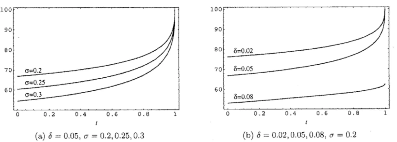
relations between theearlyexerciseboundaryand the volatiliry (dividend

rate). Also, Figure $7(\mathrm{a})(7(\mathrm{b}))$ shows

som

ne relations between the option values and the volatility

(ma-turity). In order to check the performance of the PR method in detail, we

com

npare them with other

approximations for particular

cases

quoted from numerical experiments in AitSahlia and Carr (1997).

Tables 1 and 2 summarize these results, in which we compute three approximation by the PR method

withboththe arithmeticandgeometricaverages and the lower-bound approximationnam ed LB-Rondorn.

We employ the arithmetic average of the 1000- and lOOl-steps binomial value

as

a bench mark of the

TRUE value. For the methods of OS-Random, Carr, and Geske

&

Johnson, ‘.N-pts” in these tables

denote the numberofstepsofthe$N$-point Richardsonextrapolation. For the finite-difference results, the

parameters $N$ and $M$ denote the numbersof time and state steps, respectively. SeeAitSahlia and Carr

(1997) for details oftheir experiments.

$t$

(a) $\delta=0.05$, $\sigma=0.2$_,0.05,0.3 (b) $\delta=0$02,$00_{\iota}^{r_{\mathrm{J}}}$, 0.05, $\sigma$ $=02$

Figure 6: Earlyexercise boundaries ofput options $(K=1\mathrm{O}\mathrm{O}, T=1.\mathrm{O}, r=0.05)$

(a) T$=1.()$_, _a $=0$2,0.3,$().4$ (b) T$=0.05$,10, 1.0,$\sigma=02$

Figure 7: Valuesofput options $(K=1\mathrm{O}\mathrm{O}, t=0, r=0.05, \delta=0.02)$

The PR methodperforms very well and competes with OS-Random and Carr’s randomization, In

addition,the PRmethod succeeds in the waythatmodificationofOS-Randomthatalwaysunderestimates

the TRUE value, because the PR method provides not only much

more

accurate approximations for

valuing put options but also better approximation than OS-Randomn In addition,

we see

from these

figures that thePR method is

more

accurate than LBA and LUBA, which are also thelower-bound and

the lower-and-upper-bounds approximations, respectively.

Table 1 shows the impacts of the initial stock price $S$. The PR method $\mathrm{w}\mathrm{i}\mathrm{t}\mathrm{h}_{1}$ both of arithmetic

and geometric average becomes accurate as $S$ increases, because the early exercise prem iu1n relatively

(8)

that thePR method canvalue European option valuesas accurate astheBlack-Scholes formula and that

wecan decomposeAmerican option value into the early exercise premium plus Europeanoption value.

Table 2 demonstrates that remaining time impacts on the option values. The PR method with

both arithmetic and geometricaverages becomesaccurate as the remaining time becomes long. Forthis

tendency, we

can

give thesameprospect fromTable 1. Inaddition, fromTables 1and2,

we

can see that

the PR method with arithmetic average is accurate enough and is greater than theonewith geometric

average. Clearly, this reflects the fact that $P_{A}(t, S_{t})\geq P_{G}(t, S_{t})$for all $(t, St)$.

From the observations in Figures 3 and 4, it

was

considered that the lower-bound approximations

for the option values would perform well. However, we see from Tables 1 and 2 that the lower-bound

approxim ations are less accurate than other approximations. We alsosee from othernumerical

experi-ments that the randomization method with

mean

matchingperforms well ifandonlyifdividendis zero

forwhich the root $L^{*}$ canbecompiited via

$L^{*}=K( \frac{r(\theta_{+}-1)}{\lambda})\frac{1}{\mathit{0}_{+}}$ (4.1)

without using Newton’s method. These observations wouldimply that the accuracy of the lower-bound

(or mean-matching) approximation is highlysensitive to thecomputational accuracy oftheroot $L^{*}$

.

5 Conclusion

The previous randomization methods have crucial problems such

as

(i) difficulty of implementation for

Carr’s one and (ii) unstable behavior

near

expiry for Kimura’s

one.

To rectify these faults at the same

time,wehaveemployed an interpolationapproximationusing apair oflowerandtipperboundsobtained

byKimura’s randomization method. The ideais based onthe Theta property of American put options.

Our new method, thePR method,refines Kimura’sone, removing another fault ofunderestimation.

The PR method generates accurate approximations when theinitial stockprice is intheout-of-money

or the remaining time to maturity is long. It is straightforward to interpret these properties frorn the

fact that American option value can decomposed into the early exercise premium and the associated

Europeanoption value,the latter of which constitutes agreater portion of the wholevalue. However , the

PRmethod still haveatendency of underestimation from the true value, whichneeds a further revision

of the randomization.

Mathematically,theessentialof randomization canbe interpretedas

an

inversionofLaplace

or

Fourier

transforms.

Thisinterpretationenables

us

to apPly the random izationmethodsincluding the PRmethod

to valuing other options, $e.g.$, exoticor path-dependent options such asAsian, lookback, barrier options

and

so on.

This isafuture theme of extensive research. Another extensionof the randomizationmethod

is the

case

that the stock return jumps accidentally, that is, the stock price process follows not the

Brownian motion butajum $\mathrm{p}$-diffusionprocess suchas Levyprocesses. This remainsasfuturework, too.

References

[1] AitSahlia, $\mathrm{F}_{\}}$.and Carr, P., 1997, “American Options: A Comparison of Numerical

$\mathrm{M}\mathrm{e}\mathrm{t}\mathrm{h}\mathrm{o}\mathrm{d}_{\mathrm{S}},$

)’

Nu-merical MethodsinFinance,L C.G. RogersandD. Talay (eds.), CambridgeUniversity Press, 67-87.

$\lfloor\lceil 2]$ Black, F., and M. Scholes, 1973, “The Pricing of Options and Corporate Liabilities,” Journal

of

Political Economy, 81, 637-659.

[3] Carr, P., 1997) “Randomization and the American Put,” Review

_of

FinancialStudies, 11, 597-626.

[4] Cox, J.C.,

_S.A.

_Ross_and _M. Rubinstein, 1979, “option Pricing; ASimplified Approach,” Joumal

_of

Financial Economics, 7 229-264,

[5] Kimura, T., 2004, “Alternative Randomization for Valuing American Options,” The 2004 Daiwa

InternationalWorkshop on Financial Engineering, Kyoto, Japan.

[6] McKean, H.P., Jr., 1965, “Appendix: A Free Boundary Problem for the Heating Function Arising

from aProblem in Mathematical Economics,” IndustrialManagement Review, 6,

32-39.

[7] Merton, R., 1973, “Theoryof Rational OptionPricing,” Bell Journal

_of

Economics andManagement

(9)

$\mathrm{T}\mathrm{a}\cdot\frac{\mathrm{b}1\mathrm{e}1.\mathrm{A}\mathrm{c}\mathrm{o}\mathrm{m}\mathrm{a}\mathrm{r}\mathrm{i}\mathrm{s}\mathrm{o}\mathrm{n}}{\mathrm{M}\mathrm{e}\mathrm{t}\mathrm{h}\mathrm{o}\mathrm{d}}$of approximationsfor$P(0,S)S=\mathrm{S}0(T=3,K=100,r=0.06, \sigma=0.4,\delta=0.02)S=90S=100S=110S=120$

Binomial 29.2601 24.8023 21.1294 18.0849 15.5428

PRmethod (Arithmetic Ave.) 28,8392 24.4533 20,8489 17.8681 15.3892

PR method (Geometric Ave.) 28.8373 24.4501 20.8445 17.8624 15.3823

LB-Random 28.5135 24.0614 20.4092 17.3971 14.9005

OS-Random (8-Pts) 28.7998 24.4246 20.7891 17.7971 15.2995

Carr (3-pts)

29.2323

24.7692 21.0835 18.0369 15.4873

Geske and Johnson

31.0305

26.1543 22.1114 18.7646 15.9911

Quadratic

29.4377

25.0614

21.4484 18.4418 15,9239

LBA 29.2105 24.7669 21.1039 18.0635 15.5252

LUB A 29.2540 24.7989 21.1306 18.0860 15.5437

Bunch and Johnson

29.938225.1566

21.3092 18.1558 15.5755

Huang et al. 29.7147 25.0136 21.2121 18.1173 15.5729

$\underline{\mathrm{F}\mathrm{i}\mathrm{n}\mathrm{i}\mathrm{t}\mathrm{e}\mathrm{D}\mathrm{i}\mathrm{f}\mathrm{f}\mathrm{e}\mathrm{l}\mathrm{e}\mathrm{n}\mathrm{c}\mathrm{e}(N=200,\lambda f=300)}$

29.058424.4744

20.633014.5535

14.5535

$\frac{\mathrm{T}\mathrm{a}\mathrm{b}1\mathrm{e}2\cdot \mathrm{A}\mathrm{c}\mathrm{o}\mathrm{m}\mathrm{p}\mathrm{a}\mathrm{r}\mathrm{i}\mathrm{s}\mathrm{o}\mathrm{n}\mathrm{o}\mathrm{f}\mathrm{a}\mathrm{p}\mathrm{p}\mathrm{r}\mathrm{o}\mathrm{x}\mathrm{i}\mathrm{m}\mathrm{a}\mathrm{t}\mathrm{i}\mathrm{o}\mathrm{n}\mathrm{s}\mathrm{f}\mathrm{o}\mathrm{r}P(0,100)(K.=100,r=0.06,\sigma=0.4,\delta=0.02)}{\mathrm{M}\mathrm{e}\mathrm{t}\mathrm{h}\mathrm{o}\mathrm{d}T=0.5T=10T=1.5T=2.0T=2.5}$

Binomial

$\overline{10.2741}$

13.877416.3682

18.284019.8349

PR method (Arithmetic Ave.)

10.3057

13.8392

16.2596

18.1109

19.6045

PR method (Geom etric Ave.)

10.3016

13.8345

16.2547 $[perp] 8\prec.1061$ 19.5998

LB-Random

10.0157

13.4765 15.8586

17.6884

19.1702

OS-Random (8-pts) 10.1802 13.7083 16.1399 18.0090 19.5321

Carr (3-pts) 10.2759 13.8670

16.3469

18.2533 19.7960

Geske and Johnson 10.3159 14.0553 16.7200 18.8388 20.5970

Quadratic 10.2728 13.9142

16.4627

18.4476 20.0743

LBA 10.2697 13.8G79 16.3545

18.4476

19.8134

LUBA 10.2750 13.8796 16.3712 18.2869 19.8371

Bunch and Johnson 10.2679 13.8904 16.4070 18.3487

19.9434

Huang et al. 10.2813

13.8756

16.3657