Quantitative Operational Risk Management : Properties of Operational Value at Risk (OpVaR) (Financial Modeling and Analysis)

Quantitative Operational Risk Management:

Properties of Operational Value at Risk (OpVaR)

Takashi Kato

Division ofMathematical Science for Social Systems, Graduate School of Engineering Science

Osaka University

1

Introduction

BaselII (International Convergence of CapitalMeasurement and Capital Standards: A Revised Framework)

was

published in 2004, andin it, operational risk

was

added

as a new

risk category.

The Basel Committee on Banking Supervision [2] defines operational risk

as

“the risk of loss

resulting from inadequate or failed internal processes, people and systems or from extemal events. This definition includeslegalrisk, but excludes strategic andreputational risk” (seealso McNeil et al. [19]$)$

.

For measuring the capital charge for operational risk, banks may choose from three

ap-proaches: thebasicindicatorapproach(BIA), the standardizedapproach ($SA$),and theadvanced

measurement approach (AMA). While BIA and $SA$ provide explicit formulas, AMA does not

specify

a

model for quantifying risk amount (risk capital). Hence, banks adopting AMA must construct their own quantitative risk models and conduct periodic verification.

Basel II states that “a bank mustbe able to demonstrate that its approach captures

poten-tially

severe

‘tail’ loss events”, as well as that “a bank must demonstrate that its operational

risk

measure

meets a soundness standardcomparableto aone year holdingperiod and a 99.$9th$

percentile _{confidence interval” [2]. The value-at-risk} $(VaR)$ with a confidence level of0.999 _is a

typical risk measure, and therefore

we

adopt such operational $VaR$ (abbreviated

as

OpVa$R$).

In this paper, we focus the following two topics:

(i) Analytical methods for calculating OpVa$R$

(ii) _{Asymptotic behavior of OpVa}$R$

Item (i) is important fromapracticalratherthan theoretical viewpoint. Infact, many banks adopt the so-called loss distributional approach (LDA) and calculate OpVa$R$ by using Monte

Carlo ($MC$) simulations. _However, $MC$ simulations are not optimal in _{terms of computation}

speed androbustness. We pointout the problems associated with $MC$ and introducealternative

analytical methods forcalculating OpVa$R$ in the LDA model.

Item (ii) is a theoretical issue. It is well known that distributionsofoperationalrisk amount are characterized by fat tails. In this study, we show the asymptotic behavior of the difference

between the$VaRsVaR_{\alpha}(L+S)$and$VaR_{\alpha}(L)$ ($\alpha$denotes the confidence level of$VaR$) for

heavy-tailed random variables$L$and$S$with$\alphaarrow 1$($=$

100%)

as

anapplicationto the sensitivity analysis

of quantitative operational risk management in the framework of AMA. Here, the variable $L$

denotes the loss amount of the current risk profile, and$S$indicatesthe loss amount caused by

an

the thicknesses of the tails

of

and

.

In particular, if the tail of is sufficiently thinner

than that of $L$, then the difference betweenprior and posterior risk amounts is asymptotically

equivalent to the expected lossof $S$, i.e., $VaR_{\alpha}(L+S)-VaR_{\alpha}(L)\sim E[S],$ $\alphaarrow 1.$

2

Analytical

methods

for

calculating

OpVa

$R$

2.1

LDA Model

As mentioned above, banks who adopt AMA can use an arbitrary model to estimate OpVa$R.$

In actuality, however, most banks choose the LDA, in this section, we briefly introduce the

definition of LDA.

Let $L$ be

a

random variable that denotes the total loss amount in

one

year. In the LDA

framework, the distribution of$L$is

constructed on

the basis of the following two distributions:

.

Loss severity distribution $\mu\in \mathcal{P}([0, \infty))$,

.

Loss frequencydistribution $\nu\in \mathcal{P}(\mathbb{Z}_{+})$

.

Here,

we use

$\mathcal{P}(D)$ to denote the set of all probability distributions defined on the space $D,$

where $z_{+}=\{0,1,2, \ldots\}$

.

Let $N$ be

a

random variable distributedby$\nu$ and $(L_{k})_{k}$ be

a

sequence

of identicallydistributedrandomvariablesdistributed by $\mu$

.

We regard$N$

as

the number of loss events in a year and $L_{k}$

as

the amount ofthe kth loss. Then, the total loss amount $L$ is given

by

$L= \sum_{k=1}^{N}L_{k}=L_{1}+\cdots+L_{N}$

.

(2.1)

We

assume

that all randomvariables $N,$$L_{1},$ $L_{2},$

$\ldots$

are

independent.

This model is closely related to theso-called Cramer-Lundberg model, whichis widely used

inactuarialscience. Wenote that $L$becomesthe compound Poissonmodelwhen$\nu$is the Poisson

distribution. Inoperational risk management, the LDA model is applied to each event type

or

business line. For instance, ifa bank has $M$ event types, then the total loss amount $L^{i}$ ofthe ith event type is given by (2.1) with a severity distribution $\mu_{k}$ and a frequency distribution

$\nu_{k}$. Then, the “bank-wide” total loss amount is given by the sumof $L^{1},$

$\ldots,$

$L^{M}$

.

However, for

simplicity, we ignore the characteristics of different event types and business lines in this paper

since

our

purpose is to calculate the $VaR$and OpVa$R$

$VaR_{\alpha}(L)=\inf\{x\in \mathbb{R} ; P(L\leq x)\geq\alpha\}$ (2.2)

of$L$as defined in (2.1) witha confidence level $\alpha=0.999.$

A characteristic property of distributions of operational losses is a fat tail. It is well known that operational loss distributions are strongly affected by loss events with low frequency and

substantial loss amount. Thus, we should set $\mu$ as a heavy-tailed distribution to capture such

generalized Pareto distribution (GPD):

LND$(\gamma, \sigma)((-\infty, x])$ $=$ $\int_{0}^{x}\frac{1}{\sqrt{2\pi}\sigma y}\exp(-\frac{(\log y-\gamma)^{2}}{2\sigma^{2}})dy(x\geq 0)$, $0(x<0)$,

GPD$(\xi, \beta)((-\infty, x])$ $=$ $1-(1+ \frac{\xi}{\beta}x)^{-1/\xi}(x\geq 0)$, $0(x<0)$

.

Here, $\gamma,$$\beta>0$

are

location parameters and $\sigma,$$\xi>0$ are shape parameters. Larger values of$\sigma$

and $\xi$ yield

a

fatter tail of the severity distribution. In fact, GPD

is a representative fat-tailed

distribution andplays

an

essential rolein extreme value theory (EVT). For details

on

EVT,

see

[11].

2.2

$MC$

Simulation

The most widely used method for calculating (2.2) is $MC$ simulation. The _{algorithm for}

calcu-lating OpVa$R$by $MC$ simulation isas follows:

1. Generate$a$ (pseudo)random variable $N$ distributed by $\nu.$

2. Generate i.i.$d$

.

(pseudo)random variables _{$L_{1},$}

$\ldots,$$L_{N}$ distributed by$\mu.$

3. Put $L=L_{1}+\cdots+L_{N}.$

4. Repeat steps $1-3m$ _{times (}$m$ is the number of simulation iterations). Then, we obtain$m$

independent copies of$L.$

5. Sort the variables $L^{1},$

$\ldots,$$L^{m}$ such that $L^{(1)}\leq\cdots\leq L^{(m)}.$

6. Set $VaR_{\alpha}^{MC}(L)=L^{([m\alpha])}$, where $[x]$ is the largest integer not greater than_$x.$

The estimator$VaR_{\alpha}^{MC}(L)$ isanorder statistic of_{$VaR_{\alpha}(L)$}. Letting

$marrow\infty,$ $VaR_{\alpha}^{MC}(L)$converges

to $VaR_{\alpha}(L)$ under

some

technical conditions.

$MC$ is an extremely useful method which is widely _{adopted in practice because of its}

_ease

of implementationand _{wide applicability. However, it is known to suffer from several problems,}

one

ofwhich is that it requires

a

large number of simulation iterations (i.e., $m$ should be very

large). The

reason

is that convergenceof$VaR_{\alpha}^{MC}(L)$ is generally veryslow. Another problem is

that the estimated value $VaR_{\alpha}^{MC}(L)$ is unstable for some specific distributions. In the following

subsections, weexamine theseproblems numerically.

2.2.1 Test 1: Simulation Iterations and Computation Time

Until the end ofSection2, weadopt the Poissondistributionwithanintensity$\lambda$

as

the frequency

distribution $\nu$ :

$\nu(\{k\})=$Poi$( \lambda)(\{k\})=\frac{\lambda^{k}e^{-\lambda}}{k!},$

$k\in z_{+}.$

We investigate the number of simulation iterations $m$ required for estimating OpVa$R$ with a

by using the Pritsker method with a 95% confidence level. We iterate the above $MC$ algorithm

while increasing $m$ until

$\frac{VaR_{\alpha}^{MC,upper}(L)-VaR_{\alpha}^{MC,1ower}(L)}{VaR_{\alpha}^{MC}(L)}<0.01,$

is satisfied, where$VaR_{\alpha}^{M}C$,upper_$(L)$ and $VaR_{\alpha}^{MC,1ower}(L)$ areorder statistics satisfying

$P(VaR_{\alpha}^{MC}$ ’lower$(L)\leq VaR_{\alpha}(L)<VaR_{\alpha}^{MC}$’upper$(L))\simeq 0.95.$

For

an

explanation of how to obtain the values of$VaR_{\alpha}^{M}C$,upper_$(L)$ and $VaR_{\alpha}^{MC,1ower}(L)$, please

refer to [26]. Note again that the estimated value of $m$ obtained by the above procedure is

not exact. Nevertheless, it is obvious that

a

substantial number of simulation iterations

are

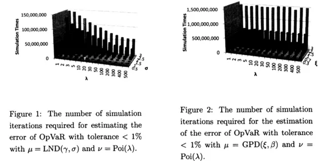
necessaryto obtain the estimator of OpVa$R$withtolerable accuracy. Figure 1 givesthenumber

of simulationiterations in the

case

of$\mu=$LND$(\gamma, \sigma)$. We

see

that manyiterations

are

necessary

when $\sigma$is large and

$\lambda$ issmall. Figure2corresponds to the

case

of

$\mu=$ GPD$(\xi, \beta)$

.

This implies

that the number of iterations is similarly large when $\xi$ is large, but in contrast to the

case

of

LND, the number of iterations is unaffected bythe value of$\lambda$. This difference is caused by the

tail probability function of LND is rapidly varying while that ofGPD areregularly varying (see [4] and [11] for details). Here, weremark that the location parameters $\gamma$ and $\beta$ do not influence

the number ofsimulation iterations.

These results indicate that the$MC$ methodrequires

a

huge number of simulationiterations,

especially when the values ofthe shape parameters $\sigma$ and $\xi$

are

large, that is, when $\mu$ is fat-tailed. In this case, long computation time is required: ifwe conduct

a

calculation with $\xi=3$

and $\lambda=500$,

as

in Figure 2, the computation would require

more

than2 days to complete

on a

typical personal computer.

$1,500,000,000$

150,000,000 $v\infty$

$\in v\infty$ $\vdash 1,000,000,000\underline{\in}$

$\underline{\underline{F\circ e}\check{\varpi}}100,0\infty,0\infty$ $\frac{\underline{\circ\epsilon}\dot{\varpi}}{3,\frac{\in}{\dot{\mathfrak{n}}}}$ 500,000,000 $\in 3$ 50,000,000 $\dot{\overline{\omega}}$ $0$ $0$ $\zeta$

Figure 2: The number of simulation

Figure 1: The number of simulation

iterations required for the estimation

iterations required for estimating the

error of OpVa$R$ with tolerance $<1\%$ of the error of OpVa

$R$ with tolerance

with $\mu=$LND$(\gamma, \sigma)$ and $\nu=$Poi$(\lambda)$

.

$<$ 1% with _$\mu=$ GPD$(\xi, \beta)$ and _$\nu=$

Poi$(\lambda)$

.

such

as

multithread programming and general-purpose computing

on

graphics processing units (GPGPU), this entails high development cost.

2.2.2 Test 2: Accuracy for Specific Distributions In this test, we calculate $VaR_{\alpha}^{MC}(L)$ in the case where

$\mu$ is derived empirically. We generate

500 sets of dummy loss data (“virtual” realized data) and 15 sets of scenario data based

on

GPD(1.2, 100, 000). Then,

we

set $\mu$

as

the empirical distribution definedby these data. Figure

3shows the tail probability functionof the severitydistribution

on a

log-log scale. We also take $v=Poisson(500)$

.

We conduct 100 calculations of $VaR_{0.999}^{MC}(L)$ (with 1,000,000 iterations) as OpVaR. Figure

4 shows

a

histogram of

100

estimations of OpVaR. Clearly, the distribution of OpVaRs is

bi-polarized. This

can

be explained by using Theorem 3.12 in [5]: $VaR_{O.999}(L)$ is approximated

by $\hat{v}\equiv VaR_{0.9998}(L_{1})$. Here, $\hat{v}$ is the 99.$9998th$ percentile point of

$\mu$. In fact, the empirical

distribution $\mu$ has a large point

mass

at the 99.$99988th$ percentile point. This is near $\hat{v}$, and

thus the value of the simulated OpVa$R$is sensitive to the above loss data.

This indicates that the $MC$ method may result in serious _estimation

error

_{in calculating}

OpVaR. Note that the severity distribution used in this numerical experiment is not far from

a

standarddistribution, and such a phenomenon is conceivable in practice.

$1.E+00 1.E+03 1.E+06 1.E+09 1.E+12 1.E+15$ $\sim 0.\approx\dot{\sim}\sim\dot{\sim}\infty\tilde{\dot{\infty}}\check{\dot{n}}\vee\Phi\infty 0\circ\dot{\circ}\vee\cdot\vee\vee\vee\cdot\vee\dot{\emptyset}\infty 0\sim\vee\infty\infty oX\check{\infty}$

$x$

$v\circ|ues$of OpVoR($/10\wedge 11)$

2

:

realized loss data

$\bullet$

:

scenariodata

Figure 4: Histogram of 100 estima-tions of OpVa$R.$

Figure 3: Log-log graph of the tail probability function $\mu((x, \infty))=$

$P(L_{1}>x)$

.

2.3

Analytical Computation Methods

In Section 2.2,

we

point out

some

of the problems associated with the $MC$ method. In this

section,

we

introduce

some

alternative methods for calculating OpVa$R.$

There have been studies on probabilistic approximations for the LDA $mo$del. In particular, a closed-form approximation (Theorem 3.12 in [5]) is well-known and widely used for rough

calculation ofOpVa$R$:

$VaR_{\alpha}^{EVT}(L)=VaR_{1-(1-\alpha)/\lambda}(L_{1})$

.

If $\mu$ is subexponential, then

$VaR_{\alpha}^{EVT}(L)$ converges to $VaR_{\alpha}(L)$ as $\alphaarrow 1$

.

Thus, $VaR_{\alpha}^{EVT}(L)$

approximates $VaR_{\alpha}(L)$ when $\alpha$ is close to 1. Usually,

we

can calculate

$VaR_{\alpha}^{EVT}(L)$ almost

instantly because we assign the explicit form of $\mu$ in most

cases.

This approximation method

alsoplays

an

importantrole inEVT,and in

Section

3,

we

present

some

results for the asymptotic

behavior ofOpVaRs with $\alphaarrow 1$ which shows

a

close correspondence to the result of [5].

Although this approximation method

can

provide

an

extremelyfast way for calculating

Op-$VaR$, it is susceptible toapproximation

errors.

Here, wegive

some

methodsfor direct calculation

of OpVa$R$ without mathematical approximation by using techniques from numerical analysis.

Although there still remain numerical errors,

we

use

direct evaluation methods to avoid

theo-retical approximation

errors.

2.3.1 Direct Approach

Let us recallthedefinition of the total loss amount $L(2.1)$

.

Since we

assume

that $(L_{k})_{k}$ and $N$

are

mutually independent and that $\nu=$Poi(A) for

some

$\lambda>0$, Kae’stheorem implies that the

characteristic function $\varphi_{L}$

can

be written

as

$\varphi_{L}(\xi)=E[e^{\sqrt{-1}\xi L}]=\exp(\lambda(\varphi(\xi)-1))$,

where $\varphi$ is the characteristicfunction of$\mu$. Moreover,using L\’evy’s inversionformula, weobtain

$P(a<L<b)+ \frac{1}{2}P(L=a or L=b)=\lim_{Tarrow\infty}\frac{1}{2\pi}\int_{-T}^{T}\frac{\exp(-ia\xi)-\exp(-ib\xi)}{i\xi}\varphi_{L}(\xi)d\xi$

for each $a<b$

.

Since $L$ is non-negative, by substituting $a=-x$ and $b=x$ into the above

equality,

we

obtain the following Fourier inversion formula

$F_{L}(x)= \frac{2}{\pi}\int_{0}^{\infty}\frac{{\rm Re}\varphi_{L}(\xi)}{\xi}\sin(x\xi)d\xi+\frac{1}{2}P(L=x) , x\geq 0$

.

(2.3)

If$\mu$has

no

point mass, then the second term

on

the right-hand side of (2.3)vanishes. Otherwise

$(e.g., in case \mu is an$ _{empirical distribution) ,} we adopt

an

approximation such

as

$P(L=x)\simeq$

$P$(asingle event with a loss amount of $xoccurs). Using (2.3), we

can

calculate OpVa$R$ $(=$

$VaR_{0.999}(L))$ by solving the root-finding problem $F_{L}$(OpVa$R$) $-0.999=0$. In our numerical

experiments presented in the next section,

we

search for

a

solutionofthis problem

on

the interval

$[0.3\cross VaR_{0999}^{E.VT},3\cross VaR_{0999}^{E.VT}]$ by usingBrent’smethod (if$VaR_{0.999}(L)$ is not in this interval,

we

expand the searchinterval).

Then, our main task here is to calculate the first term onthe right-hand side of (2.3). This

is anoscillatory integral, where the integrand$\xi$ oscillates

near

$0$

.

Now,

we

present

a

method to

avoid the difficultiesassociated with calculating this integral.

We rewrite the integralin (2.3)

as

where

$a_{k}= \frac{2}{\pi}\int_{0}^{\pi}\frac{{\rm Re}\varphi_{L}((k\pi+t)/x)}{k\pi+t}\sin tdt$

.

(2.5)

If we know the values of $(a_{k})_{k}$, then

we can

calculate _{$F_{L}(x)$} by summing the terms. Let us

denote by $c(\xi)$ (resp. $d(\xi)$) the real part (resp. the imaginary part) of $\varphi(\xi)$

.

Then we can rewrite (2.5) as

$a_{k}= \frac{2}{\pi}\int_{0}^{\pi}\frac{\exp(\lambda(c(k\pi+t)-1))\cos(\lambda d(k\pi+t))}{k\pi+t}\sin tdt$

.

_(2.6)

We

can

calculate this integral quickly by using the Takahashi-Mori double exponential ($DE$)

formula ([28], [29]) when $c(\xi)$ and $d(\xi)$ areknown and analytic on $(0, \pi)$

.

For the

case

of_$k=0,$

we omit the integrationon $(0,10^{-8})$ because the _{integrand is unstable} near _$t=0.$

If the severity function$\mu$ has adensity function $f$, then we can write $c(\zeta)$ and $d(\zeta)$ as

$c( \xi)=\int_{0}^{\infty}f(t)\cos(t\xi)dt, d(\xi)=\int_{0}^{\infty}f(t)\sin(t\xi)dt.$

We can calculate these oscillatory integrals numerically by using the Ooura-Mori $DE$ formula

([23], [24]).

Note that we

can

also calculate $a_{k}$ numerically when $\mu$ is anempirical distributionsuch as

$\mu=\sum_{k=1}^{n}p_{k}\delta_{c_{k}}$, (2.7)

where $\delta_{x}$ denotes the Dirac

measure.

Indeed,

we have

$c( \xi)=\sum_{k=1}^{n}p_{k}\exp(\cos(\xi c_{k})) , d(\xi)=\sum_{k=1}^{n}p_{k}\exp(\sin(\xi c_{k}))$

.

Upon substituting these terms into (2.6), we can apply the Takahashi-Mori $DE$ formula.

Moreover, in evaluating the right-hand side of (2.4), we apply Wynn’s $\epsilon$-algorithm to

accel-erate the convergenceofthe sum. We define the double-indexedsequence $(\epsilon_{r,k})_{k\geq 0,r\geq-1}$ by

$\epsilon_{-1,k}=0, \epsilon_{0,k}=\sum_{l=0}^{k}(-1)^{l}a_{l}, \epsilon_{r+1,k}=\epsilon_{r-1,k+1}+\frac{1}{\epsilon_{r,k+1}-\epsilon_{r,k}}$

.

Then, for a fixed even number $r$, the convergence of $(\epsilon_{r,k})_{k}$ becomes faster than the original series $(\epsilon_{0,k})_{k}$

.

Please refer to [31] for more details. We stop updating of the sequence

$(\epsilon_{r,k})_{k}$

when $|\epsilon_{r,k}-\epsilon_{r,k-1}|<\delta$ for

a

small constant $\delta>0.$

2.3.2 Other Methods

In Section 2.3.1, we introduced an analytical computation method using the inverse Fourier

transform. Similarly, Luo and Shevchenko [18] developedaninverse Fourier transformapproach

known

as

direct numerical integration (DNI).

On the other hand, there have been studies on other calculation methods based on the

the Panjer recursion and Fast Fourier hansform (FFT) with tilting. Algorithms for these

methods

can

be found in [10] and [27].

Ishitani and Sato [20] have

constructed

another computation method using wavelet

trans-form, which is similartothe method in Section

2.3.1

and also

uses

the $DE$ formula proposed by

Ooura and Mori [23] and the $\epsilon$-algorithm proposed by Wynn [31].

When $\mu$is an empiricaldistribution, such

as

that in (2.7), we

can

calculatethe distribution function $F_{L}(x)=P(L\leq x)=F^{(n)}(x)$ by asimple convolution method:

$F_{L}^{(0)}(x) = 1_{(0,\infty)}(x)$,

$F_{L}^{(k)}(x) = \sum_{j=0}^{\infty}F_{L}^{(k-1)}(x-jc_{k})\cross\frac{e^{-\lambda p_{k}}(\lambda p_{k})^{j}}{j!}, k=1, \ldots, n$

.

(2.8)

This inductive calculation easily gives the value of OpVa$R.$

There have also beenstudies

on

the

use

ofthe importance sampling ($IS$) method for

acceler-ating the convergence speed in $MC$ simulations. Although

a

certain amount of skill is required

for the effective implementation of$IS$, it is certainly apromising option.

2.3.3 Numerical Experiments: Comparison of Accuracy and Computation Time

Recently,

a

comparison ofthe precisions ofDNI, the Panjerrecursion and FFT

was

studied by

Shevchenko [27]. The results indicatedthat FFT is fast andaccurate forrelatively small $\lambda$, and

that DNI is effective for large$\lambda$

.

Similarly to [27], inthissection

we

examinetheaccuracies and

computation times of the analytical methods introduced above.

As a

measure

ofthe accuracy of the methods,we computethe relativeerror ($RE$) defined as

$RE=\frac{\overline{OpVa}R-OpVaR}{OpVaR},$

where OpVa$R$ denotes the actual value $ofVaR_{O.999}(L)$ and OpVa$R$ denotes the estimated value

of OpVa$R$ calculated by the method under test. Since it is difficult to obtain an exact value

for OpVa$R$,

we use

$VaR_{0.999}^{MC}(L)$ with 10 billion simulation iterations $(m=10^{10})$

as

OpVa$R.$

Note here that $10^{10}$ iterations are not sufficient for estimating OpVa$R$ with an error that is

negligible compared with the approximation

errors

of analytical methods, especially in the

case

of $\mu=$ GPD. However, conducting $MC$ simulations with larger $m$ on a standard personal

computer is unrealistic.

Our parameter settings

are

introduced below. We always

assume

that the frequency dis-tribution $\nu$ is the Poisson distribution. The intensity parameter

$\lambda$ is set to be in the interval

$[1, 10^{4}]$. For the severity distribution$\mu$,

we

test the following four pattems: LND $\mu=$ LND(5, 2)

GPD $\mu=$GPD(2, 10)

LIN-EMP Alinearly interpolatedversion of EMP: $\mu((-\infty, x])=\sum_{l=1}^{k}p_{l}+\frac{x-c_{k}}{c_{k+1}-c_{k}}\cross p_{k+1}$ for

$x\geq 0$, where $k$ is the largest integer such that $\sum_{l=1}^{k}c_{l}\leq x$, and $(c_{k},p_{k})$ isthe kth pair of

the loss data (loss amount and frequency) used in Test 2 in Section 2.2.2 We verify the accuracies andcomputation times of the following methods:

Direct Thedirect approachintroducedin Section 2.3.1 with a tolerance of$10^{-8}$

as

used in the

$DE$formulas _{and Brent’s method, and with $r=8$ and} $\delta=10^{-8}$ for the $\epsilon$-algorithm.

Panjer The Panjer recursion given in [10] with a number of partitions $M=2^{17}$ _{and a step}

size $h=VaR_{0999}^{E.VT}/(3M)$

FFT An FFT-based method given in [10] with the

same

$M,$$h$combination

as

in Panjer and

a

tiltingparameter $\theta=20/M$,

as

suggested in [10]

In the

case

of EMP, we examine the followingadditional method:

Convol The convolution method as introduced in (2.8)

In thefollowingnumerical calculations,computationtimes

are

quotedforastandardpersonal

computer with a 3.33-GHz $Intel$ Cor$e^{TM}$ i7X980 CPU _and6.00 _{$GB$ of}RAM.

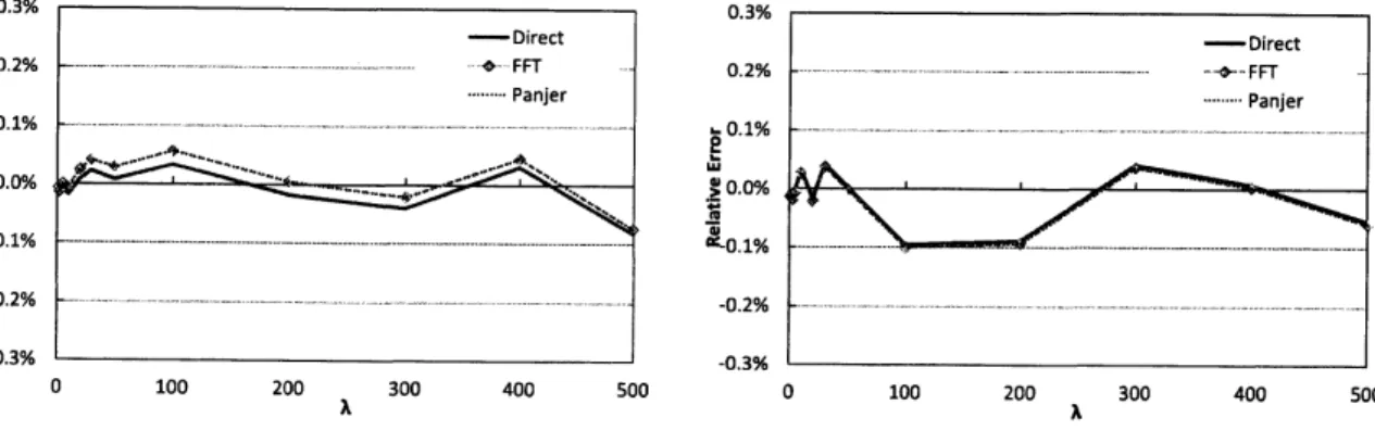
Figures 5-8 show the REs for each method. We can

see

that the REs for most methods are less than 0.2%. Here, the REs in Figure 6 are rather similar. This implies that there

are

non-negligible simulation errors in the OpVaRs themselves because of the fat tail property of

GPD. Therefore, the accuracies of Direct, FFT and Panjer are higher than the ones shown in

Figure 6.

$0 100 200 300 400 500 0 100 200 300 400 500$

A A

Figure 5: Relative error in the case of Figure 6: Relative errorin the

case

of

LND. _GPD.

Table 1 presents the computation times for each method. We

can see

that FFT is rather

fast in each case. On the other hand, Direct is sufficiently fast in the cases of LND and GPD,

whereas itscomputation speedis somewhat lower in the

case

of LIN-EMP and evenlower in the

case

of EMP.

$\mathbb{R}om$the aboveresults, we see that FFT isoneof the most adaptive methods for calculating

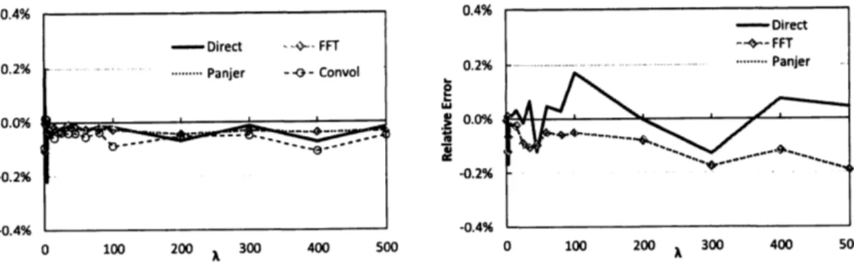
$0$ 100 200 300 400 500

A $0$

$1\infty$ $2\infty$ $3\infty$

A $4\infty$

Figure

7:

Relative

error

inthe

case

of Figure

8:

Relative

error

in the

case

of

EMP. LIN-EMP.

$\lambda$

.

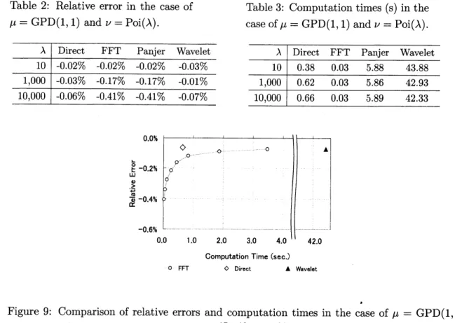
We set _$\nu=$ Poi(A) with $\lambda=1,10^{3},10^{4}$ and GPD(1, 1). Here, we also perform acomparison

with thewavelet transform approach (abbreviated

as

Wavelet) presented in [20].

The results

are

shown in Tables 2-3. We

can see

that the accuracies of FFT and Panjer

are

somewhat lower when $\lambda$ is large, whereas the errors for Direct and Wavelet

are

still less

than 0.1% even when $\lambda=10^{4}$

.

This phenomenon is consistent with the results presented in

[27]. Obviously, the accuracies ofFFT and Panjer can be improved by increasing the number

ofpartitions $M$, which entails

a

longer computation time. Figure 9 shows a comparisonof the

REs and computation times for Direct, FFT and Wavelet, where the number of partitions $M$

for FFT is varied between $2^{17}$ and $2^{24}$

.

We can see that Direct isthe fastest and most accurate

method in this case.

2.4

Concluding

Remarks

As we have seen in Section 2.2, the $MC$ method is slow and not robust in the calculation of

Vaffi of fat-taileddistributions,such

as

OpVaRs. The numerical results in the preceding section imply that FFT is fast and highly accurate inmany

cases

(includingmany realistic situations)

Table 2: Relative error in the case of

$\mu=$ GPD(1,1) and $\nu=$ Poi$(\lambda)$

.

Table 3: Computation times (s) in the

case

of$\mu=$ GPD(1, 1) and $\nu=$Poi$(\lambda)$

.

ComputationTime(sec.)

$-0-$FFT $\Diamond$

Direct A Wavelet

Figure 9: Comparison of relative

errors

and computation times in the case of $\mu=$ GPD(1, 1) and $v=Poi(10,000)$

.

Here, $M$ is taken as $2^{17},2^{18},$

$\ldots,$ $2^{24}.$

On the other hand, to our knowledge, $MC$ is still the de facto standard method in banks,

especially in Japan. Although it is true that the estimated value $VaR_{\alpha}^{MC}(L)$ converges to the

actual value of OpVa$R$withincreasing the number of simulation iterations, the cost of increasing

theaccuracyof the$MC$method without any_{theoretical improvements, suchas}$IS$, is rather high.

Although we could not find the most adaptive method for all cases in practice, the methods

introduced in this paper are sufficiently fast and accurate, and appear to be more reliable than

thesimple$MC$ method. Thus, it mightbe of

use

to_{studythe improvementofanalyticalmethods}

and the application of the $IS$ method in calculating OpVaRs.

3

Asymptotic behavior of OpVa

$R$

and

Sensitivity

Analysis

In the above section, we considered some methods for calculation of OpVaRs. Another notable issue for banks adopting AMA is the verification of their own models since AMA requires not

only the calculation of OpVa$R$, but also the verification ofthe adequacy and robustness of the $mo$del used.

As pointed out in McNeil et al. [19], whereas everyone agrees on the importance of

under-standing operational risk, it is a controversial issue how far

one

should (or can) quantify such risks. Since empirical studies find that the distribution of operational loss has a fat tail (see

the tail of an operational loss distribution is often difficult due to the fact that the

accumu-latedhistoricaldataare insufficient, there

are

various kind of factors of operationalloss, and so

on. Thus we need sufficient verification for the appropriateness and robustness of the model in

quantitative operational riskmanagement.

One of the verification approaches for a risk model is sensitivity analysis (or behaviour

analysis). There

are

a few interpretations for the word “sensitivity analysis”. In this paper,

we use

this word to

mean

the relevance of

a

change of the risk amount with changing input

information (forinstance, added/deletedlossdata

or

changingmodelparameters). There is also

an

advantage in using sensitivity analysis not only to validatethe accuracy of

a

risk model but

also to decideonthe most effective pohcywithregardtothevariablefactors. Thisexaminationof how the variationinthe output ofa model canbe apportioned to different sourcesofvariations

of risk will give an incentive to business improvement. Moreover, sensitivity analysis is also meaningful for

a

scenario analysis. Basel II claims not only to

use

historical internal/extemal data and BEICFs (Business Environment and Intemal Control Factors)

as

input information, but also to use scenario analyses to evaluate low frequency and high severity loss events which cannot be captured by empirical data. As noted above, to quantify operational risk

we

need

to estimate the tail of the loss distribution, so it is important to recognize the impact of

our

scenarios

on

the risk amount.

In this largesection

we

study the sensitivity analysis for the operational risk model from

a

theoretical viewpoint. In particular, we mainly consider the

case

ofadding loss factors. Let $L$

be a random variable which represents the loss amount with respect to the present risk profile and let $S$be

a

random variable of the loss amount caused by an additionallossfactor found by

a

minute investigation

or

broughtabout by expanded business operation. In

a

practical sensitivity

analysisit is alsoimportant toconsider thestatistical effect (theestimation error of parameters,

etc.) for validating an actual risk model, but such an effect should be treated separately. We

focus on the change from apriorrisk amount $\rho(L)$ to aposterior risk amount $\rho(L+S)$, where

$\rho$ is a risk

measure.

Wemainly treat the

case

where the tails ofthe loss distributions

are

regularly varying. We

use$VaR$at the confidence level$\alpha$

as our

risk

measure

$\rho$and

we

study the asymptotic behaviour of

$VaR$

as

$\alphaarrow 1$

.

Our frameworkis mathematicallysimilar tothe studyofB\"ockerandKl\"uppelberg

[6]. They regard $L$ and $S$

as

loss amount variables ofseparate categories (cells) and study the asymptoticbehaviour ofanaggregated loss amount$VaR_{\alpha}(L+S)$

as

$\alphaarrow 1$ (in addition, asimilar

study, adoptinganexpected shortfall (orconditional$VaR$),is foundin BiaginiandUlmer[3]$)$

.

In

contrast,ourpurpose is to estimateamore precise difference between$VaR_{\alpha}(L)$ and$VaR_{\alpha}(L+S)$

andwe obtain different results according to the magnituderelationship ofthe thicknesses of the tailsof$L$ and $S.$

The rest ofthis large section is organized

as

follows. In Section 3.1

we

introduce the frame-work of

our

modeland

some

notation. InSection 3.2 wegive roughestimationsof the asymptotic behaviour of the risk amount $VaR_{\alpha}(L+S)$

.

Ourmain results

are

in Section 3.3 and

we

present a finer estimation of the difference between $VaR_{\alpha}(L)$ and $VaR_{\alpha}(L+S)$

.

Section

3.3.1

treats

results in Section 3.3.1 and we give

some

results when $L$ and $S$ are not independent. One of

these results is related to the study of risk capital decomposition and we study these relations

in Section 3.6. In Section 3.4 wepresent numerical examples ofour results. Section 3.5 presents

some

conclusions. For the proofsof

our

results,

see

[17].

3.1

Settings

We always study a given probability space $(\Omega, \mathcal{F}, P)$. We recall the definition of the $\alpha$-quantile

(Value at Risk): for a random variable $X$ and $\alpha\in(0,1)$, put

$VaR_{\alpha}(X)=\inf\{x\in \mathbb{R} ; F_{X}(x)\geq\alpha\},$

where $F_{X}(x)=P(X\leq x)$ _{is the distribution function of}$X.$

We denote by $\mathcal{R}_{k}$ the set ofregularly varying functions with index _{$k\in \mathbb{R}$}

, that is, $f\in \mathcal{R}_{k}$

if and only if$\lim_{xarrow\infty}f(tx)/f(x)=t^{k}$ for any _$t>0$

.

_{When $k=0$,} a _function $f\in \mathcal{R}_{0}$ is called

slowly varying. For the details ofregularvariation andslowvariation,

see

Binghamet al. [4] and

Embrechts et al. [11]. For

a

random variable $X$,

we

also say $X\in \mathcal{R}_{k}$ when the tailprobability

function $\overline{F}_{X}(x)=1-F_{X}(x)=P(X>x)$ _{is in} $\mathcal{R}_{k}$

.

We mainly treat the

case

of $k<0$

.

In

this case, the mth moment of $X\in \mathcal{R}_{k}$ is infinite for $m>-k$

.

As examples of heavy-tailed

distributionswhich have regularly varying tails, the generalizedPareto distribution (GPD) and

the g-h distribution (see Degen et al. [7], Dutta and Perry [9]) are well-known and are widely used in quantitative operationalrisk management. In particular, GPD plays an important role in extreme value theory (EVT), and it can approximate the excess distributions over a high

threshold of all the commonly used continuous distributions. See Embrechts et al. [11] and McNeil et al. [19] for details.

Let $L$ and$S$ be non-negative random variables and assume

$L\in \mathcal{R}_{-\beta}$and $S\in \mathcal{R}_{-\gamma}$ for

some

$\beta,$$\gamma>0$

.

We call $\beta$ $($respectively,$\gamma)$ the tailindex of$L$ $($respectively, _$S)$

.

$A$tail index represents

the thickness of atail probability. For example, the relation $\beta<\gamma$ means that the tail of$L$ is

fatter than $S.$

We regard $L$ as the total loss amount ofa present risk profile. In the framework of LDA, _$L$

is given

as

(2.1). Ifwe consider a multivariate$mo$del, $L$ is given by $L= \sum_{k=1}^{d}L_{k}$, where $L_{k}$ is

the loss amount variable of the kth operational risk cell $(k=1, \ldots, d)$

.

We

are

aware

_{of such}

formulations, but we do not limit ourselves to such situations in our settings.

The random variable $S$

means

an additional loss amount. We will consider the total loss

amount variable $L+S$ as anew riskprofile. As mentioned above, our interest is in howa prior

risk amount $VaR_{\alpha}(L)$ changes to aposterior one $VaR_{\alpha}(L+S)$

.

3.2

_{Basic Results of Asymptotic Behaviour of}

$VaR_{\alpha}(L+S)$

First wegive a rough estimations of$VaR_{\alpha}(L+S)$

.

We introduce the following condition.

[A] $A$ joint distributionof _{$(L, S)$} satisfies the _{negligiblejoint tail condition}

when

Then

we

have the followingproposition.

Proposition 1 Under condition $[A]$ it holds that

(i)

_If

$\beta<\gamma$, then $VaR_{\alpha}(L+S)\sim VaR_{\alpha}(L)$,

(ii)

_If

$\beta=\gamma$, then$VaR_{\alpha}(L+S)\sim VaR_{1-(1-\alpha)/2}(U)$,

(iii)

_If

$\beta>\gamma$, then$VaR_{\alpha}(L+S)\sim VaR_{\alpha}(S)$

as $\alphaarrow 1$, where the notation $f(x)\sim g(x)$, $xarrow a$ denotes $\lim_{xarrow a}f(x)/g(x)=1$ and $U$ is a

random variable whose distribution

_function

is given by$F_{U}(x)=(F_{X}(x)+F_{Y}(x))/2.$

These results

are

easilyobtained and not novel. Inparticular, when$L$and$S$

are

independent,

this proposition isaspecial

case

of Theorem3.12inB\"ockerandKl\"uppelberg[6] (intheframework of LDA).

In contrast with Theorem 3.12 in B\"ocker and Kl\"uppelberg [6], which implies an estimate

for $VaR_{\alpha}(L+S)$

as

“an aggregation of $L$ and $S$”,

we

review the implications of Proposition 1

from the viewpoint of sensitivity analysis. Proposition 1 implies that when $\alpha$ is close to 1, the

posteriorriskamount isdetermined nearly equally by either risk amountof$L$

or

$S$showingfatter

tail. On theother hand, when the thicknesses ofthe tails is the

same

$(i.e., \beta=\gamma,)$ the posterior

risk amount $VaR_{\alpha}(L+S)$ is given by the $VaR$ of the random variable $U$ and is influenced by

both $L$ and $S$

even

if $\alpha$ is close to 1. The random variable $U$ is the variable determined by

a

faircoin flipping. The risk amount of $U$ is alternated by the tossof coin (head-$L$ and tail-$S$).

3.3

Main

Results

3.3.1 Independent Case

In this section wepresent afinerestimation ofthe differencebetween$VaR_{\alpha}(L+S)$ and$VaR_{\alpha}(L)$

than Proposition 1 when $L$ and $S$

are

independent. The assumption of independence implies

the loss events

are

caused independently by the factors $L$ or $S$

.

In this

case

condition $[A]$ is

satisfied. We prepare additional conditions.

[B] There is

some

$x_{0}>0$ such that $F_{L}$ has

a

positive, non-increasing density function $f_{L}$ on

$[x_{0}, \infty)$, i.e., $F_{L}(x)=F_{L}(x_{0})+ \int_{x_{0}}^{x}f_{L}(y)dy,$ $x\geq x_{0}.$

[C] The function $x^{\gamma-\beta}\overline{F}_{S}(x)/\overline{F}_{L}(x)$converges to some real number $k$ as $xarrow\infty.$

[D] Thesame assertion of $[B]$ holds by replacing $L$ with $S.$

We remark that condition $[B]$ $($respectively, $[D])$ and the monotone density theorem

(Theo-rem 1.7.2

in Bingham et al. [4]$)$ imply $f_{L}\in \mathcal{R}_{-\beta-1}$ $($respectively, $fs\in \mathcal{R}_{-\gamma-1})$

.

The condition $[C]$

seems

a little strict: this implies that $\mathcal{L}_{L}$ and (a constant multiple of)

$\mathcal{L}_{S}$

are

asymptotically equivalent, where $\mathcal{L}_{L}(x)=x^{\beta}\overline{F}_{L}(x)$ and $\mathcal{L}_{S}(x)=x^{\gamma}\overline{F}_{S}(x)$

are

slowly

imples that $\overline{F}_{L}$ and $\overline{F}_{S}$

are

approximated

by GPD, the asymptotic equivalence of $\mathcal{L}_{L}$ and $\mathcal{L}_{S}$

“approximately” holds.

Our maintheorem is the following.

Theorem 1 The following assertions hold as $\alphaarrow 1.$

(i)

_If

$\beta+1<\gamma$, then $VaR_{\alpha}(L+S)-VaR_{\alpha}(L)\sim E[S]$ under$[B].$

(ii)

_If

$\beta<\gamma\leq\beta+1$, then $VaR_{\alpha}(L+S)-VaR_{\alpha}(L)\sim\frac{k}{\beta}VaR_{\alpha}(L)^{\beta+1-\gamma}$under$[B]$ and $[C].$

(iii)

_If

$\beta=\gamma$, then$VaR_{\alpha}(L+S)\sim(1+k)^{1/\beta}VaR_{\alpha}(L)$ under$[C].$

(iv)

_If

$\gamma<\beta\leq\gamma+1$, then $VaR_{\alpha}(L+S)-VaR_{\alpha}(S)$ $\sim$ $\frac{1}{k\gamma}VaR_{\alpha}(S)^{\gamma+1-\beta}$ under $[C]$ and

$[D].$

(v)

_If

$\gamma+1<\beta$, then $VaR_{\alpha}(L+S)-VaR_{\alpha}(S)\sim E[L]$ under $[C]$ and $[D].$

The assertions of Theorem 1 are divided into five cases according to the magnitude rela-tionship between $\beta$ and $\gamma$. In particular, when $\beta<\gamma$, we get different results depending on

whether $\gamma$ is greater than $\beta+1$ ornot. The assertion (i) implies that ifthe tail probability of

$S$ is sufficiently thinner than that of$L$, then the effect of a supplement of $S$ is limited to the

expected loss ($EL$) of $S$

.

In fact, we can also get a similar result to the assertion (i), which we

introduce in Section3.6, when the moment of$S$ isvery small. These results indicate that if

an

additional loss amount $S$ is not so large, we may not have to be nervous about the effect of_a tail event which is raised by $S.$

The assertion (ii) implies that when $\gamma\leq\beta+1$, the difference of a risk amount cannot be

approximated by $EL$ evenif$\gamma>1$

.

Let $l>0$ and $p\in(0,1)$ be such that $P(S>l)=p$_and $l$ is

large enough $(or,$ equivalently, $p is$ small enough) that $VaR_{1-p}(L)\geq VaR_{1-p}(S)=l$

.

Then we

can

interpret the assertion (ii) formally

as

$VaR_{\alpha}(L+S)-VaR_{\alpha}(L)\approx\frac{1}{\beta}(\frac{l}{VaR_{1-p}(L)})^{\gamma}VaR_{\alpha}(L)\leq\frac{1}{\beta}(\frac{l}{VaR_{1-p}(L)})^{\beta}VaR_{\alpha}(L)$

.

(3.2)

Thus it is enough to provide an amount of the right hand side of (3.2) for an additional risk

capital. So, in this case, the information of the pair $(l,p)$ (and detailed information _{about the}

tail of$L$) enables us to estimate the difference conservatively.

When the tail of$S$ has the

same

thickness as that of$L$, we have the assertion (iii). In this

case we see

that by a supplement of$S$, the risk amount is multiplied by _{$(1+k)^{1/\beta}$}

.

Theslower

is the decay speed of $\overline{F}_{S}(x)$, which means the fatter the tail amount variable becomes with an additional loss, the larger is the multiplier $(1+k)^{1/\beta}$

.

Moreover, if $k$ is small,

we

have the

following approximation,

$VaR_{\alpha}(L+S)-VaR_{\alpha}(L)\sim\frac{k+o(k)}{\beta}VaR_{\alpha}(L)$, (3.3)

where $o(\cdot)$ is the Landau symbol (littleo): _{$\lim_{karrow 0}o(k)/k=0$}

.

The relation (3.3) has the same

form

as

assertion (ii), and in this

case

we haveasimilarimplicationas (3.2) by letting$\alpha=1-p$

The

assertions

(iv)$-(v)$

are

restated

consequences

of the

assertions

$(i)-$(ii). In these cases,

$VaR_{\alpha}(L)$ istoo much smaller than$VaR_{\alpha}(L+S)$ and $VaR_{\alpha}(S)$,

so we

needtocompare$VaR_{\alpha}(L+$ $S)$ with $VaR_{\alpha}(S)$

.

In estimating the posterior risk amount $VaR_{\alpha}(L+S)$, the effect of the tail

index$\gamma$ of$S$is significant. Weremarkthatwecan replace$VaR_{\alpha}(S)$with

$k^{1/\gamma}aR_{\alpha}(L)^{\beta/\gamma}$ when

either$x^{\beta}F_{L}(x)$

or

$x^{\gamma}F_{S}(x)$ converges to

some

positive number (see [17]).

ByTheorem 1,we

see

thatthe smaller is the tail index$\gamma$, the

more

preciseis the information

which

we

needabout the tail of$S.$

3.3.2 Consideration of Dependency Structure

In the previous section

we

assumed that $L$ and $S$ were independent, since they

were

caused

by different loss factors. However, huge losses often happen due to multiple simultaneous loss

events. Thus it is important to

prepare

a

risk capital considering

a

dependency structure

be-tween loss factors. Basel II states that “scenario analysisshouldbeused to

assess

the impactof

deviations from the correlation assumptions embedded in the bank’s operational risk

measure-ment framework, in particular, to evaluate potential losses arising from multiple simultaneous

operational risk loss events” in paragraph675 of Basel Committee onBanking Supervision [2]. In this section we consider the

case

where $L$ and $S$

are

not necessarily independent, and

present generalizations of Theorem 1$(i)-$(ii). Let $L\in \mathcal{R}_{-\beta}$ and $S\in \mathcal{R}_{-\gamma}$ be random variables

for

some

$\beta,$$\gamma>0$

.

We only consider the

case

of $\beta<\gamma$

.

By using the fact that $(\mathbb{R}^{2}, \mathcal{B}(\mathbb{R}^{2}))$ is

a standard Borel spaceand Theorem

5.3.19

in Karatzas and Shreve [16], we

see

that there is

a

regular conditionalprobabilitydistribution$p$ (respectively, q) : $[0, \infty)\cross\Omegaarrow[0,1]$ with respect

to $\sigma(L, S)$ given $S$ $($respectively, $L)$

.

We define the function $F_{L}(x|S=s)$ by $F_{L}(x|S=s)=$

$p(s, \{L\leq x\})$

.

We

see

that the function$F_{L}(x|S=s)$ satisfies

$\int_{B}F_{L}(x|S=s)F_{S}(ds)=P(L\leq x, S\in B)$

for each Borel subset $B\subset[0, \infty)$

.

We preparethe followingconditions.

[E] There is

some

$x_{0}>0$ such that $F_{L}(\cdot|S=s)$ has apositive, non-increasing and continuous

density function $f_{L}(\cdot|S=s)$ on $[x_{0}, \infty)$ for $P(S\in\cdot)$-almost all $s.$

[F] It holds that

$ess\sup_{s\geq 0}\sup_{t\in K}|\frac{f_{L}(tx|S=s)}{f_{L}(x|S=s)}-t^{-\beta-1}|arrow 0, xarrow\infty$ (3.4)

for any compact set $K\subset(0,1]$ and

$\int_{[0,\infty)}s^{\eta}\frac{f_{L}(x|S=s)}{f_{L}(x)}F_{S}(ds)\leq C, x\geq x_{0}$ (3.5)

for

some

constants $C>0$ and$\eta>\gamma-\beta$, where

ess

sup is the $L^{\infty}$

-norm

under the

measure

$P(S\in\cdot)$.

We notice that the condition $[E]$ includes the condition $[B]$

.

Under these conditions we have $P(L>x, S>x)\leq Cx^{-\eta}\overline{F}_{L}(x)$ and then the condition $[A]$ is also satisfied.

Let $E[\cdot|L=x]$ bethe expectation under the probability

measure

$q(x, \cdot)$

.

Underthe condition

[E], we seethat for each $\varphi\in L^{1}([0, \infty), P(S\in\cdot))$

$E[\varphi(S)|L=x]=\int_{[0,\infty)}\varphi(s)\frac{f_{L}(x|S=s)}{f_{L}(x)}F_{S}(ds)$ (3.6)

for $P(L\in\cdot)$-almost all $x\geq x_{0}$

.

Wedonot distinguish the left hand side and the right hand side

of (3.6). The left hand side of (3.5) isregarded as $E[S^{\eta}|L=x].$

The conditions [E] and [F] seem to be a little strong, but we can construct a non-trivial

example. Please refer to [17] for details.

Now we present the following theorem.

Theorem 2 Assume $[E]$ and$[F]$.

If

$\beta+1<\gamma$, then

$VaR_{\alpha}(L+S)-VaR_{\alpha}(L) \sim E[S|L=VaR_{\alpha}(L)], \alphaarrow 1$. _(3.7)

Therelation (3.7) gives asimilar indication of (5.12) in Tasche [30]. The right hand side of (3.7) has the

same

form

as

the so-called component $VaR$:

$E[S|L+S=VaR_{\alpha}(L+S)]=\frac{\partial}{\partial\epsilon}VaR_{\alpha}(L+\epsilon S)|_{\epsilon=1}$ (3.8)

under some suitable mathematical assumptions. In Section 3.6 we study the details. We can

replace the right hand side of (3.7) with (3.8) by afew $mo$difications ofour assumptions:

$[E‘]$ The

same

condition

as

$[E]$ holds by replacing $L$ with$L+S.$

$[F’]$ The relations (3.4) and (3.5) hold by replacing $L$ with $L+S$ and by setting _{$K=[a, \infty)$}

for any $a>0.$

Indeed, our proofalso works upon replacing $(L+S, L)$ with $(L, L+S)$

.

3.4

Numerical

Examples

In this section we confirm numerically our main results for typical examples in the standard

LDA framework. Let $L$ and $S$ be given by the following compound Poisson variables: _$L=$

$L^{1}+\cdots+L^{N},$ $S=S^{1}+\cdots+S^{\tilde{N}}$_{, where} $(L^{i})_{i},$ $(S^{i})_{i},$$N,\tilde{N}$ are independent random variables

and $(L^{i})_{i},$ $(S^{i})_{i}$

are

each identically distributed. The variables _$N$ and $\tilde{N}$mean the frequency of

loss events, and the variables $(L^{i})_{i}$ and $(S^{i})_{i}$ mean the severity of each loss event. We assume

that $N\sim$ Poi$(\lambda_{L})$ and $\tilde{N}\sim$ Poi$(\lambda_{S})$ for

some

$\lambda_{L},$$\lambda_{S}>0$

.

For severity,

we

assume

that $L^{i}$

follows GPD$(\xi_{L}, \sigma_{L})$ with_{$\xi_{L}=2,$$\sigma L=10,000$} andset _{$\lambda_{L}=10$}

.

We also assumethat $S^{i}$ follows GPD$(\xi_{S}, \sigma s)$ and $\lambda_{S}=10$

.

We set the parameters $\xi s$ and $\sigma_{S}$ in each cases appropriately. We

remark that $L\in \mathcal{R}_{-\beta}$ and $S\in \mathcal{R}_{-\gamma}$, where$\beta=1/\xi_{L}$ and$\gamma=1/\xi s$

.

Moreover the condition $[C]$

is satisfied with

Hereweapply thedirectapproachintroducedin Section

2.3.1

tocalculate numerically.

Unless otherwise noted,

we

set $\alpha=0.999$

.

Then the value ofthe prior risk amount$VaR_{\alpha}(L)$ is

5.01

$\cross 10^{11}.$

3.4.1 The Case of $\beta+1<\gamma$

First we consider the

case

of Theorem 1(i). We set $\sigma s=10,000$

.

The result is given in Table 4,

where

$\Delta VaR=VaR_{\alpha}(L+S)-VaR_{\alpha}(L)$, Error$= \frac{Approx}{\Delta VaR}-1$ (3.10)

and Approx$=E[S].$

Although the absolute value of the error becomes a little large when $\gamma-\beta$ is

near

1, the

difference between the $VaRs$ is accurately approximated by$E[S].$

Table 4: The

case

of$\beta+1<\gamma$

.

Table 5: The

case

of$\beta<\gamma\leq\beta+1.$

Table 6: The

case

of$\beta=\gamma.$

3.4.2 The Case of$\beta<\gamma\leq\beta+1$

This

case

corresponds to Theorem 1(ii). As inSection3.4.1, wealso set $\sigma_{S}=10,000$

.

The result isgivenas Table 5, where Approx $=kVaR_{\alpha}(L)^{\beta+1-\gamma}/\beta$ and theerror is the same as (3.10). We

see that the accuracy is lower when $\gamma-\beta$ is close to 1 or $0$

.

Even in these cases, the error

approaches $0$ by letting $\alphaarrow\infty$ (see [17]).

3.4.3 The Case of$\beta=\gamma$

Inthis section

we

set $\xi_{S}=2(=\xi_{L})$

.

We apply Theorem 1(iii). We compare the values of $\Delta VaR$

and Approx$=((1+k)^{\xi_{L}}-1)VaR_{\alpha}(L)$ in Table 6, where theerroris the the

same as

(3.10). We see that they

are

very close.

3.4.4 The Case of$\beta>\gamma$

Finallywe treat the

case

of Theorem 1(iv). We set $\sigma s=100$

.

In this

case

$VaR_{\alpha}(L)$ is too much

smaller than $VaR_{\alpha}(L+S)$, so we compare the values of$VaR_{\alpha}(L+S)$ and

Approx$= VaR_{\alpha}(S)+\frac{1}{k\gamma}VaR_{\alpha}(S)^{\gamma+1-\beta}.$

The result is in Table 7. We

see

that the error $(=$ Approx$/VaR_{\alpha}(L+S)-1)$ tends to _become

smaller when$\xi_{S}$ is large.

Table 7 also indicates that the supplement of $S$ has a quite significant effect on the risk

amount when the distribution of $S$ has

a

fat tail. For example, when _{$\xi s=3.0$}, the value of

$VaR_{\alpha}(L+S)$ is

more

than90 times $VaR_{\alpha}(L)$ and is heavily influenced by the tail of$S$

.

We see

that a littlechange of$\xi_{S}$ may cause ahuge impact onthe risk model.

In our example we do not treat the case of Theorem 1(v), however we also have a similar

implication in this case.

3.5

Concluding Remarks

We introduced the theoretical framework of sensitivity analysis for quantitative operational

risk management. Concretely speaking, we investigated the impact on the risk amount $(VaR)$

arising from addingthe loss amount variable $S$ to the present loss amount variable $L$ when the

tail probabilites of $L$ and $S$

are

regularly varying $(L\in \mathcal{R}_{-\beta}, S\in \mathcal{R}_{-\gamma} for some \beta, \gamma>0)$

.

The

result depends on the magnitude relationship of$\beta$ and$\gamma$

.

One of these implications is that we

must pay

more

attention to the form of the tail of$S$ when$S$has the fatter tail. Moreover, when

$\gamma>\beta+1$, the difference between the _{prior $VaR$ andthe posterior $VaR$is approximated by the}

component $VaR$ of$S$ (in particular by $EL$ of$S$ if$L$ and $S$are independent).

We have mainly treated the case where $L$ and $S$ are independent except for a few

cases

in

Section 3.3.2. As related study for dependent case, B\"ocker _{and Kl\"uppelberg [5] invokes a} L\’evy

copulato describe the dependency and givesan asymptotic estimate ofFr\’echet bounds of total

$VaR$. To deepen andenhance our_{study inmore generalcaseswhen}$L$ and $S$have adependency

structure is one of the directions ofour future work.

3.6

Appendix;

The Effect

of

a

Supplement of Small

Loss Amount

Inthis section we treat another version of Theorem 1 (i) and Theorem 2(i). We do not

assume

that the random variables are regularly varying but that the additional loss amount variable is very small. Let $L,\tilde{S}$ be non-negative

random variables and let $\epsilon>0$. We define a random

variable $S_{\epsilon}$ by $S_{\epsilon}=\epsilon\tilde{S}$

.

Weregard $L$ $($respectively, $L+S_{\epsilon})$

as

the prior (respectively, posterior)

loss amount variable and consider the limit ofthe difference between thepriorandposterior$VaR$

by taking $\epsilonarrow 0$

.

Instead of making assumptions of regular variation, we make “Assumption

$(S)$” in Tasche [30]. Then Lemma 5.3 and Remark 5.4 _{in Tasche [30] imply}

By (3.11),

we

have

$VaR_{\alpha}(L+S)-VaR_{\alpha}(L)=E[S|L=VaR_{\alpha}(L)]+o(\epsilon)$, (3.12)

where

we

simply put $S=S_{\epsilon}$

.

In particular, if$L$ and $S$

are

independent, then

$VaR_{\alpha}(L+S)-VaR_{\alpha}(L)=E[S]+o(\epsilon)$

.

Thus the effect of a supplementof the additional loss amount variable $S$ is approximated by its

component $VaR$

or

$EL$

.

So the assertions of Theorem 1(i) and Theorem 2(i) also hold in this case.

The concept of the component $VaR$ is related to the theory of risk capital decomposition

(or risk capital allocation). Let

us

consider the

case

where $L$ and $S$

are

loss amount variables

and where the total loss amount variable is given by $T(w_{1}, w_{2})=w_{1}L+w_{2}S$ with

a

portfolio

$(w_{1}, w_{2})\in \mathbb{R}^{2}$ such that _{$w_{1}+w_{2}=1$}

.

We try to calculate the risk contributions for the total

risk capital $\rho(T(w_{1}, w_{2}))$, where $\rho$ is arisk

measure.

One of the ideas is to apply Euler’s relation

$\rho(T(w_{1}, w_{2}))=w_{1}\frac{\partial}{\partial w_{1}}\rho(T(w_{1}, w_{2}))+w_{2}\frac{\partial}{\partial w_{2}}\rho(T(w_{1}, w_{2}))$

when $\rho$ islinear homogeneous and $\rho(T(w_{1}, w_{2}))$ is differentiable with respect to$w_{1}$ and $w_{2}$

.

In

particular we have

$\rho(L+S)=\frac{\partial}{\partial u}\rho(uL+S)|_{u=1}+\frac{\partial}{\partial u}\rho(L+uS)|_{u=1}$ (3.13)

and the second term in the right handside of (3.13) is regarded

as

the risk contribution of $S.$

As in early studies in the

case

of $\rho=VaR_{\alpha}$, the

same

decomposition

as

(3.13) is obtained in

Garman [12] and Hallerbach [13] and the risk contribution of $S$ is called the component $VaR.$

The consistency of the decomposition of (3.13) has been studied from several points of views

(Denault [8], Kalkbrener [15], Tasche [30], and soon). In particular, Theorem4.4 inTasche [30] implies that the decomposition of (3.13) is “suitable for performance measurement” (Definition

4.2 of Tasche [30]$)$

.

Although manystudies assumethat $\rho$ is acoherent risk measure, the result

of Tasche [30] also applies to the

case

of$\rho=VaR_{\alpha}.$

Another approachtowards calculatingthe risk contribution of$S$istoestimate the difference

of the risk amounts $\rho(L+S)-\rho(L)$, which is called the marginal risk capital–see Merton

and Perold [21]. $(When \rho=VaR_{\alpha}, it is$ called $a$marginal $VaR.)$ This is intuitively intelligible,

whereasanaggregation ofmarginal risk capitals is not equal to the total riskamount $\rho(L+S)$

.

Therelation (3.12)givesthe equivalence between the marginal$VaR$and the component$VaR$

when $S(=\epsilon\tilde{S})$ is very small. Theorem 2(i) implies that the marginal $VaR$ and the component

$VaR$

are

also (asymptotically) equivalentwhen $L$ and $S$have regulary varying tails and the tail

of$S$is sufficiently thinner than that of$L.$

References

[1] A. Balkema and L. de Haan, Residual Life Time at Great Age, Ann. Prob. 2(1974), pp.

[2] Basel

Committee on

Banking _{Supervision, International Convergence of Capital}

Measure-ment and Capital

Standards:

A Revised Framework, Bank of Intemational Settlements,

Available from http:$//www.bis.org/$, 2004.

[3] F. Biagini and S. Ulmer, Asymptoticsfor OperationalRiskQuantifiedwith Expected Short-fall,

Astin

Bull., 39(2008), pp.

735-752.

[4] N. H. Bingham, C. M. Goldie and J. L. Teugels, Regular Variation, Cambridge University Press, 1987.

[5] C. B\"ocker and C. Kl\"uppelberg, Operational VaR: A Closed-Form

Approximation,

Risk,

18-12(2005), pp.

90-93.

[6] C. B\"ocker and C. Kl\"uppelberg, Multivariate Models for Operational Risk, Quant. Finance,

$10-8(2010)$, pp. 855-869.

[7] M. Degen, P. Embrechts and D. D. Lambrigger, The Quantitative Modeling of Operational Risk: Betweeng-and-h and EVT, Astin Bull., $37-2(2006)$, pp.

265-291.

[8] M. Denault, Coherent Allocationof Risk Capital, Journal ofRisk, 4-1(2001),pp. 1-34.

[9] K. Dutta and J. Perry, A Tale of Tails: An Empirical Analysis of Loss Distribution Models

for Estimating Operational Risk Capital, Working papers of the Federal Reserve Bank of

Boston,

Available

fromhttp:$//www.bos.frb.org/$, 2006. No. 06-13, 2006.

[10] P. Embrechtsand M.Frei, Panjer RecursionversusFFTfor Compound Distributions, Math-ematical Methods ofOperations Research, $69-3(2009)$, pp. 497-508.

[11] P. Embrechts, C. Kl\"uppelberg and T. Mikosch, Modelling Extremal Events, Springer,

Berlin,

2003.

[12] M. _{Garman, Taking VaR to} Pieces, Risk, $10-10(1997)$, pp. _70-71.

[13] W.Hallerbach, DecomposingPortfolio Value-at-Risk: A General Analysis, Journal ofRisk,

$5-2(2003)$, pp. 1-18.

[14] J. Jang and J. H. Jho, Asymptotic Super(sub)additivity of Value-at-Risk of Regularly

Varying _{Dependent Variables, Preprint, MacQuarie University, Sydney, 2007.}

[15] M. Kalkbrener, An AxiomaticApproach to Capital Allocation, Mathematical Finance,

15-3(2005), pp.

425-437.

[16] I. Karatzas and S. E. Shreve, Brownian Motion and Stochastic Calculus 2nd. edition,

Springer, New York, 1991.

[17] T. Kato, Theoretical Sensitivity Analysis for Quantitative Operational Risk Management, Intellectual Archive, $1-2(2012)$, pp. 99-115.

[18] X. Luo and P. V. Shevchenko, Computing Tails of Compound Distributions Using Direct

NumericalIntegration, The Journal of Computational Finance, $13-2(2009)$, pp.

73-111.

[19] A. J. McNeil, R. Frey and P. Embrechts, QuantitativeRisk Management: Concepts,

Tech-niques and Tools, Princeton University Press, 2005.

[20] K. Ishitani and K. Sato, Wavelet $\mathscr{Z}B$を$fflv\backslash$たオへ$\circ\triangleright$–_シ$\exists^{-\gamma_{J\triangleright)}}1$ スクの

ne

$ffi^{;}\mathfrak{X}_{\overline{p}^{\backslash }}^{\equiv}\ovalbox{\tt\small REJECT} \mathbb{H}\mathfrak{B}\not\in,$ $\ovalbox{\tt\small REJECT} 36\square ^{\backslash }\sqrt[\backslash ]{}*7\backslash ^{\backslash }$

イ$-\lambda_{R}^{\infty}\#ffi\ovalbox{\tt\small REJECT}$ (2012).

[21] R. C. Merton and A. F. Perold, Theory of Risk Capital in Financial Firms, Journal of

Applied Corporate Finance, $5-1(1993)$, pp.

16-32.

[22] M. Moscadelli, The Modelling of Operational Risk: Experience with the Analysis of the

Data Collected by the Basel Committee, Technical report of Banking Supervision

Depart-ment, Banca d’Italia, 517, Available from http:$//www.$bancaditalia.$it/$, 2004.

[23] T. Ooura and M. Mori, The Double Exponential Formula for Oscillatory Functions Over

the Half Infinite Interval, J.Comput. Appl. Math. 38(1991), pp. 353-360.

[24] T. Oouraand M. Mori, A Robust Double ExponentialFormula for Fourier TypeIntegrals,

J.Comput. Appl. Math. 112(1999), pp. 229-241.

[25] J. Pickands, Statistical Inference Using Extreme Order Statistics, Ann. Stat. 3(1975), pp.

119-131.

[26] M. Pritsker, Evaluating Value at Risk Methodologies: Accuracy

versus

Computational

Time, Journalof Financial Services Research, 12(1997), pp.

201-242.

[27] P.V. Shevchenko, Calculation ofAggregate LossDistributions, TheJournal ofOperational

Risk, $5-2(2010)$, pp. 3-40.

[28] H. Takahashi and M. Mori, Quadrature Formulas Obtained by Variable Transformation,

Numer. Math., 21(1973), pp. 206-219.

[29] H. Takahashiand M. Mori, DoubleExponentialFormulas for NumericalIntegration, Publ.

RIMS Kyoto Univ. 9(1974), pp.

721-741.

[30] D. Tasche, Risk Contributions and Performance Measurement, Working Paper, Center for Mathematical Sciences, Munich University of Technology, Available from

http://www-$m4.ma.tum.de/$, 2000.

[31] Wynn P., On aDevice for Computing the $e_{m}(s_{n})$ banformation, MathematicalTables and

Other Aids to Computation, 10(1956), pp. 91-96.

Division of Mathematical Science forSocial Systems, Graduate School of Engineering Science

OsakaUniversity, Toyonaka560-8531, Japan

$E$-mail address: kato@sigmath.es.osaka-u.ac.jp