Toda-type Cellular Automaton and its $N$-soliton Solution(Discretizations of Integrable Systems : Theory and Applications)

Toda-type

Cell.u.lar

Automaton

$.\mathrm{a}$

nd

its

N-s..o

$1.\mathrm{i}\mathrm{t}\mathrm{o}.\mathrm{n}$ :

:

$r$

Solution

J.

_Mat..s

ukidaira

$\mathrm{a}$

,

J.

$\mathrm{S}\mathrm{a}\mathrm{t}_{\mathrm{S}\mathfrak{U}\mathrm{m}}\mathrm{a}^{\mathrm{b}}$

,

D.

$\mathrm{T}\mathrm{a}\mathrm{k}\mathrm{a}\mathrm{h}\mathrm{a}\mathrm{S}\mathrm{h}\mathrm{i}^{\mathrm{a}}.\backslash$

’

T.

Tok,i

hiro

$\mathrm{b}$

and

M.

Toriib

a _Department

_of

_{Applied Mathematics and Informatics, Ryukoku University, Seta,}

Ohtsu 520-21, Japan $\mathrm{b}$

.

G

_raduate.

School

_of

.M

athematical Sciences, University

_of

Tokyo, Meguro-ku, Tokyo 153, Japan

Abstract

In this letter,weshowthat the cellular automaton proposed by twoofthe authors

(D.Tand $\mathrm{J}.\mathrm{M}$) is obtained from the discrete Toda lattice equation throughaspecial

limiting procedure. Also by applying a similar kind of limiting procedure to the

$N$-soliton solution of the discrete Toda lattice equation, we obtain the N-soliton

solution for this cellular automaton.

Keywords: Soliton; Discrete; Cellular Automaton; Nonlinear; Toda Lattice

The phenomena we observe in nature have been described in many ways. Among several methods to analyze the behavior of nature, $\mathrm{d}_{1}^{\mathrm{x}\mathrm{f}\mathrm{f}\mathrm{i}\mathrm{a}1}\mathrm{e}\mathrm{r}\mathrm{e}\mathrm{n}\mathrm{t}$

equa-tions have been traditionallythemost powerful and often used. However many systems in the fieldsof biology, statistical physics, etc., aredifficult to describe using differential equations. These systems

are

rather easy to deal with using discrete methods, such

as

discrete equations, coupled map lattices and cellular automata$(\mathrm{C}\mathrm{A}’ \mathrm{s})[\mathrm{l}\mathrm{J}$.

Due to the enormous growth ofcomputer power in recent years, we have been

able to analyze these discrete systems even though they have large degrees

of freedom and strong nonlinearity. Among them, CA’s

are

most suited for computer simulation because all of the variables are discrete, including field variables, and round off

error

does not occur. Therefore CA’s

are

extensively studied and various statistical results are obtained, though traditional meth-ods used in differential calculus

_coul.d

not have been $\mathrm{a}\mathrm{p}$

.plied

due to

th.e

strong

nonlinearity.

On the other hand, in the field of

noniinear

$\mathrm{p}\mathrm{h}\mathrm{y}\mathrm{S}\dot{\mathrm{i}}_{\mathrm{C}}\mathrm{S}$, soliton theory has

years and has been applied to several fields: hydrodynamics, plasma physics, optical physics and

so on.

$\mathrm{M}_{0}\mathrm{f}\mathrm{e}\mathrm{o}- \mathrm{v}\mathrm{e}\mathrm{r}$ recent development ofsoliton theory tells

us

it

can

be also applicable to discrete $\mathrm{e}\mathrm{q}\mathrm{u}\mathrm{a}\mathrm{t}\mathrm{i}\mathrm{o}\mathrm{n}\mathrm{S}[2-6]$

.

The notion of soliton CA’s

was

first introduced by Park et $\mathrm{a}1[7]$. After this

work, soliton-like structures have been found in several CA’s and attempts

to apply soliton theory to CA’s have been made by several groups [8-11]. However direct relation of CA to soliton equations has not been clear.

Recently we proposed

a

general method to obtain CA’s from discrete soliton

equations through

a

limiting$\mathrm{p}\mathrm{r}\mathrm{o}\mathrm{c}\mathrm{e}\mathrm{d}\mathrm{u}\mathrm{r}\mathrm{e}[12]$

.

By using this method,

we

clarified

the relation between the CA which

was

proposed by two of the authors $(\mathrm{D}.\mathrm{T}$.

and $\mathrm{J}.\mathrm{S}$

.

)$[13]$ and the Korteweg de-Vries equation. This

is

our

answer

to

one

of the unsolved problems listed in the paper of$\mathrm{W}\mathrm{o}\mathrm{l}\mathrm{f}\mathrm{r}\mathrm{a}\mathrm{m}[14]$.

In this letter, we apply this method to the Toda lattice equation. We show that the $\mathrm{C}\mathrm{A}$, which is proposed in the previous

$\mathrm{p}\mathrm{a}\mathrm{p}\mathrm{e}\mathrm{r}[15]$, is obtained from the

discrete Toda lattice equation through the limitingprocedure. Also

we

obtain

$N$-soliton solutions of this CA from those of the discrete Toda lattice equation.

The starting point is the discrete Toda lattice equation which was introduced by $\mathrm{H}\mathrm{i}\mathrm{r}\mathrm{o}\mathrm{t}\mathrm{a}[16]$,

$\log(1+V_{n}^{t}+1)-2\log(1+Vt)n\mathrm{l}+\mathrm{o}\mathrm{g}(1+V-1)n$

$=\log(1+\delta 2Vt)n+1-2\log(1+\delta 2V_{n}t)+\log(1+\delta 2V_{n-1}t).-$ (1)

By introducing $V_{n}^{t}=e^{U_{n}^{\iota}}-1$,

we

obtain

$U_{n}^{t+-}1-2U_{n}t+U_{n}^{t1}$

$=\log(1+\delta 2(eU_{n+}t1-1))-2\log(1+\delta 2(e^{U}n-1))t+\log(1+\delta 2(e^{U_{n}}-1-1)e)$ .

(2) One

can

easily _{obtain the continuous Toda lattice equation,}

$\frac{d^{2}r_{n}}{dt^{2}}--e^{r_{n+}}1-2en+e^{r_{n-1}}’$, ₍₃₎

from $\mathrm{E}\mathrm{q}.(2)$ by the relation $U_{n}^{t}=r_{n}(\delta t)$ and taking $\deltaarrow 0$.

The $N$-soliton solution of$\mathrm{E}\mathrm{q}.(2)$ is given by

with

$f_{n}^{t}= \sum_{0\mu_{i}=1},\exp[\sum_{1i=}^{N}\mu i\xi i+\sum_{<ij}^{(N)}\mu_{i}\mu jA_{i}j]$, (5)

where the difference operator $\triangle_{n}^{2}$ on $F_{n}$ is defined by

$\triangle_{n}^{2}F_{n}=F_{n+}1^{-}2F_{n}+F_{n-1}$, (6)

and

$\xi_{i}=P_{i}n-\Omega_{i}t+\xi_{i}0$, (7)

$\delta^{-1}\sinh(\Omega i/2)=\sigma_{i}\sinh(P_{i}/2)$, (8)

$\exp A_{ij}=\frac{\sigma_{i}\sigma_{j}-\cosh(\frac{P_{i}+\Omega_{i}-P\mathrm{j}-\Omega \mathrm{j}}{2})}{\sigma_{i}\sigma_{j}-\cosh(\frac{P_{i}+\Omega_{i}+P_{\mathrm{j}}+\Omega_{j}}{2})}$ , (9)

$\sigma_{i},$ $\sigma_{j}=1$ or $-1$

.

(10)

Here $\xi_{i}^{0}$ and $P_{i}(i=1,2, \cdots, N)$

are

arbitrary parameters, and _{$\sum_{\mu:=0,1}$} denotes

the summation

over

all terms obtained by replacing each $\mu_{i}$ by $0$

or

1 and

$\sum_{i>}^{(N)}j$ denotes the summation

over

all possible pairs chosen from $N$ elements.

Now we introduce a positive parameter $\epsilon$ defined by

$\delta=e^{-\frac{L}{2\epsilon}}$

where $L$ is a

positive integer, and set $U_{n}^{t}=u_{n}^{t}/\epsilon$. Then noticing the fact

$\lim_{\epsilonarrow+0}\epsilon\log(1+e^{\frac{X}{\epsilon}})=\max(0, X)=\{$

$X$ if $X\geq 0$,

$0$ otherwise,

(11)

we obtain from $\mathrm{E}\mathrm{q}.(2)$ in the limit $\epsilonarrow+0$

$u_{n}^{t+1}-2u^{t}+u^{t}nn-1$

$= \max(\mathrm{o}, u_{n+1}^{t}-L)-2\max(\mathrm{o}, u^{t}-nL)+\max(\mathrm{O}, u_{n-1}-Lt)$, (12)

where the equivalent equation

was

proposed inthe previous $\mathrm{p}\mathrm{a}\mathrm{p}\mathrm{e}\mathrm{r}[15]$

.

$\mathrm{E}\mathrm{q}.(12)$

thus obtained is considered to be

a

Toda-type $\mathrm{C}\mathrm{A}$, which shares

common

algebraic properties with Toda lattice equation

as

shown below. (Here

we use

the term CAin

an

extended meaning, that is,

we

allow the dependent variable

$u_{n}^{t}$ to take values in all integers.)

Let

us

look at whether the $N$-soliton solution

can

survive by this limiting

procedure. The one-soliton solution of$\mathrm{E}\mathrm{q}.(2)$ is expressed by

where

$\sinh(\Omega/2)=\sigma\delta\sinh(P/2)$, (14)

$\sigma=1$ or–l, (15)

Here

we

set $P=p/\epsilon,$ $\Omega=\omega/\epsilon$, and $\xi^{0}=\eta^{0}/\epsilon$, and obtain

$u_{n}^{t}=\epsilon\Delta_{n}2\log(1+e\epsilon)\infty n-\omega t+^{0}$

. (16)

Taking $\epsilonarrow+0$, Eqs.(16) and (14), respectively, become

$u_{n}^{t}= \Delta_{n}2\max(\mathrm{o},pn-\omega t+\eta^{0})$, (17)

$=\{$

$0$ if $n \underline{<}\frac{\omega t-\eta^{0}}{p}-1$,

$\mathrm{u}_{\{p}p(n+1)-\omega t+\eta 0p\}$ if $\frac{\omega t-\eta^{0}}{p}-1\leq n\leq\frac{\omega t-\eta^{0}}{p}$,

$-_{p}^{\mathrm{p}1}\{p(n-1)-\omega t+\eta\}0$ if $\frac{\omega t-\eta^{0}}{p}\leq n\leq\frac{\omega t-\eta^{0}}{p}+1$,

$0$ if $n \geq\frac{\omega t-\eta^{0}}{p}+1$, (18) .. and $\omega=\{$ $\sigma(p-L)$ if $p>L$, $0$ $\mathrm{i}\mathrm{f}-L\leq p\leq L$, $-\sigma(-p-L)$ if $p<-L$, (19) $= \sigma(\max(\mathrm{o},p-L)-\max(0, -p-L))$. ₍₂₀₎

This is the one-soliton solution of$\mathrm{E}\mathrm{q}.(12)$, which is identical to the one shown

in [15] if we take $p,$ $\eta^{0}$

as

integers and $L=1$. It is easy to

see

the speed and

the maximum amplitude of soliton is expressed by $\omega/p$ and $|p|$ respectively.

By setting $P_{i}=p_{i}/\epsilon,$ $\Omega_{i}=\omega_{i}/\epsilon,$$\xi_{i}^{0}=\eta_{i}^{0}/\epsilon,$ _{$A_{ij}=a_{ij}/\epsilon$} and noticing the fact

$\lim_{\epsilonarrow+0}\epsilon\log(\sum e^{\frac{X}{\epsilon}})\dot{\mathrm{A}}=\mathrm{m}\mathrm{a}\mathrm{x}i=1M(X1, X2, \ldots,x_{M}-1, x_{M})$ , (21)

we

also obtain the $N-\mathrm{s}\mathrm{o}.1.\mathrm{i}\mathrm{t}0\mathrm{n}\mathrm{s}\mathrm{o}\mathrm{l}\mathrm{u}\mathrm{t}:\backslash \cdot \mathrm{i}_{\mathrm{o}\mathrm{n}}$ in the

limi.t

_{$\epsilonarrow.+0$}

$u_{n}^{t}=\Delta_{n^{\beta_{n}}}2t$,

with

$\rho_{n}^{t}=\max_{1\mu i=0},[\sum_{1i=}^{N}\mu_{i}\eta_{i}+\sum_{<ij}^{(N)}\mu_{i}\mu ja_{i}j]$, (23)

where $\eta_{i}=p_{i}n-\omega it+\eta_{i}^{0}$, and

$\omega_{i}=\sigma_{i}(\max(0,pi-L)-\max(\mathrm{o}, -pi^{-}L))$, (24)

$a_{ij}=\{$

$-2 \min(|p_{i}|, |p_{j}|)+L$, if $\sigma_{i}=-1$ and $\sigma_{j}=-1$,

(25)

$\max(\min(p_{i}+\omega_{i}, -p_{j}-\omega_{j}),$ $\min(-pi-\omega_{i,p_{j}}+\omega_{j}))$, $\mathrm{o}\mathrm{t}\mathrm{h}\dot{\mathrm{e}}\mathrm{r}\mathrm{W}\mathrm{i}\mathrm{S}\mathrm{e}$.

(Forthe precise derivation of$\mathrm{E}\mathrm{q}.(25)$,

see

Appendix.) Here

$p_{i},$$\eta_{i}^{0}$

are

arbitrary

parameters, and$\max_{\mu_{i}=0,1}[x(\mu i)]$ denotes themaximum valuein $2^{N}$ possiblevalues

of$X(\mu_{i})$ obtained by replacing each $\mu_{i}$ by $0$

or

1. This solution expresses the

interaction of solitons

as

shown in [15] ifwe take$p_{i},$$\eta_{i}^{0}$

as

integers and $L=1$

.

Let

us see how the phaseshiftof$\mathrm{s}\mathrm{o}\mathrm{l}\mathrm{i}\mathrm{t}_{0}\mathrm{n}.\mathrm{s}$

are

calculatedfrom the above formula

by considering the 2-soliton solution

as

an example,

$\rho_{n}^{t}=\max(0, \eta_{1,\eta_{2},\eta++}1\eta 2a12)$, (26)

with

$p_{1}>p_{2}\geq L\geq 1$,

$\sigma_{1}=1,$ $\sigma_{2}=1$, (27)

$\eta_{1}^{0}=0,$ $\eta_{2}^{0}=0$.

Using Eqs.(24)$,(25)$ and(27), $\mathrm{E}\mathrm{q}.(26)$ is given by

$\rho_{n}^{t}=\max(\mathrm{o}_{p_{1}},n-(p_{1}-L)t,p2n-(p_{2}-L)t$,

$(p_{1}+p_{2})n-(p_{1}+p_{2}-2L)t-(2p_{2}-L))$. ₍₂₈₎

At the time $t=-\infty$ and around the region $\eta_{1}\approx 0$, i.e. $n\approx \mathrm{L}_{\frac{-L}{1}t}^{1}p$

’ we have

$\eta_{2}\approx\frac{L(p_{1}-p_{2})}{p_{1}}tarrow-\infty$, (29)

and therefore the solution is written

as

This expresses that one of the solitons exists around the region $\eta_{1}\approx 0$ at

$t=-\infty$

.

Similarly, at the time $t=\infty$ and around the region $\eta_{1}\approx 0$,

we

have

$\rho_{n}^{t}=\max(0, \eta 1, \eta 2, \eta_{1}+\eta 2+a12)$,

$= \eta_{2}+\max(-\eta 2, \eta 1^{-}\eta_{2},0, \eta_{1}+a12)$, (31)

$\wedge\vee\max(-\eta_{2}, \eta_{1^{-}\eta_{2}},0, \eta_{1}+a_{12})$, (32)

$= \max(0, \eta_{1}+a12)$, (33)

where $\wedge\vee$ denotes l.h.s and r.h.s give same solution, because the first term $\eta_{2}$ of

$\mathrm{E}\mathrm{q}.(31)$ vanishes under theoperation ofdifference operator $\Delta_{n}^{2}$

.

This expresses

that the soliton also exists around the region $\eta_{1}\approx 0$ at $t=\infty$ but its position

is shifted dueto the term $a_{12}$

.

Similarly around the region $\eta_{2}\approx 0$, the solution

is expressed by _..

$\rho_{n}^{t}=\{$

$\max(0,\eta_{2}+a_{12})$ at $t=-\infty$,

$\max(\mathrm{O}, \eta_{2})$ at $t=\infty$,

(34)

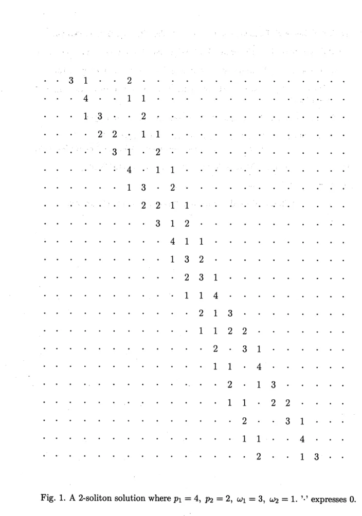
and this expresses the other soliton. The value of thephaseshift of this solution in the case of$L=1$ _{is given} as _follows. $\mathrm{E}\mathrm{q}.(33)$

can

be written

$\rho_{n}^{t}=\max(0,p_{1}n-(p_{1^{-}}1)t-(2p_{2}-1))$, ₍₃₅₎

$= \max(\mathrm{O},p_{1}(n-(2p_{2}-1))-(p_{1}-1)(t-(2p_{2}-1)))$ , (36)

and $\mathrm{E}\mathrm{q}.(34)$ at $t=-\infty$

can

be written

$\rho_{n}^{t}=\max(\mathrm{o},p_{2}n-(p_{2^{-1}})t-(2p_{2}-1))$, ₍₃₇₎

$= \max(\mathrm{O},p_{2}(n-1)-(p_{2^{-1}})(t+1))$. ₍₃₈₎

Therefore the solitons shift their positions

$(2p_{2^{-}}1,2p2-1)$ for the soliton

near

$\eta_{1}\approx 0$,

(39)

$(-1,1)$ _{for the soliton}

near

$\eta_{2}\approx 0$,

in n-t plain. Fig.1 shows the interaction of solitons where we take $p_{1}=4$ and

Similarly, in the

case

of the 2-soliton solution with

$L=1,$ $p_{1}>p_{2}\geq L$,

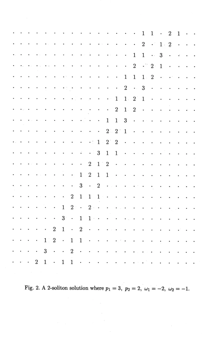
$\sigma_{1}=-1,$ $\sigma_{2}=-1$, (40)

$\eta_{1}^{0}=0,$ $\eta_{2}^{0}=0$,

the phase shift is given by

$(-2p_{2}+1,.2p_{2}-1)$ for

t.he

$\mathrm{S}\mathrm{o}\mathrm{l}\mathrm{i}\mathrm{t}_{0}.\mathrm{n}.$ n

ear

$\eta 1$

-$.\approx.0$,

(41)

$(1, 1)$ for the soliton near $\eta_{2}\approx 0$,

(See Fig.2 where we take $p_{1}=3,p_{2}=2$) and in the case with

$L=1,$ $p_{1}\geq L,$ $p_{2}\geq L$,

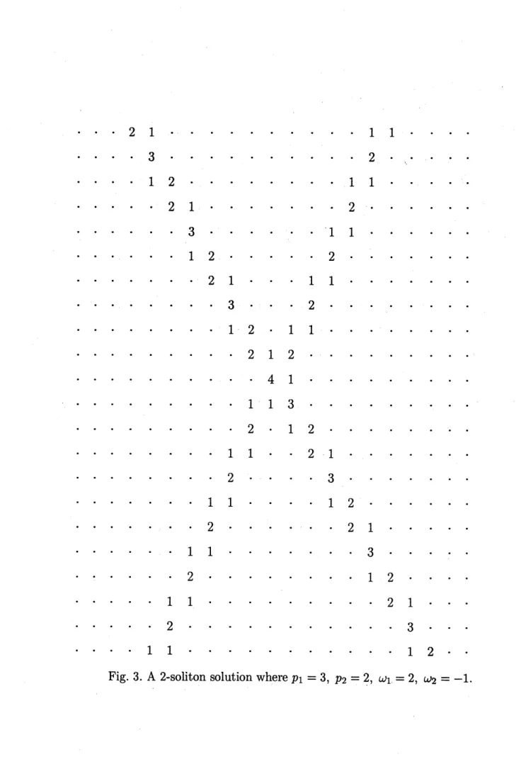
$\sigma_{1}=1,$ $\sigma_{2}=-1$, (42)

$\eta_{1}^{0}=0,$ $\eta_{2}^{0}=0$,

the phase shift is given by

$(1, 1)$ for the soliton near $\eta_{1}\approx 0$,

(43)

$(-1,1)$ for the soliton near $\eta_{2}\approx 0$.

(See Fig.3 where we take $p_{1}=3,p_{2}=2$) These coincide with the result of

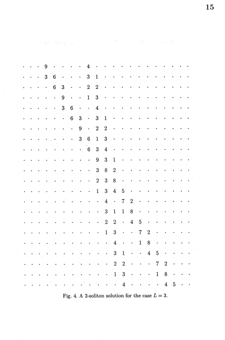
[15]. However in cases other than $L=1$,

a

similar estimate cannot always

be applied because it is possible that the pattern of numbers which soliton

consists of changes after the interaction. See Fig.4 where

we

take $L=3,p_{1}=$

$9,p_{2}=4,$$\sigma 1=1,$$\sigma_{2}=1$.

$\cdot$

Althoughweshowed onlyone- and two-soliton cases, we can also dealwith the interaction of $N$ solitons. For example, the 4-soliton solution shown in Fig.5

in [15] is obtained by setting,

$p_{1}=7$, $p_{2}=3$, $p_{3^{--}}1,$ $p_{4}=-2,$ $L=1$,

$\sigma_{1}=1$, $\sigma_{2}=1$, $\sigma_{3}.=1,$ $\sigma_{4}=-\cdot 1$, (44)

$\eta_{1}^{0_{=-}}10,$ $\eta_{2}^{0}=-1,$ $\eta 30=0,$ $\eta_{4}^{0}=-2$

.

It

can

also be shown that the total phase shift of each soliton of the N-soliton solution is given by the

sum

of phase shifts of each pairwise interaction.

Finally, it should be noted that $\rho_{n}^{t}$ satisfies

$\rho_{nn}^{t+1}+\rho^{t}-1=\max(2\rho n’\rho_{n+\mathrm{i}^{+L}}\beta_{n-}1-ttt)$, (45)

which is obtained from Eqs.(12) and (22), and this

_equation.

ma.y-

be considered

an

analogue of the bilinear identity.

In this paper, we have derived

a

Toda-type CA from the discreteToda lattice equation and given

a

formula for the $N$-soliton solution. This CA inherits the

properties of the Toda lattice equation including solitary

waves

and soliton

interactions. We are currently investigating physical properties, such as con-served $\mathrm{q}\mathrm{u}\mathrm{a}\mathrm{n}\mathrm{t}\mathrm{i}\mathrm{t}\mathrm{i}\mathrm{e}\mathrm{s}[17]$, and physical meaning, in terms of a dynamical system,

and will report our results inforthcoming papers. Also,the algebraic structure of this class of CA’s is to be studied in detail, and $\mathrm{r}\mathrm{e}\mathrm{m}$

. $\mathrm{a}\mathrm{i}\mathrm{n}\mathrm{S}.$

an.

$\mathrm{o}\mathrm{p}\mathrm{e}\mathrm{n}\sim$ question

for the future.

Acknowledgement

The authors would like to thank to Dr. James Keiser for his useful comments and suggestions on this manuscript. And authors $\mathrm{a}\mathrm{I}\mathrm{s}\mathrm{o}\dot{\mathrm{w}}\mathrm{o}\mathrm{u}\mathrm{l}\mathrm{d}$ like to thank to

Ms. Meg Rowland for her editorial assistance. J. Matsukidaira acknowledges the financial support ofRyukoku University.

Appendix

In the

cases

$\sigma_{i}\neq-1$ or $\sigma_{j}\neq-1$, arguments of $\cosh$ in $\mathrm{E}\mathrm{q}.(9)$ do not go to $0$

if

we

take $p_{i}\neq p_{j}$. Therefore when taking $\epsilonarrow+0,$ $\cosh$ terms dominate and

$a_{ij}$ tends to

$a_{ij}= \epsilon\log\frac{\sigma_{i}\sigma_{j}-\cosh((p_{i}+\omega i-p_{j}-\omega_{j})/2\epsilon)}{\sigma_{i}\sigma_{j}-\cosh((p_{i}+\omega i+p_{j}+\omega j)/2\epsilon)}$ ,

$\cdot$.

(A.1)

$\sim\epsilon\log\frac{\exp((p_{i}+\omega i-pj-\omega j)/2\epsilon)+\exp((-p_{i^{-}}\omega i+p_{j}+\omega j)/2\epsilon)}{\exp((pi+\omega i+pj+\omega_{j})/2\epsilon)+\exp((-pi^{-\omega_{i}}-pj-\omega j)/2\epsilon)}.$_’ (A.2)

$\sim\max(\frac{p_{i}+\omega_{i^{-}}pj-\omega j}{2},$ $\frac{-p_{i^{-}}\omega_{i}+pj+\omega j}{2})$

$- \max(\frac{p_{i}+\omega_{i}+pj+\omega_{j}}{2},$$\frac{-p_{i}-\omega_{i}-p_{j}-\omega_{j}}{2})$

,

(A.3)

$\frac{-pi-\omega i+pj+\omega j}{2}-\max(\frac{p_{i}+\omega_{i}+p_{jj}+\omega}{2},$ $\frac{-p_{i^{-}}\omega_{i}-pj-\omega j}{2}))$ ,

(A.4)

$= \max(-\max(p_{j}+\omega_{j}, -p_{i^{-\omega_{i}}}),$$- \max(pi+\omega_{i}, -p_{j}-\omega_{j}))$, (A.5)

$= \max(\min(p_{i}+\omega_{i},..-pj-\omega j.),$ $\min(-p_{i}-\omega_{i},pj+\omega_{j}))$. (A.6)

In the case of $\sigma_{i}=-1$ and $\sigma_{j}=-1$, we need to take special care in the

estimate because the numerator or the denominator of $\mathrm{E}\mathrm{q}.(9)$ goes to $0$.

Let us take $p_{i}>L$ and $p_{j}>L$ as an example. From $\mathrm{E}\mathrm{q}.(8)$, we have

$\frac{\omega_{i}}{2\epsilon}=$ -arcsinh $( \exp(-\frac{L}{2\epsilon})\sinh\frac{p_{i}}{2\epsilon})$ . (A.7)

Considering that the argument of arcsinh diverges and using the asymptotic expansion $\mathrm{a}\mathrm{r}\mathrm{c}\sinh_{X}\sim\log 2x+\frac{1}{4x^{2}}$ for $x\gg \mathrm{O}$, we have

$\frac{\omega_{i}}{2\epsilon}\sim-\log(2\exp(-\frac{L}{2\epsilon})\sinh\frac{p_{i}}{2\epsilon})-\frac{1}{4\exp(-L/\epsilon)\sinh^{2}(p_{i}/2\epsilon)}$ . (A.8)

Therefore

$\frac{p_{i}+\omega_{i}-_{\mathrm{P}jj}-\omega}{2\epsilon}\sim\frac{p_{i}}{2\epsilon}-\log(\sinh\frac{p_{i}}{2\epsilon})-\frac{1}{4\exp(-L/\epsilon)\sinh^{2}(p_{i}/2\epsilon)}$

$- \frac{p_{j}}{2\epsilon}+\log(\sinh\frac{p_{j}}{2\epsilon})+\frac{1}{4\exp(-L/\epsilon)\sinh^{2}(pj/2\epsilon)}..(\mathrm{A}.9)$

Here consider expanding each term in series of exponential functions and

es-timating the asymptotic behavior. The first and

_s.e.cond

terms of the r.h.s. of

Eq.(A.9) become

$f$

$\frac{p_{i}}{2\epsilon}-\log(\sinh\frac{p_{i}}{2\epsilon})=-\log\frac{\exp(p_{i}/2\epsilon)-\exp(-pi/2\epsilon)}{2\exp(p_{i}/2\epsilon)}$,

$=- \log\frac{1-\exp(-pi/\epsilon)}{2}\sim\log 2+\exp(-\frac{p_{i}}{\epsilon})+\frac{1}{2}\exp(-2\frac{p_{i}}{\epsilon})+\cdots$,(A.10)

and the third term becomes

$\frac{1}{4\exp(-L/\epsilon)\sinh^{2}(pi/2\epsilon)}..\sim\frac{1}{\exp(-,\prime L/\epsilon)(\exp(pi/2\epsilon)-\exp(-p_{i}/2\epsilon))2}.$,

Thus we obtain

$\frac{p_{i}+\omega_{i}-p_{j}-\omega j}{2\epsilon}\sim\exp(-\frac{p_{i}}{\epsilon})+\frac{1}{2}\exp(-2\frac{p_{i}}{\epsilon})+\cdots-\exp(-\frac{p_{i}-L}{\epsilon})$

$- \exp(-\frac{p_{j}}{\epsilon})-\frac{1}{2}\exp(-2\frac{p_{j}}{\epsilon})-\cdots+\exp(-\frac{p_{j}-L}{\epsilon})$,

$\sim\exp(-\frac{p_{j}-L}{\epsilon})-\exp(-\frac{p_{i}-L}{\epsilon})$. (A. 12)

Substituting this into the argument of $\cosh$ in the numerator of $\mathrm{E}\mathrm{q}.(9)\mathrm{a}\mathrm{n}\mathrm{d}$

using $\cosh x-1=2\sinh^{2}\frac{x}{2}\sim\frac{x^{2}}{2}$ for $x\ll 1$,

$a_{ij} \sim\epsilon\log\{\frac{1}{2}(\exp(-\frac{p_{j}-L}{\epsilon})-\exp(-\frac{p_{i}-L}{\epsilon}))\}2$

.

$- \epsilon\log\{\cosh\frac{p_{i}+\omega_{i}+pj+\omega_{j}}{2\epsilon}-1\}$, $\sim 2\max(-pj.+L, -.p_{i}+L)-L$,

$=-2 \min(pi,p_{j})+L$, _(A.13)

where

we use

the fact $p_{i}+\omega_{i}+p_{j}+\omega_{j}\sim 2L$.

Similarly considering all other possible cases, we obtain

$a_{ij}=-2 \min(|p_{i}|, |p_{j}|)+L$. (A.14)

References

[1] See for example, Theory and Applications

_of

Cellular $Automata\sim$_’ ed. by S.

Wolfram, (World Scientific, Singapore, 1986).

[2] B. Grammaticos, A. Ramani, and V. Papageorgiou, Phys. Rev. Lett. 67 (1991)

1825.

[3] M.Bruschi, O.Ragnisco, $\mathrm{p}.\mathrm{s}_{\mathrm{a}}\mathrm{n}\mathrm{t}\mathrm{i}\dot{\mathrm{m}}$, and G.Tu. Physica D49 (1991) 273. [4] V.Papageorgiou, F.Nijhoff, H.Capel, Phys. Lett. A 155 (1991) 377.

[5] Y.Ohta, R.Hirota, S.Tsujimoto and T.Imai, J.

_Ph..ys.

$\mathrm{S}_{0}\mathrm{c}\sim$

.

Jpn. 62 (1993) 1872. [6] R. Hirota and S. Tsujimoto, J. Phys. Soc. Jpn. 64 (1995) 3125.

[7] K. Park, K. Steiglitz, and W.P. Thurston, Physica D19 (1986) 423.

[8] T.S. Papatheodorou, M.J. Ablowitz, and Y.G. Saridakis, Stud. in Appl. Math. 79 (1988) 173.

[9] A.S. Fokas, E.F. Papadopoulou, Y.G. Saridakis, Physica D41 (1990) 297.

[10] M.J. Ablowitz, J.M. Keiser and L.A. Takhtajan, Phys. Rev. A 44 (1991) 6909. [11] M. Bruschi, P.M. Santini and O. Ragnisco, Phys. Lett. A 169 (1992) 151. [12] T.Tokihiro, D.Takahashi, $\acute{\mathrm{J}}.\mathrm{M}\mathrm{a}\mathrm{t}\mathrm{S}\mathrm{u}\mathrm{k}\mathrm{i}\mathrm{d}\mathrm{a}\mathrm{i}\mathrm{r}\mathrm{a}$

and J.Satsuma, Phys. Rev. Lett. 76

(1996) 3247.

[13] D. Takahashi and J. Satsuma, J. Phys. Soc. Jpn. 59 (1990) 3514.

[14] See Problem 9 in S. Wolfram, Physica Scripta T9 (1985) 170

or S. Wolfram, Cellular Automata and Complexity(Addison Wesley) Page457.

[15] D. Takahashi and J. Matsukidaira, Phys. Lett. A 209 (1995) 184.

[16] R. Hirota, J. Phys. Soc. Jpn. 43 (1977) 2074.

31 2

. . .

₄

. .

_{1 1}

.

.

. . .

.

.

.

.

$\cdot$ -.: . $\cdot-$

.. .

.

_{1 3}

.

.

2

. . . .

..

.

.

. .-

.

. . . .

.

. . .

2 2

..

1 .1

. . . .

.

.

..

.

. . .

.

. . .

...

.

..

_.

3 1

.

2 $-$

:

.

. . . .

.

. .

.

.

: ₄ .r _{1 1} .

. .

.

.

. . .

. .

.

.

.

. . .

. .

_{1 3}

.

2

.

.

.

.

.

.

.

. .

.-

. .

. .

.

.

.

.

.

2 2 1 1

.

.

.

.

.

.. .

.

. .

. .

.

. . . .

.

3 1 2

. . .

.

.

. . .

. .

. . . . .

.

.

. .

4 1 1

. .

.

.

. .

.

.

.

.

.

.

. . . .

_{1 3 2}

. . . . .

.

.

. .

. . .

.

.

.

.

. .

.

_{2 3 1}

.

.

.

. . .

. .

.

.

.

. .

.

. . .

_{1 1 4}

.

. . . .

. . .

. .

. .

. . .

.

.

.

.

2 1 3

.

.

. . . . .

.

. .

.

.

.

.

. .

.

.

.

1 1 2 2

.

.

. . . .

.

.

.

.

. .

. .

.

.

.

2

.

3 1

. .

.

.

.

.

.

.

. . .

. .

.

.

. .

1 1

.

4

. .

.

.

.

.

.

.

.

.

. .

.

. . .

..

. .

2

.

1 3

. .

. .

. .

.

.

. .

..

.

.

. .

.

.

1 1

.

2 2

.

.

.

. .

. .

.

. . .

. . .

.

.

.

₂

.

.

_{3 1}

.

.

.

. .

.

.

.

.

. . .

. .

.

_{1 1}

. .

₄

.

.

. . . . .

.

. .

.

. . . .

.

.

2

.

.

1 3

.

1 1 2 1

. .

. .

.

.

.

. . .

.

. . . .

₂

.

₁ $\cdot 2$

.

.

.

.

.

. . .

. . .

. . .

1 1

..

3

.

..

. .

$\sim$

.

.

.

.

.

.

. . . . .

2 .-, 2 1

. .

. . . . .

..

. .

.

.

. .

_{1 1 1. 2}

.

.

$\cdot$

.

.

. .

.

.

.

.

.

.

.

.

. .

₂

.

₃

. .

.

.

.

.

.

. .

.

.

_{1 1 2 1}

. . . .

.

...

$\cdot$

. . .

.

.

.

.

.

.

2 1 2

.

.

.

. .

.

.

.

.

.

. . . .

_{1 1 3}

.

. . . . .

.

.

. .

. .

..

.

2 2 $\tau 1$

.

. .

. .

.

.

.

. .

.

.

.

.

.

$\cdot$ 1 2 2

. .

. . .

. .

.

. . .

.

. .

.

.

_{3 1 1}

. . .

.

.

. .

. .

.

_{2 1 2}

. . . . .

.

. .

. . .

$\backslash$ $\cdot$

.

.

.

1 2 1 1

. .

.

. .

.

.

.

. .

.

.

.

.

, ₃

.

₂

.

.

.

_.-

.

. . . .

.

.

. .

.

.

_{2 1 1 1}

.

. .

.

.

. .

.

.

.

. . . .

_{1 2.}

.

₂

.

.

.

.

.

.

.

.

. .

. .

.

.

.

₃

.

_{1 1.}

.

.

.

.

. $\cdot$

. .

.

.

.

.

.

2 1

.

2

. . . . .

.

. .

. .

.

1 2

.

1 1

.

.

.

. . . .

. .

₃

. .

2

.

.

. .

.

. . . .

.

2 1

.

1 1

. .

.

.

. .

.

.

. . . .

2 1 1 I

. .

₃

. .

. . . .

.

2

.

$\tau$

.

.

.

. .

1 2

.

.

.

.

. . .

.

1 1

.

. .

.

.

.

.

₂ 1‘

. . .

.

. .

.

2

. . . . .

.

.

.

.

3

.

.

. .

$\cdot$

.

.

1 1

.

.

. . .

.

.

.

.

1 2

. . .

. .

2

.

. .

. . .

.

.

. . .

2 1

.

. .

1 1

.

.

.

.

.

.

. .

. .

. .

3

. .

.

2

.

. . .

.

.

.

.

. .

. .

.

1. 2

.

1 1

. .

. . . . .

.

. . . .

_{2 1 2}

.

.

.

.

. . . .

. . .

.

. .

. .

_{4 1}

. . . .

.

. . .

. .

.

. . . .

1 1 3

. . . .

.

. . .

.

.

.

.

. .

.

₂

.

1 2

.

. .

.

.

.

.

.

. . . .

.

₁ 1

.

.

2 . ₁

.

.

.

.

.

.

. .

.

. . .

2

.

.

. .

3

.

.

.

. . .

. .

. . .

1 1

.

.

.

.

1 2

. .

.

.

.

.

. . .

.

2

.

.

.

. .

.

2 1

.

.

.

.

.

. .

.

1 1

.

. .

. .

.

.

3

. . .

.

.

.

.

.

2

. .

.

.

. . .

1 2

.

.

.

. . .

_{1 1}

.

. .

.

.

.

. .

_{2 1}

. .

. .

.

₂

. . . .

.

. .

.

. . .

3

.

.

.

.

_{1 1}

. . . .

.

. . .

.

_{1 2}

.

9 4

.

.

.

3 6

. . .

3 1

.

.

.

. . .

.

. .

.

.

.

.

.

_{6 3}

.

.

2 2

.

.

.

.

.

. .

. .

.

. . . .

.

₉

.

.

$\dot{1}$ 3

. .

.

. . . .

.

. .

. .

.

$\cdot$

..

$\cdot$.

.

3 6

. .

4

. . . .

. .

. .

. .

.

. . . . .

6 3

.

3 1

. . . .

. .

.

. .

.

.

. .

.

. . . .

9

.

2 2

. . .

. .

.

4

.

.

. . . . .

.

.

.

_{3 6 1 3}

. . . .

.

.

. . .

. . . .

.

. .

...

_{6 3 4}

. .

. .

. .

.

. .

. .

. .

.

.

.

. .

_{9 3 1}

. .

. . .

.

. .

.

.

. .

.

. . . .

_{3 8 2}

. . .

.

. .

. .

.

.

. .

. .

.

.

.

₂ 3 8

. . .

.

. .

.

.

.

.

.

.

.

. .

.

.

1 3 4 5

. .

.

. .

.

.

.

. .

.

.

.

.

. .

.

4

.

7 2

.

. .

.

. .

.

. .

.

. .

.

_{3 1} 1 8

. .

.

.

.. .

.

.

. . .

. .

.

.

2 . ₂

.

4 5

. .

.

.

.

. . .

.

. . .

.

.

.

_{1 3}

.

.

_{7 2}

. . . .

. . .

.

.

. .

.

. .

..

4

. .

1 8

. . . .

.

.

.

. .

.

.

.

.

.

.

_{3 1}

.

.

_{4 5}

.

.

.

. . .

.

.

. .

. . . .

2 2

. . .

7 2

. .

.

. . . .

.

1 3

. .

.

1 8

. ..

. . .

.

.

.

. . . .

.

.

4

.

. .

.

4 5

.