2007, Vol. 50, No. 4, 463-487
MULTI-PERIOD OPTIMIZATION MODEL FOR A HOUSEHOLD, AND OPTIMAL INSURANCE DESIGN
Norio Hibiki Keio University
(Received October 17, 2006; Revised May 7, 2007)
Abstract We discuss an optimization model to obtain an optimal investment and insurance strategy for a household. In this paper, we extend the studies in Hibiki and Komoribayashi (2006). We introduce the following points, and examine the model with numerical examples.
1
ç We consider cash çow due to a serious disease and involve medical insurance. 2
ç An optimization model is formulated with term life insurance which variable insurance money is received.
3
ç We propose a model to decide optimal life and medical insurance money received at each time. 4
ç Sampling error is examined with 100 kinds of 5,000 sample paths.
Keywords: Finance, multi-period optimization, ånancial planning, investment and in-surance strategy, inin-surance design
1. Introduction
We discuss an optimization model to obtain an optimal investment and insurance strategy for a household. Recently, ånancial institutions have promoted giving a ånancial advice for individual investors. A household is exposed to risk associated with the decrease in real ånancial wealth due to inçation, loss of wage income due to the householder's death, loss of a house or non-ånancial wealth due to the åre, and the increase in medical cost due to a serious disease. Financial institutions need to recommend appropriate ånancial products in order to hedge risk against these accidents. We clarify how a set of asset mix, and life, åre and medical insurance aãect asset and liability management for a household. We develop a multi-period optimization model which involves determining a set of ånancial products, hedging risk associated with a life cycle of a household and saving for the old age. The simulated path approach [3, 4] can be used to solve this problem.
There are some studies in the literature for individual optimal investment strategy; Bodie, Merton and Samuelson [1], Merton [7, 8], Samuelson [10]. Chen, Ibbotson, Milevsky and Zhu [2] advocate an optimization model with the inclusion of wage income, consumption expenditure, and both optimal asset allocation and life insurance. Yoshida, Yamada and Hibiki [12] solve an optimal asset allocation problem for a household using a multi-period optimization approach. Hibiki, Komoribayashi and Toyoda [6] describe a multi-period op-timization model to determine an optimal set of asset mix, life insurance and åre insurance in conjunction with their life cycle and characteristics. The model is examined with numer-ical examples. In addition, some ånancial advices for three households are illustrated for
practical use, and results which coincide with a practical feeling are obtained.
Hibiki and Komoribayashi [5] extend the studies in Hibiki, Komoribayashi and Toyoda [6] for practical use. Risk associated with the householder's death is hedged by life insurance. The model is proposed involving the associated three factors: receipt of a survivor's pension, exemption from mortgage loan payments, and change in the consumption level. Additional eãects by three factors are examined with numerical examples. Moreover, the sensitivity of parameters associated with home buying is analyzed in order to examine the home buying strategy.
We obtain the following practical and interesting results in Hibiki, Komoribayashi and Toyoda [6], and Hibiki and Komoribayashi [5].
(1) The older a householder is, the less optimal life insurance money is.
(2) Optimal åre insurance money is nearly equal to the maximum loss of non-ånancial wealth.
(3) Expected terminal ånancial wealth does not aãect optimal life and åre insurance money.
(4) If a household receives a survivor's pension and keeps the consumption level lower after a householder died, optimal life insurance money and investment units of a risky asset are reduced.
(5) If loan payments are forgiven due to the householder's death, optimal investment units of a risky asset are reduced, but optimal life and åre insurance money are not inçuenced.
(6) Home buying strategy aãects an optimal asset mix and life insurance money. In this paper, we extend the studies in Hibiki and Komoribayashi [5]. We introduce the fol-lowing points in a multi-period optimization model, and examine the model with numerical examples.
1
ç We consider cash çow due to a serious disease and involve medical insurance to cover the expensive medical cost.
2
ç An optimization model is formulated with term life insurance which variable insur-ance money is received, and it is compared with the constant receipt of life insurinsur-ance money by using numerical examples.
3
ç We propose a model to decide optimal life and medical insurance money received at each time.
4
ç Sampling error is examined with 100 kinds of 5,000 sample paths.
This paper is organized as follows. We describe a household, income, consumption expen-diture, and four kinds of ånancial products, or securities, life insurance, åre insurance, and medical insurance to develop a model in Section 2. Section 3 shows the formulation of a multi-period ALM optimization model for a household. We analyze the sensitivity of pa-rameters associated with a serious disease, and examine the eãect of medical insurance. We solve the problem with decreasing life insurance money over time, and compare it with con-stant life insurance money over time by using numerical examples. In Section 4, we propose a model to decide optimal life and medical insurance money at each time, and numerical examples are shown. Sampling error is examined with 100 kinds of 5,000 sample paths in Section 5. Section 6 provides our concluding remarks.
2. Model Structure
We deåne a household, and describe income and consumption expenditure. We clarify the characteristics of ånancial instruments such as securities, life insurance, åre insurance, and
medical insurance. We attach a superscript (i) to a random and path dependent parameter in order to formulate a model in the simulated path approach.
2.1. Household
We deåne a household as a group composed of a householder and members of family as in the previous papers [5, 6]. Wealth at time t held by a household can be divided into two kinds of wealth: ånancial wealth W1;t(i) and non-ånancial wealth W
(i)
2;t. A household is exposed to risk associated with three kinds of accidents: a death and a serious disease of a householder, and a åre of a house. It is assumed that a death of a householder makes wage earnings stop, a serious disease of a householder decreases wage income and makes large payment, and a åre of a house damages a fraction ã of non-ånancial wealth. A householder can purchase a life insurance policy, a åre insurance policy and a medical insurance policy to hedge risk in addition to the investment in securities such as stocks and bonds.
Cash çow streams are inçuenced by risk exposure associated with income and expendi-ture. We set the following parameters associated with the accidents to describe cash çow streams.
ú1;t(i) : one if a householder dies on path i at time t and zero otherwise. ú2;t(i) : one if a åre of a house occurs on path i at time t and zero otherwise. ú3;t(i) : one if a householder is alive on path i at time t and zero otherwise.
ú4;t(i) : one if a householder has a serious disease on path i at time t and zero otherwise.1 ï1;t : mortality rate at time t, or the probability that a person who is alive at time 0
will die at time t, ï1;t = Pr(ú1;t = 1) = 1 I
I
X
i=1
ú1;t(i) where I is the number of simulated paths.
ï2 : rate of a åre (which is assumed to be time independent), or the probability that a åre occurs, ï2 = Pr(ú2;t = 1) = 1 I I X i=1 ú2;t(i).
ï4;t : disease rate at time t, or the probability that a person who is alive at time 0 will have a serious disease at time t, ï4;t = Pr(ú4;t = 1) =
1 I I X i=1 ú4;t(i). 2.2. Income
Income at time t is a householder's wage mtif a householder is alive and investment return from ånancial wealth W1;t(i). If a householder dies, a household cannot get wages, but receive severance pay, and draw a survivor's pension. Amounts of severance pay and a survivor's pension are calculated based on the wage level. Let a(i)tm be the amount of a survivor's
pension. The amount of a survivors' pension is dependent on the time of the householder's death tm. An amount of severance pay e(i)t is also dependent on years of continuous em-ployment(age). When a householder has a serious disease, it is assumed that a fraction ó3 (ó3 < 1) of wage income decreases because a householder has to take a rest from work. Amounts of wage income, severance pay and a survivor's pension, or cash inçow except investment return, borrowing, and insurance money, Mt(i) can be shown as follows :
Mt(i) = ú3;t(i)m (i) t + ê 1 Ä ú3;t(i) ë a(i)tm+ ú (i) 1;te (i) t + 1ft=T gú3;T(i)e (i) T Ä ó3ú4;t(i)m (i) t (t = 1; : : : ; T ) (1) where 1fAg is an indicator function which shows one if the condition A is satisåed, and zero otherwise.
1If ú(i)
2.3. Consumption expenses
There assumes to be two kinds of expenses: living expenses C1;t(i) and payments associated with non-ånancial wealth C2;t(i), such as a house, goods, and repair costs. Besides these costs, we need to pay the restoration cost if a åre of a house occurs.
(1) Expenses for purchasing a house
We assume that a household purchases a house by making a down payment and a debt loan at a bank (Ht). Let te be the time when a house is purchased. The debt loan Hte is
the diãerence between the price of the house and the down payment. The expenditure for the house C2;te is the price of the house, and therefore non-ånancial wealth W2;te increases
by the expenditures C2;te at time te. However, net cash outçow of purchasing the house at
time te is not the price of the house, but the down payment. The household pays the debt loan periodically under the determined mortgage interest rate and the loan period after the time te+ 1. We include periodic payments C1;t2 in the living expense for life (C
(i)
1;t) in this paper.
(2) Restoration cost due to a åre
It is assumed that a fraction ãof non-ånancial wealth W2;tÄ1(i) is damaged and the restora-tion cost A(i)t is paid if a åre of a house occurs. Explicitly,
A(i)t = ú (i)
2;tã(1 Ä çt)W2;tÄ1(i) (2)
where çt is a depreciation ratio of non-ånancial wealth at time t. A(i)t does not aãect non-ånancial wealth.2 Instead, it aãects cash çow streams as shown in Equation (12) in Section 3.2.
(3) Medical cost
It is assumed that a household pays ó2 if a householder has a serious disease such as cancer, cardiac infarction, apoplexy. Payment is ú4;t(i)ó2, and it is included in the living expense C1;t(i).
(4) Living expenses C1;t(i)
The following four kinds of parameters are used to describe living expenses.
C1;t1(i) : cost independent of the householder's death, such as education cost and rent. C2
1;t : annual payment for a mortgage loan (when a householder is alive). ó2 : medical cost due to a serious disease a householder has.
C1;t3(i) : other living expense except C 1(i)
1;t , C1;t2 , and ó2 (when a householder is alive). Next, we explain how to compute the annual payment for the debt loan and other living costs dependent on the householder's death.
1
ç Mortgage loan
If a household purchases a group credit insurance policy, the loan payments are forgiven after a householder died. This shows that an amount of annual payment can be ú3;t(i)C1;t2 . However, the loan payment is not forgiven if a household purchases a house after a house-holder died. By using the condition that ú3;t(i) = 0 for t > te if ú3;t(i)e = 0, the amount of annual
payment for mortgage loan can beê1 Ä ú3;t(i)e + ú
(i) 3;t ë C2 1;t. 2
ç Change of the consumption level
It is assumed that a household can keep a normal consumption level if a householder is alive, however a consumption level must be îtimes a normal level if a householder is dead, 2Non-ånancial wealth decreases by A(i)
t due to a åre, but the same money is spent to recover the loss, and non-ånancial wealth increases by A(i)t .
where î is a parameter associated with a consumption level. For example, we set î = 1 when a household keeps a normal level, and we set î= 0:7 when it has to allow for the 70% consumption level. Therefore, other living cost becomes
n ú3;t(i)+ ê 1 Ä ú3;t(i) ë îoC1;t3(i)= n î+ (1 Ä î)ú3;t(i) o C1;t3(i): (3)
The total living cost is C1;t(i) = C 1(i) 1;t + ê 1 Ä ú3;t(i)e + ú (i) 3;t ë C1;t2 + n î+ (1 Ä î)ú3;t(i) o C1;t3(i)+ ú (i) 4;tó2: (4) 2.4. Securities
Investment in risky assets contributes to a hedge against inçation. We invest in n risky assets and cash. Using a price öjt, a rate of return of a risky asset j at time t is
Rjt = öjt
öj;tÄ1 Ä 1 (j = 1; : : : ; n; t = 1; : : : ; T ): (5) A risk-free rate rt at time t(= 0; 1; : : : ; T Ä 1) is åxed in the period from time t to t + 1. We can assume any probability distributions of Rjt and rt in the simulated path approach if we can sample random paths for Rjt and rt. However, it is assumed that R is normally distributed with the mean vector ñ, and the covariance matrix Ü (R ò N(ñ; Ü)), and rt is constant for all t in this paper. We calculate a price öjt by using Rjt.
2.5. Life insurance
We use term life insurance with maturity T against the householder's death. If a householder purchases a term life insurance policy and dies by time T , a household can receive insurance money. In this model, we look upon life insurance as a ånancial product which can hedge risk associated with wage income earned by a householder.
We assume that a household makes level payment. Because only insured person who is alive pays a premium, a premium of level payment per unit is
yl= †T Ä1X t=0 1 ÄPt k=0ï1;k (1 + g1)t !Ä1 (6) where g1 is a guaranteed interest rate of life insurance with maturity T .
Using the principle of equalization of income and expenditure, insurance money is calcu-lated for the corresponding present value of premium income. We explain how to compute variable life insurance money with various kinds of payment çow at each time.3 Let í
1;t be variable life insurance money per unit of present value of premium income at time t. We have 1 = T X t=1 í1;tï1;t (1 + g1)t = T X t=1 ë1;tí1ï1;t (1 + g1)t (7) where í1;t = ë1;tí1. Equation (7) is transformed, and life insurance money per unit is
í1;t = ë1;t (XT k=1 ë1;kï1;k (1 + g1)k )Ä1 : (8)
3Insurance money of well-known type of life insurance is constant over time, and the problem is solved with constant life insurance in Hibiki, Komoribayashi and Toyoda [6], and Hibiki and Komoribayashi [5].
If ë1;t is constant, life insurance money is constant over time regardless of the time of the householder's death.4
2.6. Fire insurance
A household purchases one year åre insurance to hedge loss of non-ånancial wealth due to a åre. It can update the insurance contract every year, and purchase the åre insurance policy corresponding to the future non-ånancial wealth. Using the principle of equalization of income and expenditure, the relationship between one unit of present value of premium income and the corresponding insurance money í2 is shown as:
1 = í2ï2 1 + g2 ; or í2 = 1 + g2 ï2 (9) where g2 is a guaranteed interest rate of one year åre insurance. It is independent of time t. We can only select a single payment because of one year åre insurance. A premium of single payment per unit yF is equal to a unit of the present value of future premium income (yF = 1).
2.7. Medical insurance
We use term medical insurance with maturity T against a householder's serious disease. If a householder purchases a term medical insurance policy and has a serious disease by time T , it can receive medical insurance money. In this model, we look upon medical insurance as a ånancial product which can hedge loss associated with the expensive medical cost and the decrease in wage income.
We assume that a household makes level payments, and its premium per unit is calculated as5 yb = †T Ä1 X t=0 1 ÄPt k=0ï1;k (1 + g1)t !Ä1 ; (10)
as well as life insurance. The same guaranteed interest rate g1 as life insurance is used. We explain how to compute variable medical insurance money as well as life insurance. Let í4;t be variable medical insurance money per unit of the present value of premium income at time t. We have í4;t = ë4;t (XT k=1 ë4;kï4;k (1 + g1)k )Ä1 : (11)
We deåne the function of medical insurance money with the ë4;t values as well as the ë1;t values for life insurance. If ë4;t is constant, medical insurance money is constant over time.
4We show the following two kinds of functions of life insurance money besides a constant function, which have higher values as a householder dies earlier.
Decreasing linear function : ë1;t= T Ä t + 1 Reciprocal of mortality rate : ë1;t= 1
ï1;t
5A premium of level payment per unit of medical insurance is the same as that of life insurance (Equation (6)) with the same maturity because only insured person who is alive pays a premium. A disease rate inçuences insurance money.
3. Multi-period ALM Optimization Model for a Household
We formulate a multi-period optimization model in the simulated path approach. Condi-tional value at risk (CVaR) is used as a risk measure [9]. We assume that the current time is 0 (t = 0), and a householder retires at time T , which is a planning horizon. As mentioned in Section 2.4, a household invests in n risky assets and cash, and it can rebalance positions at each time. It purchases a T -years life insurance and medical insurance policies at time 0, and makes level payments. It also purchases an one-year åre insurance policy which is updated every year in the planning period.
3.1. Notations (1) Subscript/Superscript j : asset (j = 1; : : : ; n). t : time (t = 1; : : : ; T ). i : path (i = 1; : : : ; I). (2) Parameters6
öj0 : price of risky asset j at time 0 (j = 1; : : : ; n).
ö(i)jt : price of risky asset j on path i at time t (j = 1; : : : ; n; t = 1; : : : ; T ; i = 1; : : : ; I), ö(i)j1 = ê 1 + R(i)j1 ë öj0 (j = 1; : : : ; n; i = 1; : : : ; I); ö(i)jt = ê 1 + R(i)jt ë ö(i)j;tÄ1 (j = 1; : : : ; n; t = 2; : : : ; T ; i = 1; : : : ; I)
where R(i)jt is a rate of return of risky asset j on path i at time t. r0 : interest rate in period 1 or at time 0.
r(i)tÄ1 : interest rate on path i in period t or at time t Ä 1 (t = 2; : : : ; T ; i = 1; : : : ; I). g1 : guaranteed interest rate on life insurance policies.
yl : premium of level payment life insurance per unit, calculated in Equation (6). yL;t(i) : premium of level payment life insurance per unit on path i at time t, calculated
as y(i)L;t= ú3;t(i)yl.
í1;t : life insurance money per unit at time t, calculated in Equation (8).
L(i)t : life insurance money per unit on path i at time t, calculated as L(i)t = ú1;t(i)í1;t. yb : premium of level payment medical insurance per unit, calculated in Equation (10). yB;t(i) : premium of level payment medical insurance per unit on path i at time t,
calcu-lated as yB;t(i) = ú (i) 3;tyb.
í4;t : medical insurance money per unit at time t, calculated in Equation (11). Bt(i) : medical insurance money per unit on path i at time t, calculated as B
(i) t = ú
(i) 4;tí4;t. g2 : guaranteed interest rate on åre insurance policies.
yF : premium of one year åre insurance per unit, set as yF = 1.
í2 : one year åre insurance money per unit, calculated in Equation (9).
Ft(i) : one year åre insurance money per unit on path i at time t, calculated as Ft(i) = ú2;t(i)í2.
ã : loss ratio of non-ånancial wealth due to a åre of a house. çt : depreciation ratio of non-ånancial wealth at time t.
6The other parameters, ú(i)
A(i)t : loss of non-ånancial wealth on path i at time t, calculated in Equation (2). Mt(i) : cash income associated with wage, severance pay, and survivor's pension on path
i at time t, calculated in Equation (1). Ht(i) : debt loan on path i at time t.
Ct(i) : total consumption expenditures on path i at time t, calculated as C (i) t = C (i) 1;t+C (i) 2;t. W1;t(i) : ånancial wealth on path i at time t. W1;0 is an initial ånancial wealth at time 0. W2;t(i) : non-ånancial wealth on path i at time t, calculated as W
(i)
2;t = (1Äçt)W2;tÄ1(i) +C2;t(i). W2;0 is an initial non-ånancial wealth at time 0.
WE : lower bound of expected terminal ånancial wealth. å : probability level used in the CVaR calculation.
Lv;t : lower bound of cash at time t. When Lv;t< 0, the borrowing can be allowed. (3) Decision variables
zjt : investment unit of risky asset j at time t (j = 1; : : : ; n; t = 0; : : : ; T Ä 1). v0 : cash at time 0.
vt(i) : cash on path i at time t (t = 1; : : : ; T Ä 1; i = 1; : : : ; I). uL : number of life insurance bought at time 0.
uF;t : number of one year åre insurance bought at time t (t = 0; : : : ; T Ä 1). uB : number of medical insurance bought at time 0.
Vå : å-VaR used in the CVaR calculation. q(i) : shortfall below å-VaR (V
å) of terminal ånancial wealth(W1;T(i)) on path i, q(i) ë maxêV
åÄ W1;T(i); 0
ë
(i = 1; : : : ; I). 3.2. Formulation
Cash çow constraints are important in a multi-period optimization approach. Cash çow except trading ånancial assets D(i)t is associated with income, expenditures, and insurance. Premium payment is not required at time T . It is formulated as:
Dt(i) = M (i) t + H (i) t Ä C (i) t Ä 1ft6=T g ê y(i)L;tuL+ yFuF;t + y(i)B;tuB ë + L(i)t uL+ Ft(i)uF;tÄ1 +Bt(i)uBÄ A(i)t (t = 1; : : : ; T Ä 1; i = 1; : : : ; I): (12) The objective is the maximization of the CVaR associated with terminal ånancial wealth subject to the minimum return requirement.7 Namely,
CVaRå= Max ( VåÄ 1 (1 Ä å)I I X i=1
q(i)åååååW1;T(i) Ä Vå+ q(i) ï 0 (i = 1; : : : ; I)
)
Expected terminal ånancial wealth E[W1;T] is deåned as a return measure, and therefore the minimum return requirement is formulated as
1 I I X i=1 W1;T(i) ï WE:
7Even if the CVaR of W
0ÄW1;T(i) is used to minimize the objective, we have the same solution as the solution derived from the maximization of the CVaR of W1;T(i).
The model is formulated as follows: Maximize VåÄ 1 (1 Ä å)I I X i=1 q(i); (13) subject to n X j=1 öj0zj0+ v0+ yL;0uL+ yFuF;0+ yB;0uB= W1;0; (14) (W1;1(i) =) n X j=1 ö(i)j1zj0+ (1 + r0)v0+ D1(i) = n X j=1
ö(i)j1zj1+ v(i)1 (i = 1; : : : ; I); (15)
(W1;t(i) =) n X j=1 ö(i)jtzj;tÄ1+ ê
1 + r(i)tÄ1ëvtÄ1(i) + D(i)t = n X j=1 ö(i)jtzjt+ vt(i) (t = 2; : : : ; T Ä 1; i = 1; : : : ; I); (16) W1;T(i) = 8 < : n X j=1 ö(i)jTzj;T Ä1+ ê 1 + r(i)T Ä1ëvT Ä1(i) 9 = ;+ D(i)T (i = 1; : : : ; I); (17) 1 I I X i=1 W1;T(i) ï WE; (18)
W1;T(i) Ä Vå+ q(i) ï 0 (i = 1; : : : ; I); (19) zjt ï 0 (j = 1; : : : ; n; t = 0; : : : ; T Ä 1); v0 ï 0; vt(i) ï Lv;t (t = 1; : : : ; T Ä 1; i = 1; : : : ; I); uLï 0; uF;tï 0 (t = 0; : : : ; T Ä 1); uB ï 0; q(i) ï 0 (i = 1; : : : ; I); Vå : free: 3.3. Numerical analysis 3.3.1. Setting
We test numerical examples using the same setting of the family and the parameters as in Hibiki and Komoribayashi [5]. We show the sensitivity analysis associated with a serious disease because the model involves medical insurance.
All of the problems are solved using NUOPT (Ver. 7.1.5) { mathematical programming software package developed by Mathematical System, Inc. { on Windows XP personal computer which has 2.13 GHz CPU and 2GB memory.
The householder is thirty years old and the spouse is twenty-eight years old. The årst child is an infant aged 0, and the second child will be born in three years.8 The householder works at a ånancial institution, and the household plans that it will prepare twenty million yen as a down payment ten years later and buy an apartment in the center of Tokyo which costs åfty million yen. Twenty million yen is paid at the time (te = 10) when the house is bought. Thirty million yen is borrowed, and the mortgage loan is equally paid over twenty years. Equal yearly payment is calculated at a mortgage investment rate of 6%. The parents make an educational plan that the children will go to a private elementary school, a private 8It is assumed that the second child is not born if the householder dies in two years.
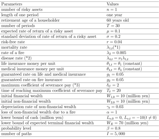
junior high school, a private high school, and a private university. The parameter values used in the examples are shown in Table 1.
Table 1: Parameter values
Parameters Values
number of risky assets n = 1
length of one period one year
retirement age of a householder 60 years old
number of periods T = 30
expected rate of return of a risky asset ñ= 0:1 standard deviation of rate of return of a risky asset õ= 0:2
risk-free rate r = 0:04
mortality rate ï1;t(*1)
rate of a åre ï2 = 0:005
disease rate (*2) ï4;t = ó1ï1;t
life insurance money per unit í1;t = í1 (constant)
medical insurance money per unit í4;t = í4 (constant)
guaranteed rate on life and medical insurance g1 = 0:05
guaranteed rate on åre insurance g2 = 0:05
maximum coeécient of severance pay (*3) éU = 2 time of reaching maximum coeécient of severance pay Té= 20
initial ånancial wealth W1;0 = 10 (million yen)
initial non-ånancial wealth W2;0 = 10 (million yen)
depreciation rate of non-ånancial wealth çt = 0:03 loss of non-ånancial wealth due to a åre ã = 1
lower bound of cash (million yen) Lv;0= 0, Lv;t= Ä10(t 6= 0) lower bound of expected terminal ånancial wealth WE = 70 (million yen)
probability level å= 0:8
number of paths I = 5; 000
*1 The rates are estimated by the life insurance standard life table 1996 for men [11]. *2 There must be a serious disease rate table for medical insurance, and a premium must be calculated by using the table. However, the table is not published outside. In this paper, we assume that the disease rate ï4;t is ó1(> 1) times the mortality
rate ï1;t. The reason is that a serious disease causes death, and the disease rate
becomes higher with age.
*3 An amount of severance pay e(i)t is calculated by multiplying an amount of wage
when a householder retires or dies with the provision coeécient étin Equation (20).
It is assumed that the provision coeécient is a piecewise linear function with an upper bound éU at time Téin Equation (21). Explicitly,
e(i)t = étm(i)t (t = 1; : : : ; T ); (20) ét = min îí t Té ì ; 1 ï éU (t = 1; : : : ; T ; i = 1; : : : ; I; Téî T ): (21) Wage income depends on householder's age and occupation. We calculate wage income of a householder over time based on the Census of wage in 2003 by Ministry of Health, Labor and Welfare [15]. Consumption expenditure depends on wage income, family structure and
school (education) plan. We calculate average consumption expenditures with respect to each number of family and each income level of family based on the national survey of family income and expenditure in 1999 by Statistic Bureau, Ministry of Internal Aãairs and Communications [16]. We calculate average educational expenses based on the survey of household expenditure on education per student in 2001 [13] , the survey of student life by Ministry of Education, Culture, Sports, Science and Technology [14].
We clarify the eãects of four parameters (factors) associated with a serious disease : 1ç a serious disease rate, 2ç medical cost, 3ç the decrease in wage income, 4ç the possibility of death after having a serious disease. We solve åve kinds of problems for each parameter as in Table 2 to examine the sensitivity of four parameters. When one of the parameters is examined, the other parameter values are åxed at `P3' values. We test 17 combinations in total.9
Table 2: Parameters associated with a serious disease
Parameters Notations P1 P2 P3 P4 P5
Coeécient of a disease rate ó1 2.0 2.5 3.0 3.5 4.0
Medical cost ó2 50 100 150 200 250
Decreasing rate of wage income ó3 0.10 0.15 0.20 0.25 0.30
Death probability after a serious disease(*4) ï3 0.3 0.4 0.5 0.6 0.7
*4 A serious disease causes death, and therefore it is assumed that ï3(< 1 : constant) is
the probability that a householder having a serious disease dies after one year. For example, the probability is 60% if we set ï3 = 0:6.
3.3.2. Result CVaR 38.6 38.8 39.0 39.2 39.4 39.6 39.8 P1 P2 P3 P4 P5 Parameter CV aR (m il li on y en) ν1 ν2 ν3 λ3
Life insurance money
102.2 102.3 102.4 102.5 102.6 102.7 102.8 102.9 P1 P2 P3 P4 P5 Parameter In su ra n ce m on ey (m ill io n y en) ν1 ν2 ν3 λ3 ó1 ó2 ó3 ï3 ó1 ó2 ó3 ï3
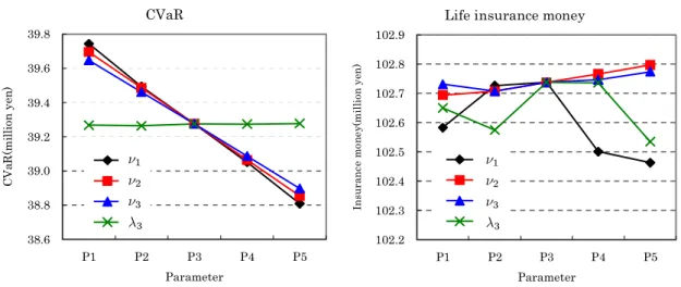
Figure 1: CVaR and optimal life insurance money
Figure 1 shows the CVaR on the left-hand side and life insurance money (í1uÉL) on the right-hand side for each combination of parameters. For example, a broken line of ó1 shows
9For example, when we examine the sensitivity of ó
1 value, we solve the problems with one of åve kinds of ó1 and `P3' values of ó2, ó3 and ï3 (i.e. ó2 = 150, ó3 = 0:20 and ï3 = 0:5). Four combinations are overlapped, and therefore 17(= 5 Ç 4 Ä 3) combinations are tested.
values of the CVaR for åve kinds of ó1, i.e. P1= 2:0 through P5= 4:0 in Table 2.10 When a ó1 value becomes larger, the CVaR value is smaller because the probabilities of the decrease in wage income and the increase in medical cost are higher due to a serious disease. When ó2 and ó3 values become larger, wage income decreases and medical cost increases, and therefore the CVaR value is smaller. However, the CVaR value is not inçuenced by the ï3 value, or the probability of the householder's death after a householder has a serious disease. Life insurance money is not aãected by four factors associated with a serious disease.
Medical insurance money
2.0 2.5 3.0 3.5 4.0 4.5 5.0 P1 P2 P3 P4 P5 Parameter In su ra nc e m one y( m il li on ye n) ν1 ν2 ν3 λ3
Premium of level payment
15 20 25 30 35 40 P1 P2 P3 P4 P5 Parameter P re m iu m ( tho u san d y en) ν1 ν2 ν3 λ3 Units of medical insurance
20 25 30 35 40 45 50 55 60 P1 P2 P3 P4 P5 Parameter un it s ν1 ν2 ν3 λ3 ó1 ó2 ó3 ï3 ó1 ó2 ó3 ï3 ó1 ó2 ó3 ï3
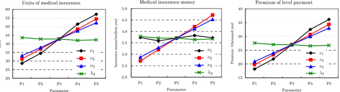
Figure 2: Optimal units, insurance money, and premium for medical insurance Figure 2 shows units of medical insurance (uÉ
B) on the left-hand side, medical insurance money (í4uÉB) on the middle, and premium payments (ybuÉB) on the right-hand side. When ó2 and ó3 values become larger, the householder purchases more units of medical insurance policy to hedge against the decrease in wage income and the amount of medical cost. It means that the number of units of medical insurance and premium payments become larger. Medical insurance money is not inçuenced by the increase in a disease rate ó1 because wage income does not decrease and medical cost does not increase. However, medical insurance money per unit (í4) becomes small, and the householder needs to purchase more units of medical insurance policy(uÉ
B) in order to receive medical insurance money which can cover cash outçow due to a serious disease. Therefore, premium payments (ybuÉB) become large. A ï3 value does not inçuence the number of units of medical insurance, medical insurance money, and premium payments as well as the CVaR and life insurance money.
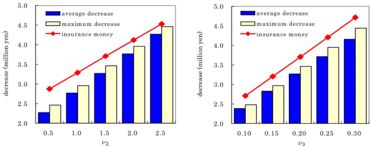
When a householder has a serious disease at time t, ånancial wealth decreases by payment for the expensive medical cost and the decrease in wage income at time t. We examine the relationship between the annual average or maximum decrease in wealth during thirty years and optimal medical insurance money in Figure 3. The decrease in wealth consists of the decrease in wage income and the increase in medical cost. The average and maximum decreases are almost equal to medical insurance money. It shows that medical insurance money is used to hedge against the decrease in cash inçow.
Figure 4 shows optimal investment units of a risky asset for each parameter. Investment units decrease gradually over time. When ó1, ó2, and ó3 values become large, investment units increase. The reason is that a household needs to invest in more amounts of a risky asset to cover the decrease in wage income and the increase in medical cost, and to increase expected terminal wealth. A ï3 value does not inçuence optimal investment units.
10When we show values of the CVaR for åve kinds of ó
1, we can write åve ó1 instead of the expression of P1 through P5 on the vertical axis so that readers understand the meaning of graphs easily. However, we employ the expression as in Figure 1 for lack of space. Readers can know parameter values of P1 through P5 by checking Table 2.
2.0 2.5 3.0 3.5 4.0 4.5 5.0 0.10 0.15 0.20 0.25 0.30 ν3 de cre as e ( m il li on ye n ) average decrease maximum decrease insurance money 2.0 2.5 3.0 3.5 4.0 4.5 5.0 0.5 1.0 1.5 2.0 2.5 ν2 de cre as e ( m il li on y en ) average decrease maximum decrease insurance money ó2 ó3
Figure 3: Relationship between the decrease in wealth and optimal medical insurance money
ν1 5 0 1 0 0 1 5 0 2 0 0 2 5 0 0 5 1 0 1 5 2 0 2 5 3 0 t im e In ve st m ent un it s o f a r isk y as se t ν 1 = 2 .0 ν 1 = 2 .5 ν 1 = 3 .0 ν 1 = 3 .5 ν 1 = 4 .0 ν2 5 0 1 0 0 1 5 0 2 0 0 2 5 0 0 5 1 0 1 5 2 0 2 5 3 0 t im e In ve st m en t u n it s o f a ri sk y as se t ν 2 = 0 .5 ν 2 = 1 .0 ν 2 = 1 .5 ν 2 = 2 .0 ν 2 = 2 .5 ν3 5 0 1 0 0 1 5 0 2 0 0 2 5 0 0 5 1 0 1 5 2 0 2 5 3 0 t im e In ve st m en t u ni ts o f a r isk y as se t ν 3 = 0 .1 0ν 3 = 0 .1 5 ν 3 = 0 .2 0 ν 3 = 0 .2 5 ν 3 = 0 .3 0 λ 3 5 0 1 0 0 1 5 0 2 0 0 2 5 0 0 5 1 0 1 5 2 0 2 5 3 0 tim e In ve st m en t u n it s o f a ri sk y ass et λ 3 = 0 .3λ 3 = 0 .4 λ 3 = 0 .5 λ 3 = 0 .6 λ 3 = 0 .7 ó2 ó1 ó3 ï3 ó2= 0 :5 ó2= 1 :0 ó2= 1 :5 ó2= 2 :0 ó2= 2 :5 ó1= 2 : 0 ó1= 2 : 5 ó1= 3 : 0 ó1= 3 : 5 ó1= 4 : 0 ó3= 0 : 1 0 ó3= 0 : 1 5 ó3= 0 : 2 0 ó3= 0 : 2 5 ó3= 0 : 3 0 ï3= 0 : 3 ï3= 0 : 4 ï3= 0 : 5 ï3= 0 : 6 ï3= 0 : 7
Figure 4: Optimal investment units of a risky asset 3.4. Life insurance with a decreasing linear function
Term life insurance of receiving constant insurance money is a very popular product. We solve the problem to examine the characteristics of the product. Four cases are the combi-nations of two kinds of pf and two kinds of np introduced in Hibiki and Komoribayashi [5], i.e. pf = 0 and np = 0, pf = 0 and np = 1, pf = 1 and np = 0, pf = 1 and np = 1. pf is one if the problem is solved with receipt of a survivor's pension and zero without receipt, and np is one if the problem is solved with exemption from a mortgage loan and zero without exemption.
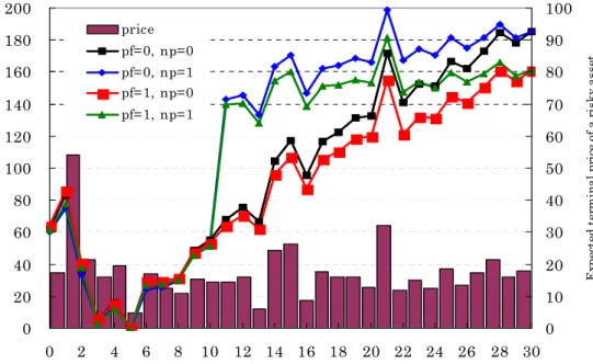
Figure 5 shows conditional expected terminal ånancial wealth at the time of the house-holder's death.11 A value at time 0 shows an expected value under the condition that a householder does not die in the planning period. Expected terminal ånancial wealth is increasing as the time of the householder's death becomes late.12 The reason is that a house-hold gets a wage in the longer period before a househouse-holder dies, and receives life insurance money when a householder dies. If a householder dies earlier, expected terminal ånancial wealth tends to be lower because a household receives a lower survivor's pension relative to an amount of wage. 0 20 40 60 80 100 120 140 160 180 200 0 2 4 6 8 10 12 14 16 18 20 22 24 26 28 30 tim e of the householder's death (0: a householder does not die.)
E xp ec te d te rm in al f in an cia l w ea lt h ( m ill io n y en ) 0 10 20 30 40 50 60 70 80 90 100 Ex pe ct ed t er m in al p ri ce o f a r is ky as se t price pf=0, np=0 pf=0, np=1 pf=1, np=0 pf=1, np=1
Figure 5: Conditional expected terminal ånancial wealth at each time
It is important for a household not to have a ånancial problem and to lead a stable life by receiving life insurance money even if a householder dies earlier. Therefore, we should design life insurance that a household can receive more insurance money as a householder dies earlier. We solve the problem with a decreasing life insurance policy that insurance money decreases in proportion to a householder's age. We calculate í1;t with ë1;t = T Ät + 1 in Equation (8). We solve the problem, and compare a decreasing type of life insurance with a constant type.
11Conditional expected terminal ånancial wealth at each time Wú1
t in Figure 5 can be calculated as follows: Wú1 0 = 1 jú3;Tj I X i=1 ú3;T(i)WT(i); Wú1 t = 1 jú1;tj I X i=1 ú1;t(i)WT(i)(t = 1; : : : ; T ) where jú1;tj = I X i=1 ú1;t(i), and jú3;Tj = I X i=1 ú3;T .
12If a householder dies after time 12, the loan payment is forgiven. Therefore, expected terminal ånancial wealth after time 12 for np = 1 are larger than those for np = 0 because the reduction in loan payment contributes to the increase in terminal ånancial wealth. Broken lines are not smooth, especially at time 1, 14, 15, and 21. The reason is that terminal ånancial wealth (WT(i)) is inçuenced by a terminal price of a risky asset (ö(i)jT).
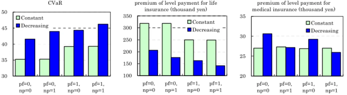
CVaR 30 35 40 45 50 pf=0, np=0 pf=0,np=1 pf=1,np=0 pf=1,np=1 Constant Decreasing
premium of level payment for life insurance (thousand yen)
100 150 200 250 300 350 pf=0, np=0 pf=0,np=1 pf=1,np=0 pf=1,np=1 Constant Decreasing
premium of level payment for medical insurance (thousand yen)
20 25 30 35 pf=0, np=0 pf=0,np=1 pf=1,np=0 pf=1,np=1 Constant Decreasing
Figure 6: CVaR and premium payments for life insurance and medical insurance Figure 6 shows the CVaR values, and premium payments for life insurance and medical insurance. The CVaR values of the decreasing type increases about 7 million yen or 18%, compared with the constant type for pf = 1 and np = 1. Premiums of the decreasing type decreases about 35% for np = 0, and about 45% for np = 1, compared with the constant type. We obtain dramatic eãects by introducing the decreasing type of life insurance. The change in design of life insurance does not inçuence medical insurance money.
pf=0 0 50 100 150 200 250 0 2 4 6 8 10 12 14 16 18 20 22 24 26 28 30 time lif e i n su ra n ce m on ey ( m illion ye n) np=0(Decreasing) np=1(Decreasing) np=0(Constant) np=1(Constant) pf=1 0 50 100 150 200 250 0 2 4 6 8 10 12 14 16 18 20 22 24 26 28 30 time lif e in su ran ce m on ey ( m illi on y en ) np=0(Decreasing) np=1(Decreasing) np=0(Constant) np=1(Constant)
Figure 7: Optimal life insurance money
Figure 7 shows life insurance money at each time without receiving a survivor's pension (pf = 0) on the left-hand side, and with receiving (pf = 1) on the right-hand side. Life insurance money without receiving a survivor's pension is larger than insurance money with receiving for both types. Life insurance money of the decreasing type is larger until time 10, but smaller after 10 than that of the constant type. The reason premiums of constant type are larger than those of the decreasing type is that a mortality rate becomes higher as a householder gets older, and the period more life insurance money can be received for the constant type is longer than the period for the decreasing type.
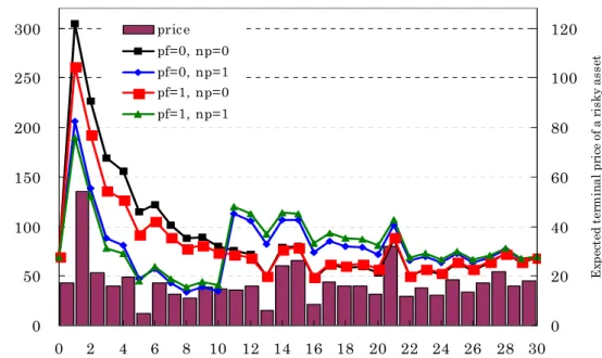
Figure 8 shows conditional expected terminal ånancial wealth at each time of the house-holder's death. When a householder dies earlier, conditional expected terminal wealth becomes larger because a household can receive larger life insurance money.13 Expected terminal ånancial wealth entirely becomes çatter than those in Figure 5. A decreasing type of life insurance reduces risk, and has similar expected terminal ånancial wealth regardless of the time of the householder's death, while a household saves premium payments.
13We might set up a decreasing linear function with higher life insurance money when a householder dies earlier.
0 50 100 150 200 250 300 0 2 4 6 8 10 12 14 16 18 20 22 24 26 28 30 tim e of the householder's death (0: a householder does not die.)
E xp ec te d te rm in al f in an cia l w ea lt h ( m illio n y en ) 0 20 40 60 80 100 120 Ex pe ct ed t er m in al p ri ce o f a r is ky as se t price pf=0, np=0 pf=0, np=1 pf=1, np=0 pf=1, np=1
Figure 8: Conditional expected terminal ånancial wealth at each time 4. Optimal Insurance Design
The results derived in Section 3.4 show that we had better design life insurance so that a household can receive insurance money to åt cash çow needs. We propose a model to decide optimal life and medical insurance money received at each time, instead of the constant or decreasing insurance money.
4.1. Modiåcation for optimal design (1) Life insurance
Life insurance money at time t (xt) is calculated by multiplying life insurance money per unit (í1;t) by the number of units (uL), i.e. xt = í1;tuL. Life insurance money per unit is not given as input parameters, and therefore we need to add a constraint which shows the principle of equalization of income and expenditure instead of Equation (7). We multiply the number of units of life insurance (uL) by both sides in Equation (7), and we obtain
uL = T X t=1 ûtxt where ût= ï1;t (1 + g1)t: (22)
L(i)t uL in Equation (12) is transformed as
L(i)t uL= ú1;t(i)í1;tuL= ú1;t(i)xt (t = 1; : : : ; T ; i = 1; : : : ; I): (2) Medical insurance
Medical insurance money at time t (wt) is calculated as wt = í4;tuB. The principle of equalization of income and expenditure is
uB = T X t=1 †twt where †t= ï4;t (1 + g1)t: (23)
Bt(i)uB in Equation (12) is transformed as
(3) Other constraints
In addition to the modiåcation of the principle of equalization of income and expenditure, we need to add and modify the constraints in the formulation.
1
ç Cash çow except trading assets (Dt(i)) : modiåcation of Equation (12) D(i)t = Mt(i)+ Ht(i)Ä Ct(i)Ä 1ft6=T g
ê
yL;t(i)uL+ yFuF;t+ yB;t(i)uB
ë
+ ú1;t(i)xt+ ú2;t(i)í2uF;tÄ1 +ú4;t(i)wtÄ ú2;t(i)ã(1 Ä çt)W2;tÄ1(i) (t = 1; : : : ; T ; i = 1; : : : ; I): (24) 2
ç Additional non-negativity constraints
xt ï 0 (t = 1; : : : ; T ); (25)
wtï 0 (t = 1; : : : ; T ): (26)
Except for the above-mentioned constraints, we do not have to change the formulation in Section 3.2.
4.2. Numerical analysis
We compare the combination (a) of a decreasing linear function for life insurance and a constant function for medical insurance titled `Decreasing LI'(Life Insurance) with the com-bination (b) of optimal functions for life and medical insurance titled `optimal' in Table 3. We solve the problems for four cases generated by the combination of pf and np.
Table 3: Combination of functions for life and medical insurance life insurance money medical insurance money (a) Decreasing LI decreasing function (í1;tuL) constant function (í4uB) (b) optimal optimal function (xt) optimal function (wt)
CVaR 40 42 44 46 48 pf=0, np=0 pf=0, np=1 pf=1, np=0 pf=1, np=1 Decreasing LI Optimal
premium of level payment for life insurance (thousand yen)
100 120 140 160 180 200 220 pf=0, np=0 pf=0, np=1 pf=1, np=0 pf=1, np=1 Decreasing LI Optimal
premium of level payment for medical insurance (thousand yen)
20 25 30 35 pf=0, np=0 pf=0, np=1 pf=1, np=0 pf=1, np=1 Decreasing LI Optimal
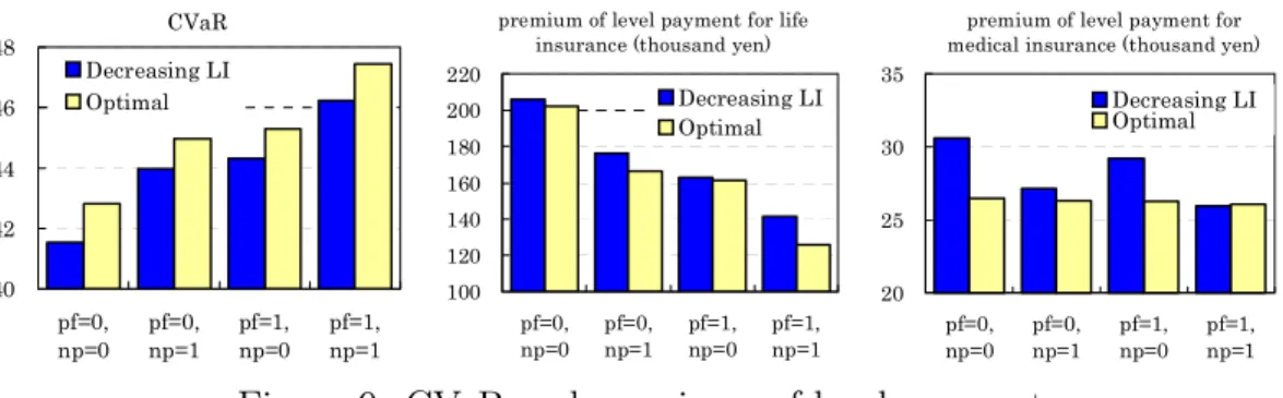
Figure 9: CVaR and premiums of level payment
Figure 9 shows the CVaR values on the left-hand side, premium payments for life insur-ance on the middle, and premium payments for medical insurinsur-ance on the right-hand side. The CVaR values with optimal functions are larger than the CVaR values with a decreasing linear function for life insurance by 1.2 million yen or about 3% for pf = 1 and np = 1. Premium payments for life insurance with optimal functions can be reduced by about 10%. Premium payments for medical insurance can be reduced by 13% for pf = 0 and np = 0, and 10% for pf = 1 and np = 0.
We show optimal functions for life insurance in Figure 10, and describe the characteristics as follow.
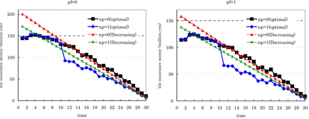
pf=0 0 50 100 150 200 0 2 4 6 8 10 12 14 16 18 20 22 24 26 28 30 time li fe in su ra n ce m on ey ( m il li on y en ) np=0(optimal) np=1(optimal) np=0(Decreasing) np=1(Decreasing) pf=1 0 50 100 150 0 2 4 6 8 10 12 14 16 18 20 22 24 26 28 30 time li fe in su ra n ce m on ey ( m il li on y en ) np=0(optimal) np=1(optimal) np=0(Decreasing) np=1(Decreasing)
Figure 10: Optimal life insurance money 1
ç The optimal functions also become decreasing functions entirely as we expect and examine the eãect in Section 3.4.
2
ç Amounts of optimal life insurance money rise sharply from time 2 to 3. The reason is that the second child will be born at time 3, and it costs for the household to raise the second child (e.g. educational cost14) if the householder dies after time 3. 3
ç Optimal life insurance money drops sharply from time 10 to time 11 for np = 1. The reason is that a house is bought at time 10, and loan payments are forgiven if a householder dies after time 11.15
When we solve the problem with a decreasing type of life insurance, the CVaR value be-comes much larger, and premium payments become much lower drastically, compared with a constant type of life insurance. On the other hand, when we solve the problem with an optimal function of life insurance, the CVaR value becomes larger by 3%, and premium payments become lower by 10%, compared with a decreasing type of life insurance. The eãect using the optimal function is not dramatic. The reason is that the decreasing linear function is similar to the optimal function as shown in Figure 10.
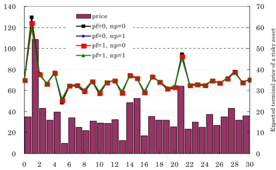
Figure 11 shows conditional expected terminal ånancial wealth at each time of the house-holder's death. They are çatter than those in Figure 8. This shows that conditional expected terminal ånancial wealth at each time has similar values, regardless of the time of the house-holder's death.16 They have almost the same values, regardless of the values of pf and np. The reason is that optimal life insurance money can be adjusted, depending on the values of pf and np as shown from the results in Figure 10. The model involving the optimal insurance design is solved usefully so that the above-mentioned feature can be reçected, and terminal ånancial wealth can get less aãected by the time of the householder's death.
Figure 12 shows medical insurance money on the left-hand side, and åre insurance money on the right-hand side. The broken line with the legend `decrease' on the left-hand side shows the decrease in wealth due to a serious disease, i.e. the decrease in wage income and the amount of medical cost. The broken line with the legend `loss' on the right-hand side shows 14The increases in life insurance money from time 2 to 3 are about 6.7 million yen for pf = 0, and about 8.8 million yen for pf = 1. The value at time 3 of the educational cost is about 8.95 million yen with 4% discount rate.
15The decrease in life insurance money from time 10 to 11 is about 36.4 million yen for np = 1. Annual payment is 2.616 million yen for a mortgage loan of 30 million yen with 6% mortgage interest rate, and therefore the value at time 11 of the mortgage loan payment is 36.97 million yen with 4% discount rate. 16The reason the values at time 1 and 21 are higher is that average prices of a risky asset are higher, and there exists sampling errors.
the loss due to a åre. The left-hand side of Figure 12 shows the same results on average that a medical insurance policy is purchased to cover the decrease in wage income and the amount of medical cost in Section 3.3. However, the amounts of medical insurance money at each time are unstable, and the optimal function of medical insurance is easily aãected by sampling error. Optimal åre insurance money is nearly equal to the maximum loss of non-ånancial wealth as well as the results derived by the previous models.
0 20 40 60 80 100 120 140 0 2 4 6 8 10 12 14 16 18 20 22 24 26 28 30 tim e of the householder's death (0: a householder does not die.)
E xp ect ed t er m in al fi n an ci al w ea lt h (mi lli on y en) 0 10 20 30 40 50 60 70 Ex pe ct ed t er m in al p ri ce o f a r is ky as se t price pf=0, np=0 pf=0, np=1 pf=1, np=0 pf=1, np=1
Figure 11: Conditional expected terminal ånancial wealth at each time
medical insurance money (million yen)
0 1 2 3 4 5 6 7 8 0 2 4 6 8 10 12 14 16 18 20 22 24 26 28 30 time pf=0, np=0 pf=0, np=1 pf=1, np=0 pf=1, np=1 decrease
fire insurance money (million yen)
0 10 20 30 40 50 60 70 0 2 4 6 8 10 12 14 16 18 20 22 24 26 28 30 time pf=0, np=0 pf=0, np=1 pf=1, np=0 pf=1, np=1 loss
Figure 12: Optimal medical and åre insurance money
5. Examining sampling error
We ånd the characteristics of the model with numerical examples. However, sampling error occurs because a thirty-periods model is solved with 5,000 simulated paths. We solve 100 kinds of problems with diãerent random seeds, and we examine sample distributions of optimal solutions. We need to provide 100 kinds of dataset associated with prices of a risky asset (ö(i)j;t), 0-1 parameters for the householder's death (ú
(i) 1;t, ú
(i)
of a åre (ú2;t(i)), and 0-1 parameter for the householder's serious disease (ú (i)
4;t). We call the model with constant life insurance money in Section 3.2 `model A', and the model with optimal life insurance money in Section 4 `model B'.
5.1. Numerical Analysis : Model A
Figure 13 shows the change in the average of the CVaR on the left-hand side, life insurance money on the middle, and medical insurance money on the right-hand side as we increase the problems solved with diãerent random seeds. There are åve kinds of percentiles derived with diãerent random seeds in Figure 13. The average values converge between forty percentile and sixty percentile by solving about thirty problems with diãerent random seeds.
CVaR (million yen)
39.27 39.28 39.29 39.30 39.31 39.32 39.33 39.34 39.35 39.36 39.37 0 20 40 60 80 100
number of random seeds
average 30%
40% 50%
60% 70%
Life insurance money (million yen)
102.6 102.8 103.0 103.2 103.4 103.6 103.8 104.0 104.2 104.4 0 20 40 60 80 100
number of random seeds
average 30%
40% 50%
60% 70%
Medical insurance money (million yen)
3.35 3.40 3.45 3.50 3.55 3.60 3.65 3.70 3.75 0 20 40 60 80 100
number of random seeds
average 30%
40% 50%
60% 70%
Figure 13: Convergence of the CVaR and life and medical insurance money for model A 100 random seeds 100 125 150 175 200 225 250 275 0 5 10 15 20 25 30 time in ve st m en t u n it s Percentile 100 125 150 175 200 225 250 275 0 5 10 15 20 25 30 time in ve st m en t u n its 0% 25% 50% 75% 100%
Figure 14: Optimal investment units of a risky asset
We show the number of investment units of a risky asset for 100 kinds of random seeds on the left-hand side, and for åve kinds of percentiles on the right-hand side in Figure 14. We ånd that the number of investment units of a risky asset decreases through time as in Figure 4.
Percentiles change smoothly through time because percentiles are calculated separately at each time. The values over time are volatile as in Figure 4 when each problem is solved. However, the values are expected to çuctuate around the average values over time. Let zkÉ 1t be the optimal number of investment units for a risky asset when the problem is solved with the k-th random seed. The average of zkÉ
1t at time t for 100 kinds of problems is as zÉ1t = 1 100 100 X k=1 z1tkÉ(t = 0; : : : ; T Ä 1):
Let DkÉ
z be the average of deviation from the average zÉ1t for each random seed as DkÉz = 1 T T Ä1X t=0 ê z1tkÉÄ zÉ1t ë (k = 1; : : : ; 100): A standard deviation of DkÉ
z is 1.69, a maximum value is 4.35, and a minimum value is Ä3:72. These values are much smaller than the number of investment units, and therefore it can be said that the values zkÉ
1t çuctuate around the average zÉ1t.
We show conditional expected terminal ånancial wealth at each time of the householder's death for 100 kinds of random seeds on the left-hand side, and for seven kinds of percentiles on the right-hand side in Figure 15. We ånd the same characteristics as in Figure 5 even if we use diãerent random seeds.
100 random seeds -20 0 20 40 60 80 100 120 140 160 180 200 0 5 10 15 20 25 30
Time of the householder's death (0: a householder does not die.)
E xp ecte d te rm inal fi na nc ia l w ea lt h (m illio n y en) Percentile -20 0 20 40 60 80 100 120 140 160 180 200 0 5 10 15 20 25 30
Time of the householder's death (0: a householder does not die.)
E xp ec te d te rm ina l f in anc ia l w ea lt h (m illio n y en) 0% 25% 50% 75% 90% 95% 100%
Figure 15: Conditional expected terminal ånancial wealth at each time for model A 5.2. Numerical analysis : Model B
We show life insurance money for 100 kinds of random seeds on the left-hand side, and for åve kinds of percentiles on the right-hand side of Figure 16. We obtain optimal solutions stably even if we use diãerent random seeds. The amounts of life insurance money rise until time 3, and decline afterward.
We show medical insurance money for 100 kinds of random seeds on the left-hand side, and for åve kinds of percentile on the right-hand side of Figure 17. The åfty percentile (median) on the right-hand side of Figure 17 is almost equal to the sum of the decrease in wage income and the amount of medical cost, and therefore we ånd a medical insurance policy is purchased to cover the loss due to a serious disease. However, the amounts of optimal medical insurance money çuctuate around the average as shown on the left-hand side of Figure 17, and we cannot ignore the inçuence of sampling error.
We show conditional expected terminal ånancial wealth at each time of the householder's death for 100 kinds of random seeds on the left-hand side, and for seven kinds of percentiles on the right-hand side of Figure 18. We can ånd the characteristics shown in Figure 11 that terminal ånancial wealth can get less aãected by the time of the householder's death. The åfty percentile (median) on the right-hand side of Figure 18 is almost çat. Some values
100 random seeds 0 20 40 60 80 100 120 140 0 5 10 15 20 25 30 time L if e i n su ra n ce m one y ( m il li on ye n) Percentile 0 20 40 60 80 100 120 140 0 5 10 15 20 25 30 time L if e ins u ra nc e m oney ( m il li on y en) 0% 25% 50% 75% 100%
Figure 16: Optimal life insurance money for model B
100 random seeds 0 1 2 3 4 5 6 7 8 9 0 5 10 15 20 25 30 time M edi ca l in su ra n ce m on ey ( m illi on ye n ) Percentile 0 1 2 3 4 5 6 7 8 9 0 5 10 15 20 25 30 time M edic al i n su ra nc e mo n ey (mill io n ye n ) 0% 25% 50% 75% 100% decrease
Figure 17: Optimal medical insurance money for model B
100 random seeds 40 60 80 100 120 140 160 0 5 10 15 20 25 30
Time of the householder's death (0: a householder does not die.)
Expe ct ed t er m in al f ina nc ia l w ealt h (m illi on ye n ) Percentile 40 60 80 100 120 140 160 0 5 10 15 20 25 30
Time of the householder's death (0: a householder does not die.)
Ex pe ct ed t erm in al fin an cia l we al th ( m il li on y en ) 0% 25% 50% 75% 90% 95% 100%
çuctuate widely in the earlier periods because the number of paths that the householder dies is few,17 and they are aãected by prices of a risky asset. Figure 19 shows conditional expected terminal prices at each time of the householder's death. The çuctuation is due to sampling error because prices are not aãected by the householder's death. Figure 19 is very similar to Figure 18. If we have enough paths at each time of the householder's death, and conditional prices become stable (çat) over time, time series of conditional wealth become also çat. 100 random seeds 0 10 20 30 40 50 60 70 80 0 5 10 15 20 25 30
Time of the householder's death (0: a householder does not die.)
T er m in al pric e Percentile 0 10 20 30 40 50 60 70 80 0 5 10 15 20 25 30
Time of the householder's death (0: a householder does not die.)
Te rm in al p ric e 0% 25% 50% 75% 90% 95% 100%
Figure 19: Conditional expected terminal prices at each time of the householder's death
6. Concluding Remarks
In this paper, we extend the optimization model for a household in Hibiki and Komorib-ayashi [5], and examine the models with numerical examples.
A household is exposed to risk associated with payments for the high cost due to the householder's disease in addition to the decrease in cash inçow due to the householder's death, and the decrease in non-ånancial wealth due to a åre. We consider the associated cash çow, and we propose the model involving medical insurance to hedge risk against payments for the high cost of medical care. We describe cash çow streams in consideration of four parameters and analyze the sensitivity of these parameters : 1ç coeécient of a disease rate, 2ç medical cost, 3ç decreasing rate of wage income, and 4ç death probability after a serious disease. When a disease rate and medical cost are higher, and the decrease in wage income is larger, respectively, the CVaR is lower, the number of medical insurance is larger, and a premium payment is higher. However, the death probability after a disease does not aãect these values. Medical cost and the decrease in wage income are the increasing factors of medical insurance money. Even if a disease rate becomes higher, premium payments become higher, but medical insurance money does not increase. Optimal medical insurance money is almost equal to the sum of the decrease in wage income and the amount of medical cost, and therefore it can be said that a medical insurance policy is purchased to cover the loss due to a serious disease.
The number of units of life insurance with the constant receipt is a decision variable in Hibiki, Komoribayashi and Toyoda [6], and Hibiki and Komoribayashi [5] because the amount of life insurance money is almost constant in practice. Expected terminal ånancial wealth becomes lower when a householder dies earlier, while it becomes higher than neces-sary when a householder dies later. As a result, a household has to pay relatively a high premium. It is important for a household not to have a ånancial problem and to lead a sta-ble life by receiving life insurance money even if a householder dies earlier. We examine the eãect of life insurance that a household can receive more insurance money as a householder dies earlier. By purchasing a decreasing type of life insurance, while premium payments are dramatically reduced, a household can receive large conditional terminal ånancial wealth on average even when a householder dies early, compared with purchasing the constant type.
We had better design life insurance that a household receives life insurance money so that it can åt cash çow needs, and therefore we propose a model to decide optimal life and medical insurance money at each time, instead of constant or decreasing insurance money. We can determine optimal time-dependent life insurance money to tailor cash çow needs of a household, and we ånd it is an useful model that expected terminal ånancial wealth are not inçuenced by the time of the householder's death.
We examine the model with numerical examples to ånd the characteristics. Sampling error occurs because a thirty-periods model is solved with 5,000 paths. We provide 100 kinds of dataset with diãerent random seeds, and solve the problems. We obtain a sample distribution of optimal solutions. Sampling error occurs, but the average value and the values between 25 percentile and 75 percentile clearly show the feature of the optimal solutions.
The extended model can describe a detail cash çow of a household, compared with the previous models. It derives the optimal insurance and investment strategies appropriately, and we can use the model for giving a ånancial advice to individual investors.
References
[1] Z. Bodie, R.C. Merton and W. Samuelson : Labor supply çexibility and portfolio choice in a life-cycle model, Journal of Economic Dynamics and Control, 16 (1992), 427{449. [2] P. Chen, R.G. Ibbotson, M. Milevsky and X. Zhu : Human capital, asset allocation,
and life insurance, Financial Analysts Journal, 62-1 (2006), 97{109.
[3] N. Hibiki : Multi-period stochastic programming models for dynamic asset allocation, Proceedings of the 31st ISCIE International Symposium on Stochastic Systems Theory and Its Applications, 37{42.
[4] N. Hibiki : Multi-period stochastic programming models using simulated paths for strategic asset allocation, Journal of Operations Research Society of Japan, 44-2 (2001), 169{193 (in Japanese).
[5] N. Hibiki and K. Komoribayashi : Dynamic ånancial planning for a household in a multi-period optimization approach, Journal of the Japanese Association of Risk, Insurance and Pensions, 2-1 (2006), 3{31(in Japanese), and The tenth annual APRIA(Asia-Paciåc Risk and Insurance Association) Conference, 2006.
[6] N. Hibiki, K. Komoribayashi and N. Toyoda : Multi-period ALM optimization model for a household, Journal of the Japanese Association of Risk, Insurance and Pensions, 1-1 (2005), 45-68 (in Japanese). The paper reported in IFORS 2005(Honolulu) can be downloaded from
[7] R.C. Merton : Lifetime portfolio selection under uncertainty: the continuous-time case, Review of Economics and Statistics, 51-3 (1969), 247{257.
[8] R.C. Merton : Optimum consumption and portfolio rules in a continuous-time model, Journal of Economic Theory, 3-4 (1971), 373{413.
[9] R.T. Rockafellar and S. Uryasev : Optimization of conditional value-at-risk, Journal of Risk, 2-3 (2000), 21{41.
[10] P.A. Samuelson : Lifetime portfolio selection by dynamic stochastic programming, Review of Economics and Statistics, 51-3 (1969), 239{246.
[11] The Institute of Actuaries of Japan : Life insurance standard life table (1996).
[12] Y. Yoshida, Y. Yamada and N. Hibiki : Multi-period optimization model for household asset allocation problem, Department of Administration Engineering, Keio University, Technical report, No.02-003, 2002 (in Japanese).
[13] Ministry of Education, Culture, Sports, Science and Technoloty : The survey of house-hold expenditure on education per student in 2002, 2003,
http://www.mext.go.jp/b menu/toukei/001/006/03121101.htm .
[14] Ministry of Education, Culture, Sports, Science and Technology : The survey of student life in 2002, 2003, http://www.mext.go.jp/b menu/houdou/16/04/04040702.htm . [15] Ministry of Health, Labour and Welfare : Wage income of the household over time
based on the Census of wage in 2003, 2003,
http://wwwdbtk.mhlw.go.jp/toukei/kouhyo/indexk-roudou.html .
[16] Statistic Bureau, Ministry of Internal Aãairs and Communications : The national survey of family income and expenditure(1999), 2000,
http://www.stat.go.jp/data/zensho/1999/021index.htm.
Norio Hibiki
Department of Administration Engineering Faculty of Science and Technology
Keio University
3-14-1 Hiyoshi, Kohoku-ku, Yokohama 223-8522, Japan E-mail : hibiki@ae.keio.ac.jp