A Quarterly Econometric Forecasting Model for Taiwan Economy

(1)

Southeast Asian Studies,Vol. 17, No.2, September 1979

A

~uarterly

EconolDetric Forecasting

Model for Tai-wan EconoD1.Y

Vi-Chung CHIU*

I Introduction

This is a revised quarterly model1) of DGBAS: Directorate-General of Budg-et, Accounting & Statistics [1]. The main purpose of this model is the short-term forecast for the Taiwan economy. Because the short-run fluctuations are

mainly caused by demand and price

factors, the major parts of the model is built by equations related to these factors. To reflect the characteristics of the Taiwan economy, the model takes into account the following facts: first, the Taiwan economy is export-oriented [2]; i.e., the private investment is mainly

stimulated by exports;2) second, the in-creasing openness of the economy [3],

I.e., the impact from outside are

increasingly strong;3) third, the potential GNP will be enlarged by the accom-plishment of the Ten Major Projects.4 )

In regard to the forecast, one difficult problem is how to consider the shock caused by the severance of the diplomatic relationship between the Republic of China and the United States. So far, however, no serious problem seems to have been posed by this palitical factor.

II The Model

A Structure of the Model

The model consists of 28 behavioristic and institutional equations and 24

... Council for Economic Planning & Develop-ment, Executive Yuan, Taipei, Taiwan

I) The modified equations are private fixed investment, inventory investment, export, import, labor demand, wage rate, wholesale price index, consumer price index, price de-flator of inventory investment, price dede-flator of export, demand for money, total deprecia-tion and depreciation in private sector function. It should be pointed out that the Aggregate and Supply Model designed by

280

definitions. There are 52 endogenous variables and 19 exogenous variables.

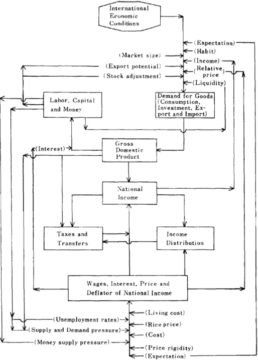
The structure of the model 1S

represented by the flow chart as follows:

Professor T. C. Liu in 1967 [4] laid the basis of present model. Had it not been for Prof. Liu, the present model could not have been completed.

2) Please see the equation of private fixed investment in section II.

3) Please see the equation of wholesale price index in section II.

(2)

Y. e. eHlU: A Quarterly Econometric Forecasting Model for Taiwan Economy

International Economic Conditions

0('-(Expecta ti on) ( :-'larket size) ~~(Habit) (Export potentia]) ----Jl

IE-(Income) - - ,

I' ~CRela.tive) __T""'1

(Stock adjustment) ~ price

~CLiquidity)

~ Demand for Goods

'" fE-- Labor, Capi taI ( Consumption.

and Money Investment.

Ex--

port and Import)

~

CInterest)4 Gross_Domestic Product

:\ational

...

Income

11\

\ It I,

Taxes and , Income

Transfers Distribution

Wages, Interest. Price and Deflator of National Income

,

---.. (Unemploymentrates)~

~CLivingcost) F -(Rice price)

'----L.(Supply and Demand pressure)-7

~(Cost)

II _{CMoney supply pressure) --;;.}

!'E--CPrice rigidity) ~(Expectation) Fig. 1 The Flow Chart of the Model

B List of Variables (Subscript "$"

refers to "current price") 1. Endogenous Variables

( I) C_f Private food consump-tion ( 3) IpTiv : (4-) ] (5) X (6) M sumption

Private fixed investment

Inventory investment Export of goods and serVIces

Import of goods and Private nonfood con- serVIces

(3)

property and enterprises (27) TgJ$: Transfer payments from

government to households

(28) TJg$: Transfer payments from

households to government

(29) GJ$ Private food

consump-tion

serVIces

Grossfixed investment by government

Inventory investment

Export of goods and

Import of goods and

servIces

Total depreciation

Gross domestic product (at current prices)

Gross domestic product (at 1971 constant prices) National income

Disposable income Total demand Total supply Property income

Price deflator of total supply (or total demand) Price deflator of gross domestic product

Price deflator of private (40) Gdp (37) M$ (35)

J$

(36) X$ (38) D$ (39) Gdp$: (41) NI$ : (42) Yd$ : (43) TD$: (44) TS : (45) Prop$: (46) P (47) POdP : (48) Pc consumption (49) M.$: Money supply

(50) K Total capital stock

(51) K priv : Private capital stock (52) KJ Inventory stock 2. Exogenous Variables

( 1)

G

g$ Government consumption

( 2) 1pc$ Gross fixed investment by

public enterprises

( 3) 1'1$ Gross fixed investment by government

( 4) Rg$ : Interest on public debts

( 5) FIa$: Net factor Income from

abroad

( 6)

Taf$:

Transfer payments from

abroad to family ( 7) Pr Rice price index Indirect taxes

Business direct taxes Direct taxes

Public enterprise savings Government income from Labor demand

Wage rate

Wholesale price index Consumer price index Price deflator of food consumption

Price deflator of nonfood consumption

Price deflator of govern-ment consumption

Price deflator of fixed investment

Price deflator of

inven-Private nonfood

con-sumption

Government consumption Private fixed investment Gross fixed investment by public enterprises (7) NL ( 8)

W

(9) WP1: (10) GPI (11) PCI (13) Peg

(12)

Pco (22) T,$ : (23) TF$: (24) T(!.$ (25) Se$ (26) Yg$ (31) Gg

(32) Ipo

d,,$ : (33) Ipc tory investment

(16) P:Jt: Price deflator of exports

(17) Ma Demand for money

(18) Wage$: Wage income

(19) A$ Mixed income (20) D Total depreciation (21) Dpr,v: Depreciation In private sector 282 - - - -

(4)

~---Y. C. emu: A Quarterly Econometric Forecasting Model for Taiwan Economy

1970 IV

(16) DUMu : Dummy variable,

DUM_{74 :} I,after 1974I; 0, before 1973 IV _ 0034 Pc, (0.018) PGtlP/IOO +0.741 C'-l (0.088) +0.545 DUM74+1.798 Ql (0.326) (0.149) -0.653 Q2+ 0 .492 Q3 (0.258) (0.160) R2=0.991 82=0.175 d=2.549

( 2) Private N01ifood Consumption Yd$ Co=27.043+0.186 PII00 (0.042) -0226 Pc!> (0:034) Pc/100 +0.148

p1.'to

(0.026) +3.923 Ql+0.185 Q2 (0.305) (0.339) +2.420 Q3 (0.325) R2=0.991 82=0.697 d=2.136

( 3 ) Private Fixed Investment

IprffJ= 1.050 +0.146

t

(C,+CO)-i i=1 (0.023) 4 +0.028

:LX-

i i=1 (0.015) -0.049 Kpri"-l (0.013) -2.894 Ql-2.118 Q2 (0.485) (0.477) -0.757 Q3 (0.477) R2=0.903 82₌ _1.931 d=1.983 ( 4 ) Inventory Investment J=0.582-0.309 X-O.095 Kj -1 (0.110) (0.041) +0.318 Gdp_1-5.192 Ql (0.116) (1.097) -1.365 Q2- 4.631 Q3 . (0.879) (0.879) Dummy variable, Ql: 1, for 1st quarter; 0, otherwise Dummy variable, Q2: 1, for 2nd quarter; 0, otherwise Dummy variable, Q3: 1, for 3rd quarter; 0, otherwise (19) Q3 (18) Q2

Price deflator of imports Imports price index (in US$)

Effective exchange rates W orId export price index

World trade quantum

index

(13) 1. Interest rate

(14) u Unemployment rate

(15) DUMn : Dummy variable,

D UM_{n :} I, after 1971 I; 0, before (10) e (II) PW : (12) TW: (8) Pm (9) P{..

C Esthnated Structural Equations and Identities

The structural equations are estimated by OLS using the time series from 1st quarter of 1962 to the 4th quarter of 1978. The figures in the parentheses under the coefficients of the equation are the standard errors.

1. Estimated Structural Equations ( I) Private Food Consumption

Yd$

C.r=4.504+0.062 P /100 (0.020) Gap

(5)

R2=0.410 S2=6.527 d= 1.155

( 5) Export of Goods and Services X=-15.320+0.062 TW

(0.051 )

+0106 PW (0:083) e1100· WPII100 +0.656 X-I +0.017 K_1 (0.106) (0.013) -1.909 QI

+

1.960 Q2 (1.037) (1.081) +0.823 Q3 (1.047) R2=0.980 S2=8.577 d=2.181

( 6) Import of Goods and Services M=8.121 +0.440 Gdp (0.064) +0.298 X-I (0.086) -0211 -

P:"~~

(0:066) elI 00· WPIfl OO -1.605 QI+1.609 Q2 (0.836) (0.838) +0.448 Q3 (0.853) R2=0.979 S2=5.657

d=

1.374 ( 7 ) Labor Demand NL=2.544 +0.012 Gdp+O.029 Gdp-l (0.007) (0.007) -0261 _ W (0:126) PGdP/lOO -0.059 QI- 0 .017 Q2 (0.064) (0.048) +0.133 Q3 (0.057)

R2=0.984

82

_=0.013

d=0.599 ( 8) Wage Rate W=20.123 -2.714 u+O.532 CPI (0.909) (0.075) 284 +0.202 Gdt -0.898 Ql (0.201) NL _(2.095) -1. 708 Q2-1.131 Q3 (2.118) (2.099)

R2=0.648

8

2

_=30.194

d=0.817

( 9 ) Wholesale Price Index WPI=75.500+0.338 Pm (0.117) +0.032 DUMn-Pm (0.030) +0.163 DUMu ·P71I (0.040) + 15.027

N,£.

(8.307) Gdp -2.719

~d'Pl

+0.491

Ql (1.892) (2.100) +0.411 Q2+ 0 .459 Qa (2.064) (2.198) R2=0.981 S2=32.614 d=0.559 (l0) Consumer Price Index

CPI=-0.965 +0.351 WPI+3.417 W (0.032) (0.881) +0.578 CPL1-0.749 Ql (0.044) (0.861) +0.167 Qz+ 1.250 Q3 (0.859) (0.858) R2=0.997 S2=6.233 d= 1.425

( 11 ) Price Deflator

rif

Food Consumption

Per=-14.738 +0.044 Pr+ 1.025 CPI (0.017) (0.079) +0.092 P_{er -}l -0.055 Ql (0.065) (0.960) +0.579 Q2+ 1.390 Qa (0.948) (0.938) RZ=O.998 82_=7.356 d-0.927

(12). Price Deflator

rif

Norifood

(6)

Y. C. emu: A Quarterly Econometric Forecasting~Iodelfor Taiwan Economy Pco =8.203+0.454 CPI (0.066) +0.463 p ..u -1+ 1.512 Ql (0.082) (0.730) -0.028 Q2-0.278 Q3 (0.742) (0.729) RZ=0.997 S2==4.517 d=0.621

(13) Price Diflator qf Government Con-sumption Pcg= -22.042+0.674 P (0.109) +0.490 pc,,-1-·0.713 Ql (0.086) (2.113) +1.075 Q2+3.219 Q3 (2.127) (2.114) R2=0.990 S2==37.573 d=2.548

(14) Price Diflator

cif

Fixed Investment Pi= 10.957 +0.326 P m+3.410 ~V (0.094) (1.491) +0.501 Pi - 1+2.769 Ql (0.121) (1.792) +2.363 Qz+2.500 Q3 (1. 796) (1. 787) R2=0.986 SZ=26.973 d= 1.285

(15) Price Diflator of Inventory Investment

Pj =3.956+0.158 Pm (0.123) +0.796 WPI+4.031 Q1 (0.154) (2.713) +2.242 Q2+ 3.656 Q3 (2.703) (2.692) R2=0.963 S2=61.431 d=I.845

(16) Price Diflator

cif

Export P:c=-4.155 +1.018 WPI-0.480 Q1 (0.024) (2.598) -0.638 Qz+O.225 Q3 (2.598) (2.597) R2=0.966 SZ=57.325 d=0.816 (17) Demandfor Money In Md= -0.027 +0.891' (0.135) In (Ct+Co+C,,+Ipriv +Ipc+Ig

+

J)+0.253· (0.058) In X-O.363 In i+O.l03 Ql (0.096) (0.025) +0.042 Q2+0.092 Q3 (0.027) (0.030) R2=0.988 S2=0.005 d=0.488 (18) Wage Income Wage$=5.002 +2.216 (Wx NL ) (0.035) -1.115 Q1 +0.517 Q2 (1.282) (1.283) -0.878 Q3 (1.281) R2=0.984 S2= 13.950 d=0.383 (19) j\1.ixed Income A$=2.902 +0.149 (WageS +Prop$) (0.006) -0.514 Ql-2.696 Q2 (0.660) (0.660) -1.443 Q3 (0.659) R2=0.905 S2=3.685 d= 1.593 (20) Total Depreciation D= -5.272+0.012 K_1_+K (0.0002) 2 +29.199

~dP

+0.012 Q1 (3.090) -1 (0.100) +0.160 Q2+ 0 .049 Q3 (0.100) (0.103) R2=0.985 S2=0.081 d. 0.54.7 .

(21) .Depreciation hi Private Sector

(7)

D prio =-3.951 +0.007 K priv +Kprtv -1 (0.001)

2

+20.543 Gdp (2.535)

K

priv -1 -0.301 QI-0.327 Q2 (0.136) (0.136) +0.188 Qa (0.139) R2=0.900 82=0.152 d=

1.657

(22) Indirect Taxes T,$=-1.003 +0.159 Gdp$-0.494 Ql (0.002) (0.306) +0.524 Q2-0.027 Qa (0.306) (0.305) R2=0.993 82_=0.791 d=2.701 (23) Business Direct Taxes

Tp$=-1.412 +0.124 (NI$+Rg$-Yg$ (0.007) -A$-Wage$)+0.312 Ql (0.231) +0.967 Q2+ 1.507 Qa (0.231) (0.230) R2=0.848 S2=0.451 d=1.706 (24) Direct Taxes Td$=-2.355 +0.071 (NI$ +Rg$

(0.002)

- Yg$) +1.021 Ql (0.229) + 1.550 Q2+ 1.627 Qa (0.229) (0.229) W=O.963 82_=0.446 d=1.574

(25) Public Enterprise Savings

8e$=-0.061 +0.022 Gdp$ -0.219 Ql .(0.001) .. (0.128) +0.063 Q2- 0 .005 Qa (0.127) (0.127) RZ=0.989 8z=0.137 d=I.770

(26) Government Income from Property and Enterprises Yg$=0.376 +0.029 Gdp$ +0.057 Ql (0.003) (0.525) + 1.682 Q2- 0.501 Qa

(0.524)

R2=0.639 82=2.331 d=2.044

(27) Transfer Payments from Govern-ment to Households Tg,$=-0.065 +0.003 Gdp$ +0.063 Ql (0.0002) (0.050) +0.154 Qz-O.045 Qa (0.050) (0.050) W=0.722 82_=0.022 d-1.803

(28) Transfer Payments from House-holds to Government T,g$ = -0.509 +0.034 NI$+0.019 Ql (0.002) (0.247) +0.294 Qz-0.407 Qa (0.246) (0.246) RZ=0.847 8z=0.514 d=1.713

2. Identities

(29) G,$ =G,'Pc , /100 (30) Go$=Go·Pco/l00 (31)

G

g= P

Gil

oo

cg (32) Iprav$=Iprtv'Pdl00 (33) I Ipc$ pe= Pi/100 (34)

(8)

I(J=ph(Jl~O.-Y. C. CHIU: A Quarterly Econometric Forecasting l'vIodelforTaiwan Economy (35) J$=J·P j /l00 (44) TS=Cdp+AI (36) X$=X·Pz/I00 (45) Prop$=NI$+R g$- TF$-Sc$ (37) M$=M·Pm/l00 - Yg$- WageS-AS (38) D$=D·Pijl00 (46) P TD$ X 100 (39) Cdp$=C1$ +Co$ +Cg$+IpTiv$ TS +Ipc$+Ig$+J$+X$-M$ (47) POdP= CdP$Cdp X 100 (40) Cdp=C I+Co

+C

g+IpTiv +1pc CI$+Co$+C~~ X 100 +Ig+J+X-M (48) Pc _Ct+Co+C_g (41 ) NI $=Cdp$ - Ti$ -D$ +Fla$ (49) M,$ =i"Ud·P/ 100

(42) Yd$=NI$- Td$- Yg$-Sc$ (50) K -K_₁=Ipriv +Ipc+Ig-D

+ T gI$- T jg $+ Tat$+R g$ (51 ) K pTiv -Kpriv-l =IpTiv -DpTiv

(43) TD$=Cdp$+M$ (52) Kj-Kj-1=J

III Discussion of the Equations

Private Food Consumption The explanatory

variables in food consumption function are disposable income, relative price of food, and food consumption lagged by one period [5]. There is a dummy variable (DUM_u 1 after 1974 I ;=0 before 1973 IV) in food consumption function to reflect an upward-shift of that function after 1974, when the world-wide recession occurred.S)

According to the estimated food con-sumption function, the short-run and long-run MPC of food were 0.062, 0.239 respectively during the sample period. The price elasticity was 0.173 in the 4th quarter, last year.6 ) The upward-shift of consumption function after 1974 was

5) As food consumption maintain the ordinary increasing rate in the recession period after 1974, so food consumption function will shift upwards.

6) Elasticity of private food consumption with respect to price

= ~- X

.1:.-

c=0.034 x 5.093==0.173

or Cf

-0.545 billion NT$ at 1971 price7 ) (0.031 billion US$ at current prices).

Private Nonfood Consumption Disposable

income and a relative price are related to nonfood consumption function. There is another explanatory variable, real liquidity, in this function to serve as an approximation of wealth effect.

MPC of nonfood was 0.186 during the sample period. The price elasticity was 0.608 in the 4th quarter last year.8 ) The nonfood consumption would increase by 0.148 billion NT$ if liquidity increased by 1 billion NT$.9)

Private Fixed Investment The major factors that determine private fixed investment

7) Please see the coefficient of DUM74 of food

consumption function.

8) Elasticity of private nonfood consumption with respect to price

ac

p

= -dPD.- X ---t'-- =0.226X2.692=0.608

o

9) Please see tht> coefficient of

P1t'~O

of nonfood consumption function.

(9)

17~ 2~}

- X

are expected export, expressed by sum-4

mation of lagged exports (L X-i), ex-i=1

13) The portion caused by intended inventory investment

= 116.436 xO.318=37.027 (billionNT$) 14) The portion caused by unintended inventory

investment

= 73.039X0.309= 22.569 (billion NT$) Major Projects.

In the 4th quarter last year, the elasticity of export with respect to the world trade and competitive power was ventory stock depends on expectation of sales, expressed by gross domestic product lagged by one period; realized sales, expressed by export; and stock adjust-ment, expressed by inventory stock lagged by one period. I t may be interpreted that the change in inventory stock caused by expectation of sales is intended, and the one caused by realized sales is unintended [7]. According to the esti-mated results of the total change in inventory stock, 2.324 billion NT$, in the 4th quarter of 78, the portion caused by intended inventory investment was 37.027 billion NT$,13) the portion caused by unintended inventory investment was -22.569 billion NT$,14) the residual:

-12.716 billion NT$ was caused by

stock adjustment, seasonal change and other factors.

Exports The explanatory variables are

the world trade, competitive power

(

e/lOO'~I/IOO),

capital stock lagged by one period and export lagged by one period.

K_₁ is a proxy for production capacity. I t is used to express the impact of the construction of infrastructure in the Ten

-

al

priv X

- 4

oL: X_i

i=l =0.415

II) Elasticity of private fixed investment with respect to the expected sales of consumer's goods

10) Elasticity of private fixed investment with respect to expected export

4

L:

X_i i=l =0.028X 14.825 I priv _.--_OI-"l'riv 4

o

L:

(C/+CO)_i t=1 =0.146x 12.869 = 1.879

12) The elasticity of private fixed investment with respect to capital stock

=

aa!

priv X Kpriv-1 =0.049x 28.993 Kpriv-l lpriv

,-" 1.421

pected sales of consumers' goods In domestic market, expressed by summation

• 4

of lagged consumptIOn

(t:

(CJ+Co)-t), t=1

and stock adjustment, expressed by capital stock lagged by one period (Kpriv-l)

[6]. All these factors are included In private fixed investment function as explanatory variables, and the estimated results are significant.

The expected exports IS included,

because it is believed that the expectation of sales expansion at foreign markets makes domestic enterprises increase their investment.

In 1978 IV, the elasticities of investment wi th respect to the expected sales of export goods the same of consumers' goods and capital stocks are 0.415,10) 1.87911 ) and

1.42112 ) respectively.

Inventory Investment The change in

(10)

Y. C. CHIU: A Quarterly Econometric Forecasting l\lodelforTaiwan Economy 0.131 and0.220respectively.IS) The same

with respect to production capacity and X-I are 0.202% and 0.640o~ respective-ly.16) Imports M depend on Gdp, X-I, and relative price

(elIOO.

~~11TOO).

The inclusion of Gdp as an explanatory variable is based on the consideration that import increases as production ex-pands, because Taiwan is poor in natural resources.

X-I is then the proxy for import capability or source of foreign exchange for imports [8J. In the sample period, marginal propensity to import was 0.440.

Labor Demand Demand for labor depends

on expected production, expressed by domestic production lagged by one period, and real wage rate. The realized employment is, however, adjusted

Sl-nlultaneously with the actual production (Gdp).

~Vage Rate The change of wage rate is determined by the gap between labor

15) The elasticity of exports with respect to the world trade

ax TW ,

aTW- x

-x--

=0.062x2.114=0.131 The elasticity of export with respect to com-petitive power

-

(j~fmp~ xCo;p--= 0.1 06 x 2.077= 0.220

h C PW

were amp: e.

wpj-16) The elasticity of export with respect to production capacity

()~~-;

X

!5X~

= 0.017X 11.892= 0.202 The elasticity of export with respect to market

Size

c= -

()~~-

X X.:

t

=0.656><0.976=0.640

supply and demand; i.e., unemployment rate [9J, the changes of produc6vity and living costs.

f;Vholesale and Consumer Prices Wholesale price (WP1) depends on import price, excess money supply

(-%d~-)

[I OJ, and demand-supply pressure

(~dP

y7)

There are dummy variables in the coefficient of import price to express the increasing important effect of import price on Taiwan economy due to the increasing openness of the economy.l8)

Consumer price depends on wholesale

prices and wage rate. The rigidity of the price is expressed by consumer pnce lagged by one period. Rigidity is taken into account similarly In the following

price functions.

The Implicit Price D~flator The implicit price deflators are largely determined by wholesale price (WP1) and consumer price (CPI) . The price of rice is used as an explanatory and policy variable in the deflator of food consumption function. I t is virtually controlled by government.

Demand for Money Demand for money

is determined by interest rate and the quantity of goods sold in domestic and foreign markets. The elasticity of demand for money with respect to the total transaction and the interest rate are

17) Capital stock is the proxy for potential productivity, and gross domestic is the expenditure for final products.

18) According to the wholesale price function, the coefficients ofPm are 0.338

during-1961-1971, 0.370 during 1971-1974, 0.533 during 1974-1978.

(11)

1.144 and 0.363 respectively.19)

Wage Income Wage income is determined

by the wage rate and employment. The portion of the payments other than wages such as fringe benefits was 2% according to the estimation of this function.

Mixed Income Mixed income that comes

from agricultural and unincorporated enterprise sectors is explained by wages plus porperty income (Wage$+Prop$) [11] .

Other Equations Depreciation is

deter-mined by capital stock and adjusted by

17~ 2~'

production level. Tax is determined by taxable income. According to the es-timation, the average tax rates were 15.9% for indirect tax, 7.1 % for direct tax, and 12.4% for profit tax. Transfer payments from government to households such as pension, public assistance and scholarship are explained by production level (GdP$). Transfer payments from

households to government such as

donation, administration and penalty fees are explained by national income.

IV Test of the Model

The test in this section is the final-test suggested by Prof. Goldberger [12].

The test statistics for the sample period is that of Theil U inequality coefficient

[13].

where

P: Computed value A: Actual value.

According to the historical simulation result (1965 1-1978 IV), the model performs quite well. The Theil U co-efficients are 2.6% for domestic pro-duction (Gdp), and 1.7% for general price (P).

V Concluding RelDarks

According to the forecasting ex-periences by DGBAS [14], the results are quite satisfactory.20) But more attention

19) The elasticity of demand for nlOney with respect to total transaction

olnMd

=0.891 +0.253=1.144

The e1ast~city of demand for money with respect to interest

alnMd

&TrlT = 0.363

290

should be given to the adjustment of the investment and export functions. Due to the severance of the diplomatic relationship between the Republic of China and the United States, the

fune-20) According to the forecast for the fourth quarter, 1978 by DGBAS, gross domestic product is 124.371 billion NT$ at 1971 prices, wholesale price index is 195.04, while actual values of these two variables are 124.316 billion NT$ and 191.45. The errors are 0.04%, 1.88% respectively.

(12)

Y. C. CHIU: A Quarterly Econometric Forecasting Model for Taiwan Economy tions of these two equations will be

disturbed and should be adjusted. Nev-ertheless, the shock isn't easy to measure in the short-run.

The model here contains several short-comings. First, several important char-acteristics of the Taiwan economy are not considered. For example, the important

role of light industry and the limitation of labor supply are not treated in this model. Second, the productions and unemployment rate determination are not included in the model.21) Third, the

estimation of the model is made by OLS method. All these must be improved.

References

1. "Study on the Quarterly Model of Taiwan Economy," DGBAS, Executive Yuan. June, 1978.

2. Tzong-shian Yu, "A Short-term Macro-economic Model of Taiwan," Selected English Series, No.8, The Institute of Economics. Academia Sinica, April, 1971,

p. 1.

3. Chau-nan Chen, Jo-ho Hsu and Tsuey-lian Kao, "A Model of Imported Inflation for an Increasingly Open Economy - with Par-ticular Reference to Taiwan," Academia Economic Papers, Vol. 4, No.1, The Institute

of Economics, Academia Sinica. March, 1976, pp. 105-123.

4. Liu, T. C., "Government Revenue, Ex-penditure, and Supply-Demand of National Products." July 12, 1967.

5. Dutta, M., Econometric A1ethods. 1975,

p.187.

6. Pindyck, R. S. and D.L. Rubinfeld,

Econo-metric 1vlodel and Economic Forecasts. McGraw-Hill Book Company, 1976, pp. 215-216. 7. Evans, M. K. andL. R. Klein. The Wharton

Econometric Forecasting Model. University of

21) The reason why unemployment rate is not determined is that the data are not reliable.

Pennsylvania, 1968, p. 28.

8. Tzong-shian Yu, "The Econometric Model of Taiwan and Its Forecasts," Annual Bulletin of the China Council for East Asian Studies, No.8, 1969.

9. Zellner, A., Readings in Economic Statistics and Econometrics. 1968, p. 690.

10. Chau-nan Chen and Jo-ho Hsu, "Money, Trade and Prices in Taiwan: 1953-72,"

Academia Economic Papers, Vol. 1, No.2, The Institute of Economics, Academia Sinica, September, 1973.

II. Klein, L.R. and A. S. Goldberger, An Econometric Model qf the United States,

1929-1952. Netherlands, Second Printing, 1964, p.52.

12. Goldberger, A. S., Impact Multipliers and Dynamic Properties of the Klein-Goldberger Model. North-Holland Publishing Com-pany. 1959, p. 49.

13. Theil, H., Economic Forecasts and Policy.

North-Holland Publishing Company, 1961. 14. "Quarterly National Economic Trends, Taiwan Area, the Republic of China," DGBAS. Executive Yuan. 1978.