Post-Scheduling Frequency Assignment for Low Power High-Level Synthesis

全文

(1)Vol.2010-SLDM-145 No.3 2010/5/19. 情報処理学会研究報告 IPSJ SIG Technical Report. 1.. In recent years, the power consumption has been a main concern in IC design. Several low power design technologies have been proposed. The most effective way to reduce power consumption is to lower the supply voltage of a circuit. The energy and power dissipation per operation is. Post-Scheduling Frequency Assignment for Low Power High-Level Synthesis †. Introduction. E  Ceff Vdd 2 , P  Ceff Vdd 2 f. ††. RU LIU SONG CHEN TAKESHI YOSHIMURA†††. The delay of a function unit is. td  kVdd (Vdd VT ) See [1]. Obviously, reducing the supply voltage will absolutely increase the delay. As a consequence, there is a trade-off between power and performance. See [2, 3, and 4], in these references, multiple voltage-based scheduling I proposed to lower power. But we should pay a cost of performance. In order to solve this problem, a technique of multiple supply voltages and dynamic frequency (MVDF) is proposed as one of the possible lower-power, higher-performance strategy in CMOS circuits. CMOS circuit can also be operated in other two modes: single supply voltage and single frequency; multiple supply voltages and single frequency as shown in Figure 1. The single supply voltage and single-frequency mode where the clock width is dictated by the slowest operator delay and each FU is operated at the same voltage level. The multiple supply voltage and single-frequency mode where different FUs are operated at different voltage levels to reduce energy consumption is detailed in [3, 4]. Different with these two modes, multiple supply voltages and dynamic frequency mode, all the FUs in the data-path are clocked by a single clock line that switches frequency dynamically at runtime. Figure 1(b) shows the dynamic frequency mode with details in [5].. The technique of multiple supply voltages and dynamic frequency is explored as a possible lower-power, higher-performance strategy in CMOS circuits. In this paper, we considered this technique in scheduling process which is the key of high level synthesis. We will present a novel method of the frequency assignment when a scheduling is given. The goal is to decrease the energy consumption as much as possible without violating the timing constraints. Initially, an approach based on the Convex Cost Integer Network Flow is used to generate a feasible initial frequency assignment solution. Secondly, a branch and bound based method is used to improve the initial assignment solution. Finally, due to the dynamic frequency solution, we perform the voltage assignment to each function unit in the control step. The experimental results show the effectiveness of the proposed method.. Figure 1 (a) Single frequency mode (b)Dynamic Frequency mode In this paper, we considered this technique in scheduling process, the key of high level synthesis. High-level synthesis is known as algorithmic-level synthesis and provides several advantages. (1) It provides a continuous and reliable design flow without manual handing; (2). 1 ⓒ2010 Information Processing Society of Japan.

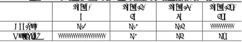
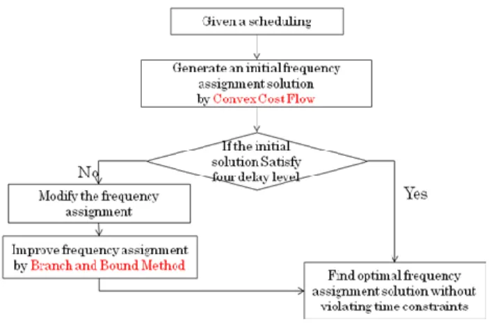
(2) Vol.2010-SLDM-145 No.3 2010/5/19. 情報処理学会研究報告 IPSJ SIG Technical Report. is easy and flexible to search the design space; (3) allows to make decisions at early stage of the design cycle and to balance the degree of freedom for power optimization. Some algorithms have been studied before; see [7, 8, 9] and references therein. In [7], ILP-based scheduling attempts to minimize the energy and delay product. In [8], the authors studied this problem in which a heuristic algorithm was proposed which scheduled lower frequency operators at earlier steps and delays higher frequency operators to later steps. The ILP-based scheduling can obtain an optimal solution but not effective. For the heuristic method in [8], the solution space is not large enough to search a desired solution. In this paper, we propose a new method, which combine the convex cost flow and branch and bound method to solve frequency assignment problem for the given scheduling. The objective is to reduce the power dissipation as much as possible taking account of timing constraints We apply convex cost flow network and branch and bound method was used to assign the frequency for each control step of the scheduling. The rest of the paper is organized as follows. Section 2 gives the formulation of frequency assignment. Section 3 discusses the feasible solution obtained by the convex cost flow network flow. Section 4 gives the frequency adjustment method based on the branch and bound method with upper and lower bounds. Experimental results are shown in Sect.5. Finally, Sect.6 concludes the work.. 2.. of the control steps to support the application of MVDF technology. The objective is to minimize the total energy cost by assigning different frequencies to control steps without violating the timing. Given a scheduling S, with n control steps C j, j=1, 2 … n. Different control steps may work in different frequencies, f base, fbase/2i, i=1, 2 … m. In order to simplify the expression, we replace the frequency f to be delay d (d=1/f). So, there are m delay levels in set D which denotes by d i, i=1, 2 …m; d ij is the latency level i of control step j; the energy dissipation associated with delay level i of control step j can present as. E j (d ij ) According to the definition and notation above, the frequency assignment problem can be easily formulated into the following fu nction:.  iD, jC E j (dij ) to  iD, jC dij  Tc. Minimize subject. The timing constraint of the scheduling is T c. We can also get a table about the dynamic frequency and energy dissipation of the Units, such as table 1. Table 1. Problem Formulation. As the introduction above, in multiple voltage and dynamic frequency scheme, a clocking mechanism that varies the clock frequency dynamically should be generated. We assume the base frequency (fbase) which is the maximum frequency of any function unit at the maximum supply voltage Assume the dynamically operating frequency as fdynamic. The detail is introduced in [7] .. fdynamic  fbase / 2n. 3.. The target architecture model assumed in the design of scheduling schemes is showed in Figure 2. Value n is loaded as an input to the DCU which comes from controller. By fbase and n, this Dynamic Clocking Unit uses a clock divider strategy to generate dynamic frequency fdynamic. See [2]. dynamic frequency and energy dissipation of the units (fbase). (fbase/2). (fbase/4). d. 2d. 4d. (fbase/2n) 2nd. Add/Sub. E’0. E’1. E’2. -----------. Multiplier. ----------------------. E1. E2. En. Initial Solution based on Convex Cost Flow Algorithm. In this section, we consider this frequency assignment problem with convex function so as to minimize the total energy consumption while still guarantee satisfaction of all timing constraints. And then improve the initial solution by branch and bound method. The main flow is shown in Figure 3. Convex cost flow problems are minimum cost flow problems where the cost of flow is nonlinear. The convex cost flow can be apply to a number of existing solutions. One possible way is to reduce the problem to a typical linear cost flow problem using piecewise linearization of the arc cost functions.. Figure 2 Dynamic frequency generation mechanism As the discussion above, given a scheduling, I concern the frequency assignment problem 2. ⓒ2010 Information Processing Society of Japan.

(3) Vol.2010-SLDM-145 No.3 2010/5/19. 情報処理学会研究報告 IPSJ SIG Technical Report. constant cost network which can be solved by min-cost max-flow algorithm. The transition of one control step with multipliers is shown in Figure 5.. Figure 4 Figure 3 Main Flow We summarize this method into three steps:  Construct convex cost flow network  Calculate convex cost flow function of each control step.  Transform this convex cost flow to a minimum cost flow problem , and then solve it using the cycle canceling algorithm 3.1 Convex cost network construction Given a scheduling with a set of n control steps C 1, C2, C3 … Cn, each control step may work in delay levels d1, d2, d3 … d m. Ej(d ij) is convex cost function of energy dissipation associated with delay level i of control step j. We can obtain the dynamic frequency and Energy dissipation of each control step due to the Function unit table. There maybe two cases in each control step. (1) Only one type resource in one control step, we consider the proposed dynamic frequency and energy dissipation of this type. (2) Both multipliers and adders in one control step, we just consider the frequency of multipliers. A flow network is constructed by adding a source node S, a node o, and a sink node t to control step node set C，and one edge (s, o), two edge sets { (o, c j) | cj∈C}∪{(cj, t) | cj∈C}. The capacity of the incoming edge of node o is according to the time constraint T c. The capacity of other edges is ∞. The cost of the edge set {(o, cj) | cj∈C} is a convex cost according to E ij (d ij), the cost of other edges is zero. The constructed convex cost network is shown in figure 4.. Figure 5. Convex cost Flow Network. convex cost flow of control step 1 with multiplier. 3.2 Convex-cost Function. According to the delay and energy value in table 1, we can easily construct piecewise linear convex cost functions of each type operation. Different types of operations operate in different delay level. The energy-delay trade-off of different types of operations is represented by a delay-energy curve. First, due to the delay values and energy dissipation of function units, vectors (E(d i), d i) can be obtained. The energy consumption can be explicitly represented in y-axis; the latency can be represented in x-axis. Connect the above vertices in sequence, we obtain a simple piece-wise linear diagram indicates the trade-off between energy and frequency. And then easy to construct the convex flow function of each control step of the given scheduling. Just take type adder as an example. In this piecewise linear function, according to delay and energy consumption of adders, we connect the vectors {(1, E0), (2, E1), (4, E2)… (2n, En)}.. The unit flow cost of the convex function can change along with the number of flows. Therefore it is so difficult to get the solution straightly that we have to change it to a 3. ⓒ2010 Information Processing Society of Japan.

(4) Vol.2010-SLDM-145 No.3 2010/5/19. 情報処理学会研究報告 IPSJ SIG Technical Report. convex function of adder and multiplier unit. Figure 7 shows the convex function of the control step with two multipliers. Figure 5. piecewise convex cost function. 3.3 Example used in industry. Due to the voltage levels that these are used in industrial design, the frequency discussed in this paper is changed dynamically and the supply voltage is assigned from one of the available levels (5.0V, 3.3V, 2.4V).Table 2 and Table 3 show the Energy dissipation and delay when the components are operated in available levels. See [8]. Different type operations have three different delay choices under the supply voltage 5v, 3.3v, 2.4v. We assume the base delay is 1d when using the base frequency. Due to Table 2 and Table 3,  For adders and substracters, the delay level is 1, 2, and 4.  For multipliers, the delay level is 2, 4, and 6. Table 2 Energy dissipation of functional units Component. Energy (5v). Energy (3.3v). Add/Sub. 57pJ. 25pJ. 13pJ. Multiplier. 2202pJ. 960pJ. 507pJ. Table 3 Component. Add/sub. Maximum Freq Scaled Down Freq Multiplier Maximum Freq Scaled Down Freq. Figure 6. Delay（5V） 35.0ns. Delay（3.3V） 62.2ns. Delay（2.4V ）. 28MHz. 14MHz. 7MHz. 63.3ns 15.8MHz 14MHz. 16.07MHz 113.3ns 8.82MHz 7MHz. (a) add/sub. (b) multiplier. Energy (2.4v). Figure 7 Convex function--control step with two multiplier 3.3.2 Construct flow network Figure 8 shows the construction of the cost flow network.. Delay values and clock frequencies. 28.5MHz. Convex function for flow cost. 105.3ns 9.49MHz. Ei1 (d1i ). 192.2ns. Ei 2 (d2i ). 5.2MHz 4.6MHz. Ei3 (d3i ). 3.3.1 Construct convex cost piece linear function of each control step. Figure 6 shows the. Figure 7. An example of given scheduling and convex cost flow network. 4 ⓒ2010 Information Processing Society of Japan.

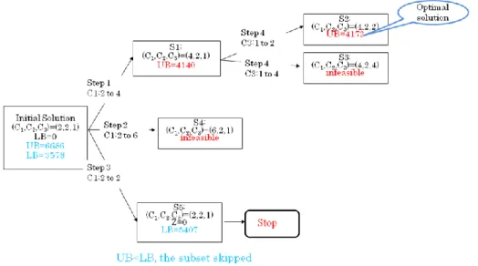
(5) Vol.2010-SLDM-145 No.3 2010/5/19. 情報処理学会研究報告 IPSJ SIG Technical Report. 3.3.3 Solve the convex cost flow problem. We may get two cases as figure 9. Case (a) is a. Minimize. desirable solution; case (b) is a solution which need improvement.. E x.  E0   E s i xi. s x. T. iC. Subject to. iC. i i. i i. iC. T  Tc  T0. xi   0,1 i  N  0  i  1. Where E0 is the energy of the initial solution, E s is the energy saving. Tc is the timing constraints, T0 is the total time used in the initial solution. The relaxation problem can easily be solved as follows: For each commodity, calculate the value per clock cycle vi/si. Take in the descending order of v i/si, such as the example shown in Table 3. Table 3 descending order calculation C1 C2 C3 V1 to V2 V1 to V2 V1 to V2/V3 Value (Energy saving) 2484 1247 32/12 Size (Time ) 2 2 1/2 Value/Size 1242 624 32/6. (b) (a) Figure 9 Initial assignment 3.4 Assignment Modification However, when the solutions we get from the convex cost flow algorithm does not satisfy the delay level we talked about, a modification of delay levels should be discussed. In order to not violate the latency, the delay after the modification should smaller than the previous. So, we change delay level 3 to level 2, delay level 5 to level 4. An example is shown in figure 10.. 4.2 Branching and bounding rules. Figure 10. 4.. We divide the large problem into several subproblems. The branching rules are remaining the current delay level and Updating initial delay level to higher delay level. UB is equal to the objective function will not exceeds this value; LB is calculate from the objective function that will not be less than this value. The upper bound is the energy consumption in our problem. With the upper and lower bounds obtained above, we can construct our pruning rules. We cannot find a feasible solution satisfying the timing constraint even assuming a continuous domain for the module voltages, we will prune. If a node`s lower bound is greater than or equal to the global upper bound, it will also be pruned. Due to the branching and bounding rules, we can get the solution of the example in figure 11. In this example, the upper and lower bound in the initial solution: UB0=E1+E1+E’0=2202*2+ (2202+25) + 57=6686 LB0=6686-2484-1247/2=3578. In subset 2, UB2=E2+E1+E’1=960*2+ (2202+25) +25=4172, this solution is better than the initial solution. In subset 5, LB5= 6686-1247-32=5407. The lower bound is bigger than UB 2, we pruned this subset.. Assignment Modification. Assignment Improvement based on the branch and bound method. 4.1 Branch and bound function formulate. The initial solution based on the convex cost flow algorithm may be not the optimal solution because of the frequency assignment modification. Branch and Bound is by far the most widely used tool for solving large scale optimization problems, especially in discrete optimization. Since the original “large” problem is hard to solve directly, it is divided into smaller and smaller subproblems until these subproblems can be conquered. Because it is difficult to find a good and small upper bound, we exploit a linear relaxation of the problem. The optimal solutions of a relaxation problem may not be integers. Then the problem can be defined as the follows, 5. ⓒ2010 Information Processing Society of Japan.

(6) Vol.2010-SLDM-145 No.3 2010/5/19. 情報処理学会研究報告 IPSJ SIG Technical Report. 4) M. Sarrafzadeh and S. Raje: Scheduling with Multiple Voltages under Resource Constraints, Proc. of ISCAS’99, pp. 440-445 (1999). 5) N. Ranganathan, N. Vijakrishnan, and N. Bhavanishankar: A VLSI Array Architecture with dynamic frequency clocking, Proc. of ICCD’96, pp.137-140 (1996). 6) M. Johnson and K. Roy, Datapath Scheduling with Multiple Supply Voltages and Level Converters, ACM Trans. on Design Automation of Electric Systems, Vol.2, No.3, pp. 227-248 (1997). 7) S. P. Mohanty: Low-Power High-Level Synthesis for Nanoscale CMOS. 8) Saraju P. Mohanty, N. Ranganathan, V. Krishna: Datapath Scheduling using Dynamic Frequency Clocking, Proceedings of the IEEE Computer Society Annual Symposium on VLSI (2002). 9) Saraju P. Mohanty and N. Ranganathan: Energy-efficient datapath scheduling using multiple voltages and dynamic clocking. ACM Trans. Des. Autom. Electron. Syst. 10, 2 (2005).. 著者紹介. Ru, LIU. Figure 11. 5.. received the B.S. degree in Electronic Engineering from Dalian University of Technology, China, in 2008. She is currently working toward the M.E. degree in LSI system at the Graduate School of IPS, Waseda University, Japan. She main research interest is behavior design for VLSI, primarily in the area of scheduling. Song, CHENG（Member） received the B.S. degree in computer science from Xi'an Jiaotong University, Xi'an, China, in 2000, the M.S. and Ph.D. degrees in computer science from Tsinghua University, Beijing, China, in 2003 and 2005, respectively. He is currently a visiting lecturer at the Graduate School of IPS, Waseda University, Japan. His research interests include several aspects of electronic design automation, e.g., floorplanning, placement and high-level synthesis. Takeshi, YOSHIMURA（Fellow） received B.E., M.E., and Dr. Eng. degrees from Osaka University, Osaka, Japan, in 1972, 1974, and 1997. He joined the NEC Corporation, Kawasaki, Japan, in 1974, where he has been engaged in research and development efforts devoted to computer application systems for communication network design, hydraulic network design, and VLSI CAD. From 1979 to 1980 he was on leave at the Electronics Research Laboratory, University of California, Berkeley, where he worked on very large scale integration computer-aided design layout. He received Best Paper Awards from the Institute of Electronics, Information and Communication Engineers of Japan (IEICE) and the IEEE CAS Society. Dr. Yoshimura is a Member of the IEICE, IPSJ (the Information Processing Society of Japan), and IEEE.. the result solution of Branch and Bound. Conclusion. The MVDFS problem concerns how to optimally assign frequency of the control steps so that the total energy cost is minimized, where the latency not violate the timing constraints and different control step has different delay level as we talked about. This paper presents a convex cost and branch and bound based algorithm which provides efficient frequency assignment solutions for the multiple voltage and dynamic frequency scheme. The experimental results demonstrate that the proposed algorithm can effectively solve multiple voltage and dynamic frequency problem.. 参考文献 1) M. Pedram: Power Minimization in IC Design: Principle and Applications, ACM Trans. on Design Automation of Electric Systems, Vol.1, No.1, pp. 3-56 (1996). 2) J. M. Chang and M. Pedram: Energy minimization using multiple supply voltages, IEEE Trans. On VLSI Systems, Vol.5, No.4, pp.436-443 (1997). 3) A. Kumar and M. Bayoumi: Multiple Voltage-Based scheduling Methodology for Low Power in the High Level Synthesis. Proc. of ISCAS’99. Pp.371-379 (1999).. 6 ⓒ2010 Information Processing Society of Japan.

(7)