Panel Data Research Center, Keio University
PDRC Discussion Paper Series
利用しすぎると、すべてを失うか? 労働時間の健康への影響について
梶谷真也、マッケンジー コリン、坂田圭
2020 年 2 月 3 日
DP2016-009
https://www.pdrc.keio.ac.jp/publications/dp/1240/
Panel Data Research Center, Keio University
2-15-45 Mita, Minato-ku, Tokyo 108-8345, Japan
[email protected]
3 February, 2020
利用しすぎると、すべてを失うか? 労働時間の健康への影響について 梶谷真也、マッケンジー コリン、坂田圭
PDRC Keio DP2016-009 2020 年 2 月 3 日
JEL Classification: I10, J2
キーワード: 健康;労働時間;内生性;年金;定年退職 【要旨】 ・40歳以上のオーストラリア人の男性について労働時間と健康との間の非線形関係を調べ た。 ・ゼロ時間から労働時間を増やすと、健康へ正の影響を与えるが、良い影響のピークは 週当た り 24ー27 時間となる。それ以上に、働くと正の影響が減る。 ・働かない場合に比べて、週当たり 50 時間働くと、健康への影響がだいたい体同じである。 梶谷真也 京都産業大学経済学部 〒603-8555 京都府京都市北区上賀茂本山 [email protected] マッケンジー コリン 慶應義塾大学経済学部 〒108-8345 東京都港区三田2-15-45 [email protected] 坂田圭 [email protected]
1
Use it Too Much and Lose Everything? The Effects of
Hours of Work on Health
Shinya Kajitania, Faculty of Economics, Kyoto Sangyo University
Colin McKenzieb, Faculty of Economics, Keio University
Kei Sakatac, Australian Institute of Family Studies
Acknowledgements
The authors would also like to thank Daiji Kawaguchi and participants at the following workshops and conferences, the Ageing and Longevity in the UK and Japan: Perspectives from the Health and Social Sciences Workshop (King’s College London), the Globalization and the Building of a High Quality Economic System Conference (Keio University), the 10th
International Conference of the Thailand Econometric Society 2017 (Chiang Mai University), the 22th Euroasia and Business and Economics (EBES) Society Conference (Sapienza
University of Rome), the 2019 Gerontological Society of America Annual Scientific Meeting (Austin, Texas), and the Spring Conference of the Japanese Economic Association (Ritsumeikan University) for their helpful and constructive comments on earlier versions of this paper. This paper uses unit record data from the Household, Income and Labour Dynamics in Australia (HILDA) Survey. The HILDA Project was initiated and is funded by the Australian Government Department of Social Services (DSS) and is managed by the Melbourne Institute: Applied Economic and Social Research, the University of Melbourne (the Melbourne Institute). The findings and views reported in this paper, however, are those of the authors and should not be attributed to DSS, the Melbourne Institute, or the Australian Institute of Family Studies.
Declarations
The authors declare they do not have any actual or potential conflict of interest in relation to this research. No ethic approval was required for this study.
Funding
This research was supported by the Japan Society for the Promotion of Science (JSPS) Grant
aShinya Kajitani, Faculty of Economics, Kyoto Sangyo University, Motoyama, Kamigamo,
Kita-ku, Kyoto City 603-8555, JAPAN. Email: [email protected]
b Corresponding author: Colin McKenzie, Faculty of Economics, Keio University, 2-15-45
Mita, Minato-ku, Tokyo 108-8345, JAPAN. Email: [email protected]
c Kei Sakata, Australian Institute of Family Studies, Level 4, 40 City Road, Southbank,
2
in Aid for Scientific Research (B) No. JP24330093 for a project on “Retirement Behaviour of the Aged and their Cognitive Ability and Health” (P.I.: Kei Sakata), a Japan Society for the Promotion of Science (JSPS) Grant in Aid for Scientific Research (B) No. 16H03607 for a project "An Empirical Analysis of Parental Employment Status, Time Allocation and Way of Thinking, and their Children's Human Capital Formation" (Project Leader: Midori Wakabayashi), and Kyoto Sangyo University Research Grant No. E1901 (P.I.: Shinya Kajitani).
3 ABSTRACT
The “use it or lose it” hypothesis examines whether active involvement in work can prevent cognitive decline for elderly workers, but how much work is good for health is as yet unknown. We examine the causal impact of working hours on various health outcomes of Australian men aged 40 years and over using panel data from the HILDA survey over the period 2001 to 2012. To capture the potential non-linear dependence of health status on working hours, the models for health outcomes include working hours and its square as explanatory variables. We deal with the potential endogeneity of working hours by using the instrumental variable estimation technique with instruments based on the age for pension eligibility. There is time series variability in the pension eligibility ages for some men because in 2009, significant changes in pension eligibility ages were announced for some, but not all males. A non-linear causal effect of working hours on health is confirmed. For males working relatively moderate hours (up to around 24–27 hours for a week), an increase in working hours has a positive impact on health, but thereafter an increase in working hours has a negative impact on health.
Keywords: health, working hours, endogeneity, pensions, retirement. JEL Classification Nos: I10, J2
Highlights
For Australian men aged 40 years and over, a non-linear causal relationship between working hours and health is observed.
Moderate hours of work provide health benefits, and these benefits peak around 24–27 hours of work for a week. The positive health effects decline after the peak of 24–27 hours of work, and around 50 hours of work all the positive effects of work disappear. Working slightly more than 50 hours leads to health outcomes that are worse than
4 1. Introduction
How does work affect health? Is work bad for health? Does work have any health benefits? There is an extremely large literature in epidemiology, occupational psychology, and health economics that examines these issues (see, for example, Bannai and Tamakoshi, 2014, Bassanini and Caroli, 2015). Some papers examine the extensive margin of work (working or not working), for example, by examining the impact of unemployment and job loss on health outcomes. Using fixed-effect models for Australian, Canadian and UK panel data, Llena-Nozal (2009) shows that the shift from being employed to being unemployed has adverse effects on mental health. On the other hand, using German data, Schmitz (2011) finds no significant effect of plant closures on various health outcomes. Heller-Sahlgrem (2017) finds no immediate effect, but rather a delayed impact of retirement on mental health. Another stream of research on the extensive margin examines whether retirement has any impact on cognitive functioning and health. Such studies test the so-called “use it or lose it” hypothesis (Rohwedder and Willis, 2010, Coe and Zamarro 2011, Bonsang et al. 2012, De Grip et al. 2012, Mazzonna and Peracchi 2012, Blake and Garrouste 2017, Kajitani et al. 2017a, Mazzonna and Peracchi 2017, Atalay et al. 2019). Overall, these studies tend to suggest that retirement has a negative impact on cognitive functioning, but positive impacts on health outcomes.
Other papers examine the intensive margin of work, that is, the number of hours worked. The main focus of these analyses is on the effects of working long hours on various health outcomes. Such studies reveal that working long hours has adverse effects on health (Spurgeon et al. 1997, Sparks et al. 1997, Frijters et al. 2009, Bannai et al. 2015, Nie et al. 2015). In a paper that emphasises the importance of employment policy in Europe in the context of the relationship between work and health, Barnay (2016) argues that while there is a large literature in epidemiology on the intensive margin of work on health outcomes, there is next to no literature in economics (see also Bannai and Tamakoshi 2014). Lee and Lee (2016) examine the impacts of working hours on injury rates at the worker’s workplace which is regarded as one of the risk factors for their health, exploiting a quasi-natural experiment in South Korea. Assuming that the injury risk is a quadratic function of working hours, they find that the function is convex, which indicates that shortening very long working hours could be effective in reducing the injury rate. However, previous studies do not examine the effects of moderate working hours on health or the optimal number of hours worked. Robone et al. (2011) indicate that having a part-time job, as compared to a full-time job, has a positive impact on the health of people who are satisfied with their working hours. For males, Llena-Nozal (2009) finds that compared to working full-time, working overtime leads to a worsening of mental health outcomes1. This highlights the fact that the relationship 1 In contrast, for women, Llena-Nozal et al. (2004) find that compared to working full-time,
5
between work and health may not be linear. Work can be a double-edged sword in that it can have both positive and negative effects. Interactions with people at work may help maintain an individual’s cognitive functions and his/her mental health. Moreover, working individuals have more incentive to invest in health repair activities in order to be ‘fit’ in the labour market. On the other hand, long working hours can cause fatigue and stress on both physical and mental levels which potentially damage an individual’s overall health and also reduce the amount of time that can be investment in health repair activities. Most of the previous studies treat long working hours as a 0–1 dummy variable which defines long working hours as working more than 50 or 60 hours per week. This means that they implicitly assume that long working hours have a constant shift effect on health status. They do not deal with the potential non-linear effects of working hours on health.
For health outcomes, the literature on the extensive margin suggests that working may be better than not working, while the literature on the intensive margin suggests that working extremely long hours is worse than working a normal working week. Combining these two observations suggests there is a non-linear relationship between workhours and health outcomes which we seek to capture using a quadratic form in workhours. Although not directly focusing on health outcomes, one explanation for the results generated in Pencavel’s (2014, 2016) analysis of the nonlinear relationship between working hours and productivity in munitions factories in Britain during the First World War is stress and fatigue generated by long working hours that then affects productivity (see also Collewet and Sauermann, 2017).
We contribute to the existing literature in two ways. First, we focus on not only labor market participation (the extensive margin), but also working hours (the intensive margin). Secondly, the literature examining the impact of retirement on cognitive function examines the ‘use it or lose it’ hypothesis, namely that not working (not using your brain) leads to losses of cognitive functioning. Here, we also examine the relevance of this hypothesis for a broader set of health outcomes. In addition, we focus on the ‘use it too much and lose everything’ hypothesis which refers to the situation where working too much can lead to not just a loss of cognitive functioning (see Kajitani et al. 2017b), but also declines in health status across the board.
We examine the causal impact of working hours on the health outcomes of middle-aged and older male adults (men aged 40 years and over) in Australia using Wave 1 to Wave 12 of the Household, Income and Labour Dynamics in Australia (HILDA) Survey. The health outcomes are measured using five self-assessed health score components computed from the SF-36 (the 36-Item Short Form Health Survey) which is one of the most widely used self-assessed measures of health status. These score components cover both an individual’s moving to part-time work or overtime lead to improvements in mental health outcomes.
6
physical and mental health (see Ware, 2000). One of the issues in estimating the causal relationship between hours worked and health is what is called the ‘healthy worker effect’ (Bassanini and Caroli, 2015), that is, healthy workers are more likely to be employed and work longer. Thus, the presence of the healthy worker effect implies the existence of reverse causality. We deal with the potential endogeneity of decisions relating to working hours by using the instrumental variable estimation technique. One advantage of using a sample of middle-aged and older adults is that it enables us to use information related to the eligibility age for pension benefits as instruments for variables related to working hours.
Our empirical evidence shows that there is non-linearity in the effects of working hours on self-assessed health status. To be more specific, there is an inverted U-shaped relationship. When working hours are less than around 24–27 hours a week, increases in working hours have a positive impact on health. However, when working hours are greater than this threshold, increases in working hours have negative impacts on health. Compared to males who do not work, working hours slightly over 50 hours will lead to worse health outcomes depending on the measure of health status. These results suggest that men in old age could maintain or improve their health status ability compared to not working by working in a part-time job that requires them to work around 24–27 hours per week. The results are consistent with the analysis on cognitive functioning of Kajitani et al. (2017b).
The rest of this paper is organized as follows: Section 2 provides a brief description of the Australian pension system. Section 3 presents the empirical framework used in this paper. Section 4 describes the data, and Section 5 reports the results of estimation and discusses their implications. The last section concludes this paper.
2. Australian pension system
In Australia, the timing of retirement is closely related to the pension system. Retirement income consists of three sources: a means tested public pension, a mandatory employer-contributed private retirement savings account, and voluntary private retirement savings. Since there is no mandatory retirement age in Australia, an elderly Australian can also continue to work to supplement his/her pension.
The maximum benefit payment from the public age pension is set at 25% of male total average earnings. Since the introduction of the good and service tax in 2000, a supplement for compensation has been added to the payment. The maximum basic rates of the public pension were A$10,262.20 per annum for the standard rate and A$8,569.60 per annum for the partnered rate in September 2001. In September 2012, at the time of HILDA Wave 12, the maximum standard rate had been increased to A$ 18,512.00 and the partnered rate to A$ 13,954.20. It is important to note that the maximum benefit is subject to both an income test and an asset test (for details see Atalay and Barrett, 2015).
7
residency condition, individuals are required to have been resident in Australia for at least ten years. The aged pension eligibility age for males was set at 65 in 1909. In June 2008, a little over 80% males and females aged 65 or over were receiving aged pensions (Hammer (2008, Chart 20)). In 2009–10, ABS (2011, Table 3) estimates that for 59.2% of those people receiving the aged pension the government pensions and allowances contributed to more than 90% of their gross household income. That is, for a large number of Australians the aged pension provides an important source of income.
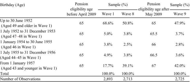
On 12 May 2009, Wayne Swan, the Treasurer, and Jenny Macklin, the Minister for Families, Housing, Community Services and Indigenous Affairs, jointly announced that starting in 2017 the qualifying age for the aged pension for males would be gradually increased from 65 to 67 by 20232. As can be seen from Table I, this policy change raised the
pension eligibility ages for males in the “younger” generations from 65 to 65.5, 66, 66.5 or 67 depending on their birthdates. For males born before or on 30 June 1952, there was no change in their pension eligibility age. We will use variations in the pension eligibility age to identify the labour supply behavior of the middle age and elderly male workers in Australia.
[Table I around here] 3. Estimation model and identification strategy
Our identification strategy exploits the variation in working hours, while controlling for time-invariant individual characteristics. In order to capture the possible non-linear effects of working hours on health status, we consider the following model for health outcomes3:
𝑦 = 𝛼 + 𝛼 𝑊𝐻 + 𝑋1 𝛽 + 𝑢 , 𝑖 = 1, . . 𝑁, 𝑡 = 1, . . , 𝑇 (1a)
𝑢 = 𝜇 + 𝜖 (1b)
where 𝑦 denotes various health outcomes (physical functioning, bodily pain, general health, vitality, and mental health) for individual 𝑖 at the time of the survey 𝑡, and 𝑊𝐻 is working hours. In estimating equation (1a), we include those individuals whose working hours are zero. 𝑋1 denotes a vector of time variant control variables: a spouse 0–1 dummy
2 The joint press release is available from the following URL:
http://ministers.treasury.gov.au/DisplayDocs.aspx?doc=pressreleases/2009/056.htm&pageI D=003&min=wms&Year=2009&DocType=0 (Accessed 30 June 2019)
3 An alternative to the parametric model in equation (1a) to account for the non-linear effect
of working hours on health status would be to estimate a semi-parametric or non-parametric model. However, such an approach makes it rather difficult to deal with the potential endogeneity between working hours and health status. Here, we put priority on dealing with the potential endogeneity of working hours.
8
variable, Married, which takes the value one if the respondent has a spouse and zero otherwise; the number of dependent children, Number of dependent children; the respondent’s age, Age, which controls for age-related effects; and a house ownership 0–1 dummy variable, Ownhouse, which indicates whether the respondent owns or is in the process of owning his house as a proxy for assets. The variables related to the respondent’s marital status and the number of dependent children are included because communication and interaction with other family members may prevent declines in health, particularly in mental health. In addition, the number of dependent children is included since it can be argued that people with dependent children may be likely to invest more in their health capital. The house ownership dummy is included to control for the effects of assets holdings on health. In addition, 𝑋1 includes four 0–1 regional dummies. 𝑁 is the number of individuals and 𝑇 is the number of observations available for individual 𝑖 indicating that we have an unbalanced panel. As equation (1b) indicates, 𝑢 is an error term which consists of a time invariant individual fixed effect, 𝜇 , and an idiosyncratic error, 𝜖 , so that we allow for some degree of individual heterogeneity. The coefficients 𝛼 and 𝛼 in equation (1a) capture the non-linear effect of working hours on a health outcome. Given the discussion in section 1 that some work is better than no work, and that too much work may be worse than some work, it is expected that 𝛼 < 0 and 𝛼 > 0. Holding everything else constant, it is easy to see that the value of a health score is maximized when 𝑊𝐻 = −𝛼 /(2𝛼 ) , and that for 𝑊𝐻 = −𝛼 /𝛼 the level of health is the same as it would be if the respondent is not working.
The possibility of the endogeneity of the respondents’ working hours in equation (1a) is a major obstacle to estimate the causal impact of working hours on health. As discussed in section 1, this particular identification problem is called the ‘healthy worker effect’, that is healthy individuals are more likely to be employed and to work longer whereas unhealthy workers may decide to leave the workforce or work short hours. Individuals, who are healthier and, therefore, tend to earn a relatively higher wage, could decide to reduce their hours of work. The same logic can be applied to health outcomes.
In order to account for the potential endogeneity of working hours and its square in equation (1a), we use an instrumental variable estimator using two instruments, Age difference 1 and Age difference 2, that are based on pension eligibility ages. These instruments measure the distance from an individual’s retirement age. More specifically, Age difference 1 is the difference between a respondent’s age and the respondent’s pension eligibility age provided the respondent has reached the eligibility age and zero otherwise, while Age difference 2 is the difference between a respondent’s age and the respondent’s pension eligibility age provided the respondent has not reached the eligibility age and zero otherwise. That is, we assume with the following models:
9
𝑊𝐻 = μ 𝐴𝑔𝑒 𝑑𝑖𝑓𝑓𝑒𝑟𝑒𝑛𝑐𝑒 1 + μ 𝐴𝑔𝑒 𝑑𝑖𝑓𝑓𝑒𝑟𝑒𝑛𝑐𝑒 2 + 𝑋1 μ + 𝑤 , (2) 𝑊𝐻 = μμ 𝐴𝑔𝑒 𝑑𝑖𝑓𝑓𝑒𝑟𝑒𝑛𝑐𝑒 1 + μμ 𝐴𝑔𝑒 𝑑𝑖𝑓𝑓𝑒𝑟𝑒𝑛𝑐𝑒 2 + 𝑋1 μμ + 𝑤𝑤 , (3) where the error terms, 𝑤 and 𝑤𝑤 , include individual fixed effects.
As can be seen from Table I, in our sample, a reasonable amount of variation in the eligibility age is observed. Although the pension eligibility age for men remained at the age of 65 for individuals born before or on 30 June 1952, the proportion of this group in Wave 9 (just after the 2009 pension reform) is just 47.9%. The proportion of men whose pension eligibility age is 67 in Wave 9 consists of 42.0%.
[Table I around here]
The two instruments in equations (2) and (3) are closely related to one of the standard instruments used for the analysis of the causal relationship between retirement and cognitive functioning (Atalay et al. 2019, Bonsang et al. 2012, Coe and Zamarro 2011, Mazzonna and Peracchi 2012, Mazzonna and Peracchi 2017, Rohwedder and Willis 2010). It is worth pointing out that, in the literature that tries to determine the causal impacts of retirement on health outcomes, these pension related instruments are used to explain the retirement decision, that is, the extensive margin, not the number of hours worked.
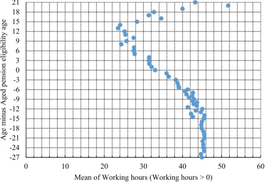
Here we rely on Neumark and Powers (2000, 2003/4, 2005, 2006), Kudrna and Woodland (2011a,b) and Vere (2011) to justify using these pension eligibility age related variables as instruments for also explaining the intensive margin of working hours as well. Neumark and Powers (2000, 2003/4, 2005, 2006) provide a theoretical explanation of the connection between social security in the United States and hours worked prior to retirement, while Vere (2011) provides some empirical evidence for the US on the connection between pension payments and hours worked. In the context of a dynamic general equilibrium model, Kudrna and Woodland (2011a,b) provide evidence for Australia on the effect of the major reform of the Australian pension system that was announced by the Australian Government in the 2009/2010 national budget that we are considering on working hours. Furthermore, in the data set we are using for individuals who report their working hours are positive, Figure I graphs the relationship between the average of working hours and the difference between a respondent’s age and pension eligibility age. For values of this difference less than 10, there would appear to be a negative relationship between this variable and the average of working hours4. One reason for limiting our sample to males aged 40 and over is to ensure that there
4 For values of Age minus Aged pension eligibility age greater than or equal to 15, the sample
size to compute each average is rather small (less than 10), so that the estimation of the average is not so precise.
10
is a sufficient connection between the changes in pension eligibility ages and working hours. [Figure I around here]
In both equations (2) and (3), the dependent variable is non-negative, but Wooldridge (2010, p. 90) makes the important point that the application of instrumental variable (IV) estimator is not limited to the case where the dependent variable(s) in the first stage is (are) continuous, so even though working hours are non-negative this is not an impediment to the application of the IV technique.
4. Data: Overview of the HILDA Survey
Our data are drawn from the first 12 waves of the “Household, Income and Labour Dynamics in Australia (HILDA) Survey,” from Wave 1 conducted in 2001 to Wave 12 conducted in 2012. The HILDA Survey which is conducted by the Melbourne Institute: Applied Economics and Social Research, the University of Melbourne is a broad social and economic longitudinal survey. Since 2001, the HILDA Survey has asked Australian respondents about their economic and subjective well-being, family structures, and labor market dynamics. Household included in the survey were selected using a three-stage approach. First, a sample of 488 Census Collection Districts (CDs) were randomly selected from across Australia. Second, within each of these CDs, a sample of dwellings was selected based on expected response rates and occupancy rates. Finally, within each dwelling, up to three households were selected to be part of the sample. In addition, the sample was replenished in Wave 11. One aim of this replenishment was to provide better coverage of migrants for inclusion in the HILDA Survey5.
The HILDA survey contains the SF-36 (the 36-Item Short Form Health Survey) which is one of the most widely used self-assessed measures of health status6. It consists of eight
scaled self-assessed health scores: physical functioning; role physical; bodily pain; general health; vitality; social functioning; role emotional and mental health. The eight categories are scaled by the weighted sums of their questions, and are converted to a 0–100 scale. 0 is equivalent to the highest disability, and 100 is equivalent to the lowest disability7. Of the 5 Detailed information on the sample design of the HILDA Survey is available in Wooden et
al. (2002) and Watson and Wooden (2013).
6 Cai and Kalb (2006) in an analysis of the SF-36 data in HILDA report some discrepancies
in health status when it is self-reported compared to when the data is obtained through interviews.
7 Although each self assessed health score is bounded from below by zero and above by 100,
and there are individuals who score one of these two boundary values (see Table II), we do not employ a double sided Tobit type estimator when estimating equation (1a).
11
eight health scores, we use physical functioning, bodily pain, general health, vitality, and mental health. The other three scores, role physical; social functioning; and role emotional, are eliminated from the analysis because they display little variation.
The general release HILDA data sets that we are using do not contain information on the day or month of birth of the respondent. In each wave, for each individual two ages are reported: the age as at 30 June of the year of the wave, and the age at the time of the survey. Using information on the age of respondents as at 30 June in the first wave it is possible to determine the pension eligibility ages of all individuals except those whose age is reported to be 44 and 47 in this wave. Using both ages and the information on when the respondent was interviewed, it is possible to determine the pension eligibility age for 25% and 32% of those respondents whose ages are reported to be 44 and 47 at 30 June 2001 in wave 1, respectively. Those respondents whose pension eligibility age could not be determined were excluded from the analysis. Table O1 in the online supplementary material indicates the impact of this exclusion on the sample size available in each wave.
As stated in section 2, the 2009 pension reform was announced on 12 May 2009. As the interview periods for HILDA’s waves 8 and 9 are from 20 August 2008 to 27 February 2009 and from 20 August 2009 to 11 March 2010, respectively, the 2009 pension reform falls right between waves 8 and 9.
The exact definitions of all the variables used in the analysis in this paper are summarized in Appendix I. The sample is restricted to individuals who meet the following five criteria: (i) males aged 40 and over in Wave 1 of the survey or males who turn 40 after Wave 1 but are only included for the Waves where they are aged 40 and over; (ii) all five scores relating to health status are available; (iii) age and working hours are less than age and working hours in the top 1% percentile, respectively; (v) respondents who report they are unemployed are excluded; and (v) information on all the relevant variables is available. We target this age group as people start experiencing some health declines. For example, the Australian Heart Foundation recommends that people over 45 (over 35 for Aboriginal and Torres Strait Islanders) have a heart health check8 . The National Bowel Cancer Screening Program is
offered to all Australians aged 50 – 74 in 20209. In addition, this sample selection is applied
for our identification strategy as younger age groups are thought to be indifferent to changes in their retirement age. Even if we did not have attrition, the second part of criterion (i) means we will not have a balanced panel data set. After imposing these restrictions, a sample of 35,196 observations on 6,022 individuals remains. Table O1 in the online supplementary
8 See, for example,
https://www.heartfoundation.org.au/your-heart/know-your-risks/heart-health-check (Accessed 29 January 2020).
9 See, for example,
http://www.cancerscreening.gov.au/internet/screening/publishing.nsf/Content/nbcsp-fact-sheet (Accessed 29 January 2020).
12
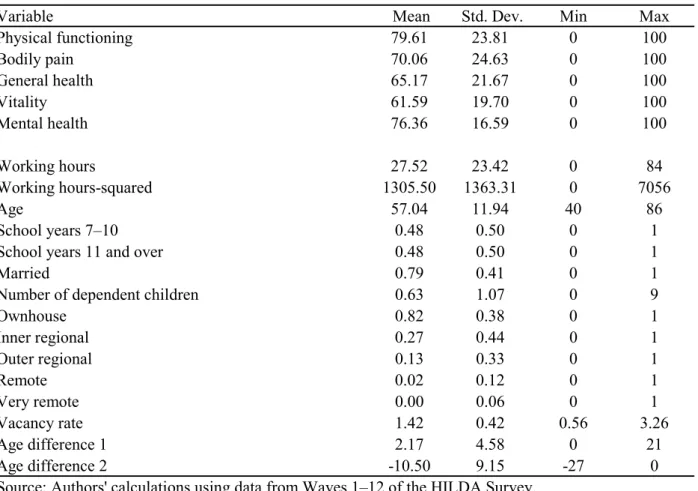
material indicates the effect of these criterion on the sample size available in each wave. Table II displays descriptive statistics on all the variables used in the analysis. In this table, Working hours is the respondent’s usual hours of working per week. As a result, the mean value of Working hours for males is 27.52 hours.
[Table II around here] 5. Estimation results
All regression results reported in this section are estimated using STATA version 15 (StataCorp, 2017).
5.1 Estimation using a fixed effect instrumental variable (FEIV) estimator
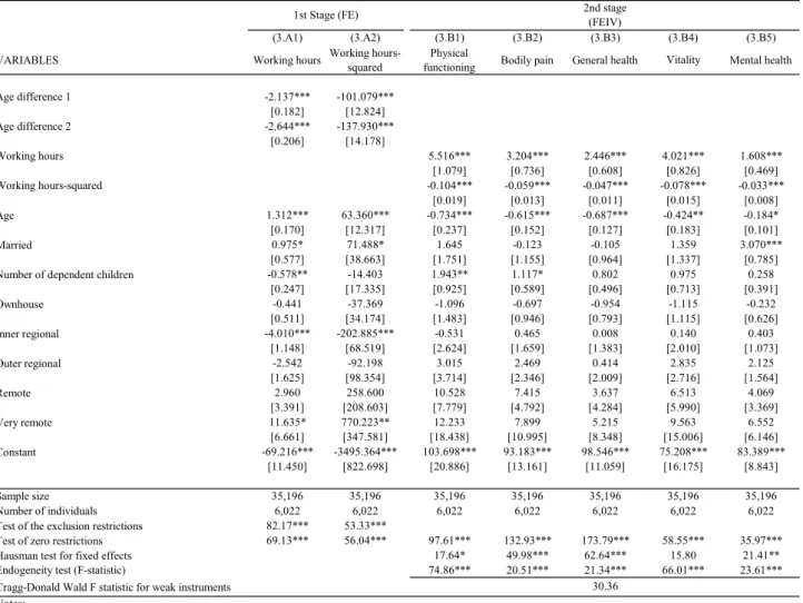
Table III presents the estimates for the equations in both the first and second stages of the fixed effect instrumental variable (FEIV) estimator. In stage 2 (columns (3.B1)–(3.B5)), where the fixed effect instrumental variable estimates of equation (1) are presented, it is observed that for each health variable both working hours and its square are individually statistically significant with the estimated coefficients have signs that are consistent with the a priori expectations suggested in section 3, so that there is an inverted U shape relationship between health and working hours. An examination of the endogeneity tests in Table III which test the joint significance of two residuals added to the model estimated by FE (see Wooldridge 2010, pp. 352–354), the results clearly reject the null hypothesis that Working hours and Working hours squared are exogenously determined. The Cragg-Donald (1993) test indicates we do not have a problem of “weak” instruments. Finally, the Hausman (1978) tests for choosing between the pooled IV model and FEIV indicate clearly that the FEIV estimator is to be preferred. In stage 1 (columns (3.A1)–(3.A2)) estimates of the “reduced form” equations for working hours (equation (2)) and workings hours squared (equation (3)) are displayed. The key variables, Age difference 1 and Age difference 2, are both individually and jointly significant in explaining the variation in working hours and working hours squared.
[Table III around here]
The results in Table III indicate that, for all health measures for males as working hours increase from zero the magnitude of the positive impact of working hours on their health status is decreasing until working hours reaches a threshold. Above the threshold, further increases in working hours have a negative impact on their self-assessed health status.
Where does the threshold occur? In other words, when does the impact of working hours on health status change from being positive to negative? The peaks occur around 26 hours for physical functioning, 27 hours for role physical, 26 hours for general health, 26 hours for
13
vitality, and 24 hours for mental health10. These are all slightly higher than the estimated
working hours (22–30 hours) for when cognitive abilities peak that are reported in Kajitani et al. (2017b).
In Figure II, we graph the relationship between impacts of working hours and self-assessed health status after controlling for other variables, using the estimated coefficients presented in Table III. Moreover, Figure II also shows that the health status of those working extremely long hours can be lower than those who are not working at all. This suggests that long working hours can lead to a deterioration of health status across the board for men.
[Figure II around here]
The results presented in Table III and graphed in Figure II show that there is non-linearity in the causal effects of working hours on self-assessed health status for middle aged and older males living in Australia. Our findings are consistent with our hypothesis, that is, work can help in maintaining health status for middle age and elderly male workers, but long working hours have a negative effect. Our results indicate that part-time work is an effective way to maintain to health in retirement.
5.2 Robustness Checks
Four robustness checks of the results in section 5.1 are presented here. They involve using a different estimator, using an additional instrumental variable, excluding full-time workers, and restricting the age of respondents. All these checks provide results that are consistent with the results in Table III.
The first robustness check involves an alternative way to generate some instruments by assuming the following equation to explain an individual’s hours worked:
𝑊𝐻∗ = 𝛾 𝐴𝑔𝑒 𝑑𝑖𝑓𝑓𝑒𝑟𝑒𝑛𝑐𝑒 1 + 𝛾 𝐴𝑔𝑒 𝑑𝑖𝑓𝑓𝑒𝑟𝑒𝑛𝑐𝑒 2 + 𝑋2 𝛿 + 𝑒 (4a)
𝑊𝐻 = 0 if 𝑊𝐻∗ ≤ 0
= 𝑊𝐻∗ if 0 < 𝑊𝐻∗, (4b)
where 𝑊𝐻∗ denotes an unobserved latent variable, which is connected to the observed
working hours 𝑊𝐻 through equation (4b). 𝑋2 consists of the same vector of control variables as used in equation (1a) and two control variables related to the level of schooling, and 𝑒 is a disturbance which is assumed to be normally, independently and identically
10 The 95% confidence intervals for these thresholds computed using bootstrapped estimates
of the standard errors based on 500 repetitions are: (24.8, 28.2) (Physical functioning), (25.2, 29.1) (Bodily pain), (24.1, 28.4) (General health), (24.1, 27.7) (Vitality) and (21.3, 26.5) (Mental health).
14 distributed with a zero mean and variance 𝜎 .
As is clear from equations (4a) and (4b), we have another issue in examining the effects of working hours on health, that is, working hours are censored (for example, retirees report zero working hours), so we estimate equations (4a) and (4b) using a Tobit estimator11. From
equations (4a) and (4b), the conditional expectation of 𝑊𝐻 can be computed as 𝐸(𝑊𝐻 |𝑍 ) = Φ 𝑍 𝜀
𝜎 𝑍 𝜀 + 𝜎𝜙 𝑍 𝜀
𝜎 (5),
where 𝑍 and 𝜀 are the vectors of regressors and parameters in equation (2), respectively, and Φ(∙) and 𝜙(∙) are the cumulative distribution function and probability distribution function of the standard normal distribution, respectively (see Greene 2008, p. 871). Using estimates of the parameters of equation (4a), this conditional expectation can be estimated. This estimate is denoted by 𝑊𝐻 . In estimating equation (1a) using a 2SLS procedure, 𝑊𝐻 and 𝑊𝐻 are then used as instruments for 𝑊𝐻 and 𝑊𝐻 , respectively (see Wooldridge 2010, p. 268). This estimator is labelled as Tobit+FEIV estimator. Zhang (2013) and Chi and Drewianka (2014) provide examples of this type of estimator in different contexts as a way to avoid the “forbidden regression” problem.
The results for this Tobit+FEIV estimator are reported in Table IV. The second stage estimates of equation (1a) for the five health variables are reported in columns (4.C1)–(4.C5). The results are similar to the results reported in Table III. The Tobit estimates of equations (4a) and (4b) are reported in column (4.A1) where we see that both the key variables, Age difference 1 and Age difference 2, are both individually and jointly significant in explaining the variation in working hours. The first stage of the FEIV estimates for Working hours and Working hours squared are reported in columns (4.B1) and (4.B2), respectively, and it can be seen that 𝑊𝐻 and 𝑊𝐻 are individually significant. It should be noted that because 𝑊𝐻 and 𝑊𝐻 are non-linear functions of 𝑍 the conditions that 𝑍 is required to satisfy for this estimator to be consistent are stronger than an instrumental estimator using just 𝑍 , so it is possible to compare these two estimators using a Hausman (1978) style testing procedure. This Hausman test is reported as Hausman test of three-stage estimator vs two-stage estimator, and indicates for three of the five health scores that the three-stage estimator is problematic compared to the two stage estimator reported in section 5.1. For this reason, the remaining results in this paper adopt the estimator use to generate the results in
11 Since we are estimating this model on panel data, it could be argued that we should employ
a Tobit estimator with fixed effects. Given the incidental parameter problem, this estimator would not provide a consistent estimator of any of the parameters of the model (see Greene, 2004), so we employ a pooled Tobit estimator.
15 Table III.
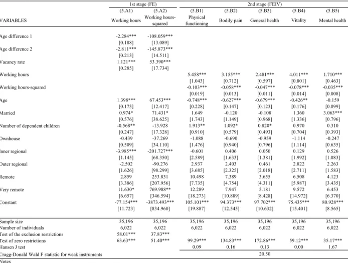
The results of the second robust check are reported in Table V reports where in addition to Age difference 1 and Age difference 2 the vacancy rate is also used as an instrument when estimating equation (1a) by FEIV. The vacancy rate shows both geographical (differing across each state) and temporal variation, and since it provides a measure of macroeconomic conditions at the state level is likely to affect the hours worked. On the other hand, it is unlikely to directly affect any of the health scores of individuals and so it is an appropriate instrument. As can be seen in columns (5.B1)–(5.B5), Working hours and Working hours squared are individually highly significant in all the equations and have estimated coefficients with the expected signs. All five health score equations pass the overidentifying test. In the first stage (columns (5.A1)–(5.A2)), the vacancy rate is highly significant in both equations.
The third robustness check restricts the analysis to exclude full-time workers. One potential criticism of our approach is that not all workers are free to choose their hours of work, so that it is inappropriate to treat hours worked as being endogenous for all workers. For example, in the absence of a collective agreement or award for full-time workers the ordinary hours of hours per week that they work is set at 38 hours12. In addition, full-time
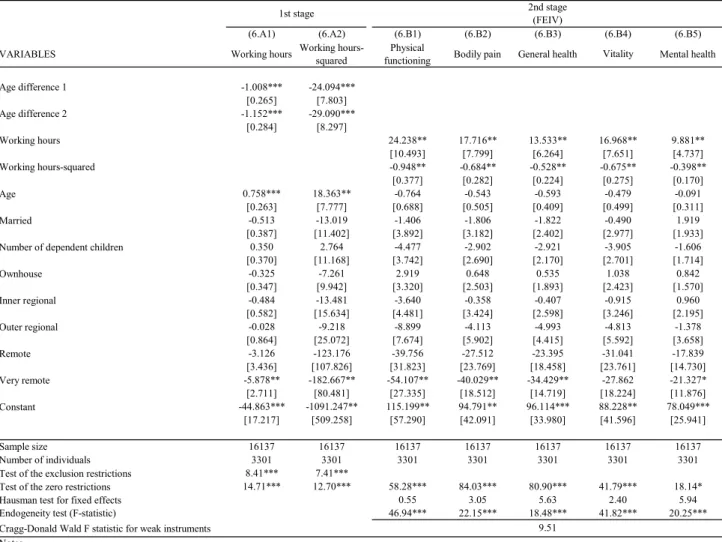
employees have the right to refuse to work unreasonable additional hours above this minimum number of bours worked. To take account of this possibility Table VI replicates Table III but excludes full-time workers. As a result of excluding full-time workers, the sample size is reduced from 35,196 to 16,137, and the number of individuals is reduced from 6,022 to 3,301. The results in Table VI are entirely consistent with the results obtained in Table III.
The final robustness test displayed in Table VII restricts the ages of respondents to the range 45–75. This reduces the sample from 35,196 to 25,865, and the number of individuals is reduced from 6,022 to 4,471. Excluding men aged over 75 years is likely to exclude people who have already stopped working due to retirement and whose average health status is lower than the rest of the sample. Individuals aged 40–44 in 2001 are more than 20 years away from their pension eligibility age, so that changes in their pension eligibility age may have little impact on their working hours. The results in Table VII are again consistent with the results in Table III, so that making these exclusions do not undermine our results.
5.3 Testing the Identifying Assumptions
12 Section 20 of the federal Fair Work Act of 2009. Available from URL:
https://www.legislation.gov.au/Details/C2018C00512 (Accessed 21 December 2019). Its predecessor, the federal Workplace Relations Act of 1996, contained a similar provision.
16
The final robustness check seeks to check some of the identifying assumptions underlying the analysis13. Given the non-linearities in (1a) and, we cannot write down an
explicit reduced form for 𝑦 . If we assume 𝛼 = 0 and make the structural equation in (1a) linear in working hours, then the reduced form is14
𝑦 = 𝜆 𝐴𝑔𝑒 𝑑𝑖𝑓𝑓𝑒𝑟𝑒𝑛𝑐𝑒 1 + 𝜆 𝐴𝑔𝑒 𝑑𝑖𝑓𝑓𝑒𝑟𝑒𝑛𝑐𝑒 2 + 𝑋1 𝜆 + 𝑣 , (6) Table VIII presents estimates of equation (6) for the five health measures estimated using all the data and a fixed effects (FE) estimator. In four of the five equations, 𝐴𝑔𝑒 𝑑𝑖𝑓𝑓𝑒𝑟𝑒𝑛𝑐𝑒 1 is statistically significant and in the other equation for mental health 𝐴𝑔𝑒 𝑑𝑖𝑓𝑓𝑒𝑟𝑒𝑛𝑐𝑒 2 is significant.
[Table VIII around here]
As can be seen from Table I, the pension eligibility age for individuals born on or before 30 June 1952 (hereafter called the 1951 “cohort”) does not change with the 2009 reform. If we imagine the reduced form age-health profiles prior to the 2009 pension reform, then in the analysis in section 5.1 for the 1951 cohort whose pension eligibility age does not change before and after the 2009 pension reform it is implicitly assumed that when they are under the age of 65 that their age-health profiles do not change around the time of the pension reform. Based on equation (6), we test this assumption using the following model estimated using data from Waves 1–12 for those individuals in the 1951 cohort who are not yet 6515:
13 We are greatly indebted to Daiji Kawaguchi for suggesting robustness tests along these
lines.
14 For women in the United Kingdom, Carrino et al. (2018) present estimates of the impact
of pension reform on health outcomes using a similar type of reduced form model.
15 Although equation (6) contains three age related variables, 𝐴𝑔𝑒 𝑑𝑖𝑓𝑓𝑒𝑟𝑒𝑛𝑐𝑒 1 ,
𝐴𝑔𝑒 𝑑𝑖𝑓𝑓𝑒𝑟𝑒𝑛𝑐𝑒 2 , and 𝐴𝑔𝑒 , so for a general test of structural change we would have the variables 𝐴𝑔𝑒 𝑑𝑖𝑓𝑓𝑒𝑟𝑒𝑛𝑐𝑒 1 , 𝐴𝑔𝑒 𝑑𝑖𝑓𝑓𝑒𝑟𝑒𝑛𝑐𝑒 2 , 𝐴𝑔𝑒 , 𝐴𝑔𝑒 𝑑𝑖𝑓𝑓𝑒𝑟𝑒𝑛𝑐𝑒 1 𝐴𝑓𝑡𝑒𝑟𝑅𝑒𝑓𝑜𝑟𝑚 , 𝐴𝑔𝑒 𝑑𝑖𝑓𝑓𝑒𝑟𝑒𝑛𝑐𝑒 2 𝐴𝑓𝑡𝑒𝑟𝑅𝑒𝑓𝑜𝑟𝑚 , 𝐴𝑔𝑒 𝐴𝑓𝑡𝑒𝑟𝑅𝑒𝑓𝑜𝑟𝑚 and 𝐴𝑓𝑡𝑒𝑟𝑅𝑒𝑓𝑜𝑟𝑚 . When the sample is limited to the 1951 cohort which has a constant pension eligibility age of 65, 𝐴𝑔𝑒 𝑑𝑖𝑓𝑓𝑒𝑟𝑒𝑛𝑐𝑒 1 + 𝐴𝑔𝑒 𝑑𝑖𝑓𝑓𝑒𝑟𝑒𝑛𝑐𝑒 2 = 𝐴𝑔𝑒 − 65 for all observations, so perfect multicollinearity exists among these three variables. This justifies dropping 𝐴𝑔𝑒 𝑑𝑖𝑓𝑓𝑒𝑟𝑒𝑛𝑐𝑒 1 , and 𝐴𝑔𝑒 𝑑𝑖𝑓𝑓𝑒𝑟𝑒𝑛𝑐𝑒 1 𝐴𝑓𝑡𝑒𝑟𝑅𝑒𝑓𝑜𝑟𝑚 . Similarly when the sample is limited to those members of the 1951 Cohort aged under 65 then 𝐴𝑔𝑒 𝑑𝑖𝑓𝑓𝑒𝑟𝑒𝑛𝑐𝑒 2 = 𝐴𝑔𝑒 − 65 , and 𝐴𝑔𝑒 𝑑𝑖𝑓𝑓𝑒𝑟𝑒𝑛𝑐𝑒 1 =0 for all observations, so we can only include one of these three variables; 𝐴𝑓𝑡𝑒𝑟𝑅𝑒𝑓𝑜𝑟𝑚 , 𝐴𝑔𝑒 𝑑𝑖𝑓𝑓𝑒𝑟𝑒𝑛𝑐𝑒 2 𝐴𝑓𝑡𝑒𝑟𝑅𝑒𝑓𝑜𝑟𝑚 and 𝐴𝑔𝑒 .
17
𝑦 = 𝜂 𝐴𝑓𝑡𝑒𝑟𝑅𝑒𝑓𝑜𝑟𝑚 + 𝜂 𝐴𝑔𝑒 𝑑𝑖𝑓𝑓𝑒𝑟𝑒𝑛𝑐𝑒 2 𝐴𝑓𝑡𝑒𝑟𝑅𝑒𝑓𝑜𝑟𝑚 + 𝑋1 𝜆 + 𝑣 , (7)
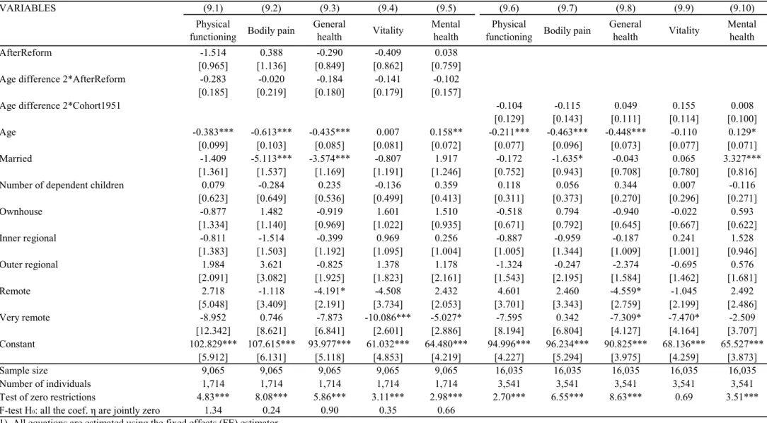
where 𝐴𝑓𝑡𝑒𝑟𝑅𝑒𝑓𝑜𝑟𝑚 is a 0–1 dummy variable taking the value 1 if the observation is after the pension reform of 2009, and 0 if the observation is before the pension reform of 2009. Equations (9.1)–(9.5) in Table IX present estimates of equation (7) estimated using a fixed effect (FE) estimator. It is easy to observe that the coefficients 𝜂 and 𝜂 are individually and jointly insignificant. That is, the pension reform has not affected the age-health profiles for individuals in the 1951 cohort who have not reached the age of 65.
[Table IX around here]
As can be seen from Table I, prior to the pension reform of 2009 the pension eligibility age for individuals in the 1951 cohort and for individuals born on or after 1 July 1952 (hereafter called the 1952 “cohort”) are the same. If we imagine the reduced form age-health profiles for these two groups of individuals aged under 65 prior to the 2009 pension reform, we are implicitly assuming them to be the same. Based on equation (6), we test this assumption using the following model estimated using data from Waves 1–8 for those individuals in the 1951 and the 1952 cohorts who have not reached the age of 6516:
𝑦 = 𝛿 𝐴𝑔𝑒𝑑𝑖𝑓𝑓𝑒𝑟𝑒𝑛𝑐𝑒 2 𝐶𝑜ℎ𝑜𝑟𝑡1951 + 𝑋1 𝜆 + 𝑣 , (8) where 𝐶𝑜ℎ𝑜𝑟𝑡1951 is a 0–1 dummy variable taking the value 1 if the individual is in the 1951 cohort, and taking the value zero if the individual is in the 1952 cohort. Equations (9.6) –(9.10) in Table IX presents FE estimates of (8) using individuals in the 1951 cohort who are under 65, and for individuals in the 1952 cohort using only data from before the 2009 reform. In no case is the parameter δ1 significantly different from zero supporting the assumption that
before the 2009 reform the 1951 and 1952 cohorts are similar. [Table IX around here]
16 Although equation (6) contains three age related variables, 𝐴𝑔𝑒 𝑑𝑖𝑓𝑓𝑒𝑟𝑒𝑛𝑐𝑒 1 ,
𝐴𝑔𝑒 𝑑𝑖𝑓𝑓𝑒𝑟𝑒𝑛𝑐𝑒 2 , and 𝐴𝑔𝑒 , so for a general test of structural change we would have the variables 𝐴𝑔𝑒 𝑑𝑖𝑓𝑓𝑒𝑟𝑒𝑛𝑐𝑒 1 , 𝐴𝑔𝑒 𝑑𝑖𝑓𝑓𝑒𝑟𝑒𝑛𝑐𝑒 2 , 𝐴𝑔𝑒 , 𝐴𝑔𝑒 𝑑𝑖𝑓𝑓𝑒𝑟𝑒𝑛𝑐𝑒 1 𝐶𝑜ℎ𝑜𝑟𝑡1951 , 𝐴𝑔𝑒 𝑑𝑖𝑓𝑓𝑒𝑟𝑒𝑛𝑐𝑒 2 𝐶𝑜ℎ𝑜𝑟𝑡1951 , 𝐴𝑔𝑒 𝐶𝑜ℎ𝑜𝑟𝑡1951 and 𝐶𝑜ℎ𝑜𝑟𝑡1951 . When the sample is limited to the pre-reform sample where all individuals have a constant pension eligibility age of 65 and individuals are assumed to be younger than 65, 𝐴𝑔𝑒 𝑑𝑖𝑓𝑓𝑒𝑟𝑒𝑛𝑐𝑒 1 + 𝐴𝑔𝑒 𝑑𝑖𝑓𝑓𝑒𝑟𝑒𝑛𝑐𝑒 2 = 𝐴𝑔𝑒 − 65, and 𝐴𝑔𝑒 𝑑𝑖𝑓𝑓𝑒𝑟𝑒𝑛𝑐𝑒 1 =0 for all observations. This justifies dropping 𝐴𝑔𝑒 𝑑𝑖𝑓𝑓𝑒𝑟𝑒𝑛𝑐𝑒 1 , 𝐴𝑔𝑒 𝑑𝑖𝑓𝑓𝑒𝑟𝑒𝑛𝑐𝑒 1 𝐶𝑜ℎ𝑜𝑟𝑡1951 , 𝐴𝑔𝑒 𝐶𝑜ℎ𝑜𝑟𝑡1951 and 𝐴𝑔𝑒 𝑑𝑖𝑓𝑓𝑒𝑟𝑒𝑛𝑐𝑒 2 . In addition, since 𝐶𝑜ℎ𝑜𝑟𝑡1951 is a time-independent variable and we are using a fixed effect estimator, its coefficient is not identified.
18 6. Concluding remarks
We examine the causal impact of working hours on the self-assessed health status of middle-aged and elderly males living in Australia using longitudinal data from the Household Income and Labour Dynamics in Australia (HILDA) Survey. The literature in this area is very limited in that it does not consider a non-linearity in the effect of working hours on health. Many previous studies examine the ‘use it or lose it’ hypothesis which tests whether or not retirement (not using your brain) leads to losses of cognitive functioning. On the other hand, we also examine the relevance of this hypothesis for a broader set of health outcomes. In addition, we focus on the ‘use it too much and lose everything’ hypothesis which refers to the situation where working too much can lead to not just a loss of cognitive functioning (see Kajitani et al. 2017b), but also declines in health status across the board. This study is unique in that we focus on not only labor market participation (the extensive margin), but also the intensive margin of work (working hours) and that we determine the optimal working hours for middle aged and elderly male workers in terms of maximizing their health status.
Using five measures of self-assessed health status in the SF-36, it is found that for working hours up to 24–27 hours per week increases in working hours have a positive impact on cognition for males depending on the health measure. After that, working hours have a negative impact on health status. Compared to males who do not work, working hours over 48–54 hours will lead to worse health outcomes depending on the measure. This indicates that the differences in working hours is an important factor in explaining differences in the health outcomes of middle aged and elderly male adults.
Thus, in middle and old age, adopting part-time work as a pattern of work could be effective in maintaining/improving the health status of individuals compared to when they do not work. Previous studies on retirement and cognitive functioning indicate that increasing the qualifying age for a pension can not only reduce the government social security expenditures but can potentially reduce the risk of cognitive deterioration. However, our study highlights that raising the qualifying age for a pension can reduce the risk of health deterioration, but that too much work can have quite adverse effects on health status.
Two important areas for future research are whether these results reported here for Australian males can be found for females and workers in other countries.
[Appendix I around here] Online Supplementary Material
19 References
Atalay K, Barrett GF. 2015. The impact of age pension eligibility age on retirement and program dependence: Evidence from an Australian experiment. Review of Economics and Statistics 97(1), 71–87. DOI: 10.1162/REST_a_00443
Atalay K, Barrett, GF, Staneva A. 2019. The effect of retirement on elderly cognitive functioning. Journal of Health Economics, 66, 37–53. DOI: 10.1016/j.jhealeco.2019.04.006
Australian Bureau of Statistics (ABS) (2011). &530.0 - Household Expenditure Survey, Australia: Summary of Results, 2009-10.9 September 2011. Accessed 26 September
2019. Available from URL:
https://www.abs.gov.au/ausstats/[email protected]/featurearticlesbyCatalogue/82CB91B5230 27894CA25790200154C25?OpenDocument
Bannai A, Tamakoshi A. 2014. The association between long working hours and health: A systematic review of epidemiological evidence. Scandinavian Journal of Work, Environment and Health 40(1), 5–18. DOI:10.5271/sjweh.3388
Bannai A, Ukawa S, Tamakoshi A. 2015. Long working hours and psychological distress among school teachers in Japan. Journal of Occupational Health 57(1), 20–27. DOI: 10.1539/joh.14-0127-OA
Barnay T. 2016. Health, work and working conditions: A review of the European economic literature. European Journal of Health Economics 17, 693–709. DOI: 10.1007/s10198-015-0715-8
Bassanini A, Caroli E. 2015. Is work bad for health? The role of constraint vs. choice. Annals of Economics and Statistics 119–120, 13–37. DOI: 10.15609/annaeconstat2009.119-120.13
Blake H, Garrouste C. 2017. Collateral effects of a pension reform in France. Accessed 10 December 2019. Available from URL: https://hal.archives-ouvertes.fr/hal-01500683/ Bonsang E, Adam S, Perelman S. 2012. Does retirement affect cognitive functioning?
Journal of Health Economics 31(3), 490–501. DOI: 10.1016/j.jhealeco.2012.03.005 Cai L, Kalb G. 2006. Health status and labour force participation: Evidence from Australia.
Health Economics 15, 241–261. DOI: 10.1002/hec.1053
Carrino L., Glaser K. & Avendano M. (2018). Later pension, poorer health? Evidence from the new state pension in the UK. Harvard Center for Population and Development Studies Working Paper. DOI: 10.2139/ssrn.3195760
Chi M, Drewianka S. (2014). How much is a green card worth? Evidence from Mexican men who marry women born in the U.S. Labour Economics, 31, 103–116. DOI:10.1016/j.labeco.2014.10.004
Coe NB, Zamarro G. 2011. Retirement effects on health in Europe. Journal of Health Economics 30(1), 77–86. DOI: 10.1016/j.jhealeco.2010.11.002
Collewet M, Sauermann J. 2017 Working hours and productivity. Labour Economics 47(1), 96–106. DOI:10.1016/j.labeco.2017.03.006
20
December 2016. Available from URL: http://www.budget.gov.au/2009-10/content/glossy/pension/download/pensions_overview.pdf#search='Securable+and +sustainable+pensions'
Cragg JG, Donald SG. 1993. Testing identifiability and specification in instrumental variable models. Econometric Theory 9(2), 222–240. DOI: 10.1017/S0266466600007519 De Grip A, Lindeboom M, Montizaan R. 2012. Shattered dreams: The effects of changing
the pension system late in the game. Economic Journal 122(559), 1–25. DOI: 10.1111/j.1468-0297.2011.02486.x
Frijters P, Johnston D, Meng X. 2009. The mental health cost of long working hours: The case of rural Chinese migrants. mimeo.
Greene W. 2004. The behavior of the maximum likelihood estimator of limited dependent variable models in the presence of fixed effects. Econometrics Journal 7(1), 98–119. DOI: 10.1111/j.1368-423X.2004.00123.x
Greene WH. 2008. Econometric Analysis, 6th edition. Pearson: New Jersey.
Hammer J. (2008). Pension Review. Background Paper. Accessed 25 September 2019.
Available from URL:
https://www.dss.gov.au/sites/default/files/documents/06_2012/pension_review_paper. pdf
Hausman JA. (1978). Specification tests in econometrics. Econometrica 46(6), 1251– 1271.DOI: 10.2307/1913827
Heller-Sahlgren G. 2017. Retirement blues. Journal of Health Economics 54(1), 66–78. DOI: 10.1016/j.jhealeco.2017.03.007
Kajitani S, Sakata K, McKenzie C. 2017a. Occupation, retirement and cognitive functioning. Ageing & Society 37(8), 1568–1596. DOI: 10.1017/S0144686X16000465
Kajitani S, McKenzie C, Sakata K. 2017b. Use it too much and lose it? The effect of working hours on cognitive ability, Panel Data Research Center at Keio University Discussion Paper no 2016-008.
Kudrna G, Woodland AD. 2011a. Implications of the 2009 age pension reform in Australia: A dynamic general equilibrium analysis. Economic Record 87, 183–201. DOI: 10.1111/j.1475-4932.2010.00703.x
Kudrna G, Woodland A. 2011b. An inter-temporal general equilibrium analysis of the Australian age pension means test. Journal of Macroeconomics 33(1), 61–79. DOI: 10.1016/j.jmacro.2010.09.006
Lee J, Lee YK. 2016. Can working hour reduction save workers? Labour Economics 40, 25– 36. DOI: 10.1016/j.labeco.2016.02.004
Llena-Nozal A. 2009. The effect of work status and working conditions on mental health in four OECD countries. National Institute Economic Review 209(1), 72–87. DOI: 10.1177/0027950109345234
21
Llena-Nozal A, Lindeboom M, Portrait F. 2004. The effect of work on mental health: Does occupation matter? Health Economics 13, 1045–1062. DOI: 10.1002/hec.929
Mazzonna F, Peracchi F. 2012. Ageing, cognitive abilities and retirement. European Economic Review 56(4), 691–710. DOI: 10.1016/j.euroecorev.2012.03.004
Mazzonna F, Peracchi F. 2017. Unhealthy retirement? Journal of Human Resources 52(1), 128–151. DOI:10.3368/jhr.52.1.0914-6627R1
Neumark D, Powers E. 2000. Welfare for the elderly: The effects of SSI on pre-retirement labor supply. Journal of Public Economics 78(1-2), 51–80. DOI: 10.1016/S0047-2727(99)00111-5
Neumark D, Powers E. 2003/2004.The effect of the SSI program on labor supply: Improved evidence from social security administrative files. Social Security Bulletin 65(3), 45– 60.
Neumark D, Powers E. 2005. The effects of changes in state SSI supplements on preretirement labor supply. Public Finance Review 33(1), 3–35. DOI: 10.1177/1091142104270655
Neumark D, Powers E. 2006. Supplemental security income, labor supply, and migration. Journal of Population Economic 19(3), 447–479. DOI: 10.1007/s00148-006-0074-y Nie P, Otterbach S, Sousa-Poza A. 2015. Long hours and health in China. China Economics
Review 33, 212–229. DOI: 10.1016/j.chieco.2015.02.004
Pencavel J. 2014. The productivity of working hours. Economic Journal 125, 2052–2076. DOI: 10.111/ecoj.12166
Pencavel J. 2016. Recovery from work and the productivity of working hours. Economica 83, 545–563. DOI: 10.1111/ecca.12206
Robone S, Jones A, Rice N. 2011. Contractual conditions, working conditions and their impact on health and well-being. European Journal of Health Economics 12(5), 429– 444. DOI: 10.1007/s10198-010-0256-0
Rohwedder S, Willis RJ. 2010. Mental retirement. Journal of Economic Perspectives 24(1), 119–138. DOI: 10.1257/089533010797456247
Schmitz H. 2011. Why are the unemployed in worse health? The causal effect of unemployment on health. Labour Economics 18(1), 71–79. DOI: 10.1016/j.labeco.2010.08.005
Sparks K, Cooper C, Fried Y, Shimon A. 1997. The effects of hours of work on health: A meta-analytic review. Journal of Occupational and Organizational Psychology 70(4), 391–408.
Spurgeon A, Harrington JM, Cooper C. 1997. Health and safety problems associated with long working hours: A review of the current position. Occupational and Environmental Medicine 54(6), 367–375. DOI: 10.1136/oem.54.6.367
22
Vere JP. 2011. Social security and elderly labor supply: Evidence from the Health and Retirement Study. Labour Economics 18, 676–686.DOI: 10.1016/j.labeco.2011.02.001 Ware JD. 2000. SF-36 Health Survey Update, Spine 25(24), 3130–3139.
Watson N, Wooden M. 2013. Adding a top-up sample to the Household, Income and Labour Dynamics in Australia Survey. Australian Economic Review 46(4), 489–498.
DOI: 10.1111/1467-8462.12027
Wooden M, Freidin S, Watson N. 2002. The Household, Income and Labour Dynamics in Australia (HILDA) Survey: Wave 1. Australian Economic Review 35(3), 339–348. DOI: 10.1111/1467-8462.00252
Wooldridge J. 2010. Econometric Analysis of Cross Section and Panel Data, 2nd edition, The
MIT Press: Cambridge.
Zhang Y. (2013). Does private tutoring improve students’ National College Entrance Exam performance? A case study from Jinan, China. Economics of Education Review 32, 1– 28. DOI: 10.1016/j.econedurev.2012.09.008
Appendix I: Definitions of Variables
Name Definition
Physical functioning The SF-36 physical functioning score (0–100) Bodily pain The SF-36 bodily score (0–100)
General health The SF-36 general health score (0–100)
Vitality The SF-36 vitality score (0–100)
Mental health The SF-36 mental health score (0–100)
Working hours The number of usual or average working hours per week the respondent works. Working hours-squared (Working hours)2
Age Respondent's age in years at the time of the survey School years 7–10
(benchmark: the respondent's highest years of school completed are under 7)
0–1 dummy variable taking the value of unity if the respondent's highest years of school completed are between 7 and 10, and 0 otherwise.
School years 11 and over
(benchmark: the respondent's highest years of school completed are under 7)
0–1 dummy variable taking the value of unity if the respondent's highest years of school completed are 11 and over, and 0 otherwise.
Married 0–1 dummy variable taking the value of unity if the respondent is currently married, and 0 otherwise.
Number of dependent children The number of the respondents' children who reside with him/her and are either are aged under 15 years or are aged 16–24 years and are enrolled in full-time education. Ownhouse 0–1 dummy variable taking the value of unity if the respondent owns his/her own
house or is currently paying off a mortgage, and 0 otherwise.
Inner regional 0–1 dummy variable taking the value unity if the respondent lives in inner regional Australia, and 0 otherwise.
Outer regional 0–1 dummy variable taking the value unity if the respondent lives in outer regional Australia, and 0 otherwise.
Remote 0–1 dummy variable taking the value unity if the respondent lives in remote Australia, and 0 otherwise.
Very remote 0–1 dummy variable taking the value unity if the respondent lives in very remote Australia, and 0 otherwise.
Age difference 1 =(Respondent's age in years at the time of the survey)-(Aged pension eligibility age) if the respondent has reached Aged pension eligibility age at the time of the survey, =0 otherwise
Age difference 2 =(Respondent's age in years at the time of the survey)-(Aged pension eligibility age) if the respondent has not yet reached Aged pension eligibility age at the time of the survey, =0 otherwise
Vacancy rate (Job vacancy/Employed)*100, where Job vacancy denotes the number of job
vacancies in the state where the respondent lives in each waves which are reported by the Australian Bureau of Statistics (ABS), and Employed denotes the number of total employed persons in the relevant state in November at each waves which are reported by the ABS. Noted that we use the values for May 2008 because of a lack of values for November 2008.
AfterReform 0-1 dummy variable taking the value unity if the observation is after May 2009, and 0 otherwise.
Cohort1951 0-1 dummy variable taking the value unity if individual was born before or on 30 June 1952, and 0 otherwise.
Birthday (Age) Sample (%)
Wave 1 Wave 8 Wave 9
Up to 30 June 1952
(Aged 49 and older in Wave 1) 65 68.6% 50.8% 65 47.9%
1 July 1952 to 31 December 1953 (Aged 47–48 in Wave 1) 65 5.0% 3.8% 65.5 3.7% 1 January 1954 to 30 June 1955 (Aged 46 in Wave 1) 65 3.8% 2.5% 66 2.8% 1 July 1955 to 31 December 1956 (Aged 44–45 in Wave 1) 65 4.9% 3.8% 66.5 3.6% From 1 January 1957
(Aged 43 and younger in Wave 1) 65 17.7% 39.1% 67 42.0%
Total 100.0% 100.0% 100.0% Number of Observations 2,893 2,713 2,725 Sample (%) Pension eligibility age before April 2009 Pension eligibility age after
May 2009
Source: For pension eligibility ages: Commonwealth of Australia (2009), p. 9. Sample proportions in each group are authors' calculations using data from the HILDA Survey.
Table II: Descriptive Statistics
Variable Mean Std. Dev. Min Max
Physical functioning 79.61 23.81 0 100 Bodily pain 70.06 24.63 0 100 General health 65.17 21.67 0 100 Vitality 61.59 19.70 0 100 Mental health 76.36 16.59 0 100 Working hours 27.52 23.42 0 84 Working hours-squared 1305.50 1363.31 0 7056 Age 57.04 11.94 40 86 School years 7–10 0.48 0.50 0 1
School years 11 and over 0.48 0.50 0 1
Married 0.79 0.41 0 1
Number of dependent children 0.63 1.07 0 9
Ownhouse 0.82 0.38 0 1 Inner regional 0.27 0.44 0 1 Outer regional 0.13 0.33 0 1 Remote 0.02 0.12 0 1 Very remote 0.00 0.06 0 1 Vacancy rate 1.42 0.42 0.56 3.26 Age difference 1 2.17 4.58 0 21 Age difference 2 -10.50 9.15 -27 0
Source: Authors' calculations using data from Waves 1–12 of the HILDA Survey.
Note: 35,196 observations from 6,022 individuals are used to compute the descriptive statistics in each case.
Table III: The impacts of working hours on health
(3.A1) (3.A2) (3.B1) (3.B2) (3.B3) (3.B4) (3.B5) VARIABLES Working hours Working
hours-squared
Physical
functioning Bodily pain General health Vitality Mental health Age difference 1 -2.137*** -101.079*** [0.182] [12.824] Age difference 2 -2.644*** -137.930*** [0.206] [14.178] Working hours 5.516*** 3.204*** 2.446*** 4.021*** 1.608*** [1.079] [0.736] [0.608] [0.826] [0.469] Working hours-squared -0.104*** -0.059*** -0.047*** -0.078*** -0.033*** [0.019] [0.013] [0.011] [0.015] [0.008] Age 1.312*** 63.360*** -0.734*** -0.615*** -0.687*** -0.424** -0.184* [0.170] [12.317] [0.237] [0.152] [0.127] [0.183] [0.101] Married 0.975* 71.488* 1.645 -0.123 -0.105 1.359 3.070*** [0.577] [38.663] [1.751] [1.155] [0.964] [1.337] [0.785] Number of dependent children -0.578** -14.403 1.943** 1.117* 0.802 0.975 0.258
[0.247] [17.335] [0.925] [0.589] [0.496] [0.713] [0.391] Ownhouse -0.441 -37.369 -1.096 -0.697 -0.954 -1.115 -0.232 [0.511] [34.174] [1.483] [0.946] [0.793] [1.115] [0.626] Inner regional -4.010*** -202.885*** -0.531 0.465 0.008 0.140 0.403 [1.148] [68.519] [2.624] [1.659] [1.383] [2.010] [1.073] Outer regional -2.542 -92.198 3.015 2.469 0.414 2.835 2.125 [1.625] [98.354] [3.714] [2.346] [2.009] [2.716] [1.564] Remote 2.960 258.600 10.528 7.415 3.637 6.513 4.069 [3.391] [208.603] [7.779] [4.792] [4.284] [5.990] [3.369] Very remote 11.635* 770.223** 12.233 7.899 5.215 9.563 6.552 [6.661] [347.581] [18.438] [10.995] [8.348] [15.006] [6.146] Constant -69.216*** -3495.364*** 103.698*** 93.183*** 98.546*** 75.208*** 83.389*** [11.450] [822.698] [20.886] [13.161] [11.059] [16.175] [8.843] Sample size 35,196 35,196 35,196 35,196 35,196 35,196 35,196 Number of individuals 6,022 6,022 6,022 6,022 6,022 6,022 6,022 Test of the exclusion restrictions 82.17*** 53.33***
Test of zero restrictions 69.13*** 56.04*** 97.61*** 132.93*** 173.79*** 58.55*** 35.97*** Hausman test for fixed effects 17.64* 49.98*** 62.64*** 15.80 21.41** Endogeneity test (F-statistic) 74.86*** 20.51*** 21.34*** 66.01*** 23.61*** Cragg-Donald Wald F statistic for weak instruments
8) The Cragg-Donald Wald F statistic reported is computed using the "xtivreg2" command in STATA 15.
1st Stage (FE) 2nd stage(FEIV)
Notes:
2) *, ** and *** indicate statistical significance at the 10%, 5% and 1% levels, respectively.
4) Test of the exclusion restrictions reports an F-test for the null hypothesis that the coefficients on Age difference 1 and Age difference 2 are jointly zero. 30.36
1) The first stage equations have been estimated using an individual fixed effects (FE) estimator and the second stage equations have been estimated using an individual fixed effect instrumental variable (FEIV) estimator.
3) Figures reported in square brackets are robust standard errors adjusted for clustering.
7) The Endogeneity test tests the null hypothesis that Working hours and Working hours-squared in the second stage can be treated as being exogenous. Following Wooldridge (2010, pages 352–354), this test is implemented as an F-test that tests the joint significance of the residuals from the two first stage equations when added to each of the second stage models and these second stage models are estimated by a fixed effects estimator.
5) Test of zero restrictions reports a test of the null hypothesis that all the coefficients except the constant are jointly zero. This test is computed as an F-test in Stage 1 and a Wald test in Stage 2.
6) The Hausman test for fixed effects reports a Hausman test for the null pooled model estimated by instrumental variables against the fixed effect model estimated by instrumental variables. The test is based on 500 bootstrap repetitions using the "rhausman" command in STATA 15.