鳥取大学研究成果リポジトリ
Tottori University research result repository
タイトル
Title
Effects of Cage-Breaking Events in Single-File
Diffusion on Elongation Correlation
著者
Auther(s)
Ooshida, Takeshi; Otsuki, Michio
掲載誌・巻号・ページ
Citation
Journal of the Physical Society of Japan , 86 (11) :
113002 - 113002
刊行日
Issue Date
2017-10-24
資源タイプ
Resource Type
学術雑誌論文 / Journal Article
版区分
Resource Version
著者版 / Author
権利
Rights
© 2017 The Physical Society of Japan (J. Phys. Soc.
Jpn. 86, 113002.)
DOI
10.7566/JPSJ.86.113002
Typeset with jpsj3.cls<ver.1.1> Letter
Effects of Cage-Breaking Events in Single-File Diffusion on Elongation Correlation
Ooshida Takeshi1∗and Michio Otsuki2
1Department of Mechanical and Aerospace Engineering, Tottori University, Koyama, Tottori 680-8552, Japan 2Department of Materials Science, Shimane University, Matsue 690-8504, Japan
(Received 2017-08-28)
Collective motion of caged particles is studied by calculating correlations of elongations (i.e. ex-cess distances between two tagged particles) in a one-dimensional colloidal system, with the focus on the effect of overtaking events by which particles can hop out of the cage. It is shown analytically and verified numerically that the effect of overtaking is more prominent in shorter lengthscales, and also that the two-time elongation correlation exhibits ageing behavior due to overtaking.
KEYWORDS: single-file diffusion, overtaking, caged particles, collective motion, elongation correlation, Brownian dynamics, colloidal system, Rouse model, Lagrangian de-scription, label variable
Various soft materials have properties between the liquid-like and solid-like consistencies, asso-ciated with collective dynamics of the constituents. As one of the simplest cases of such materials, one may mention a single elastic chain with thermal fluctuation, namely the Rouse model.1, 2Indeed, the chain is not liquid nor solid in the usual sense: every monomer in the Rouse chain is inseparably bonded to its neighbors, yet its mean square displacement (MSD) can grow unlimitedly, in proportion to the square root of the elapsed time t.
The above-mentioned behavior of MSD ∝ √t is shared by one-dimensional (1D) systems of Brownian particles with repulsive interaction that disallows the particles to exchange their positions. This is known as the single-file diffusion (SFD).3–5In the ideal case in which the barrier height of the
interaction potential, Vmax, is infinitely large, every particle is eternally caged between its neighbors,
and the longtime dynamics are equivalent to those of the Rouse model.5, 6 The growth of MSD is
understood as a collective motion of particles comprising the cage, which is due to the dominance of long-wave fluctuations peculiar to low-dimensional systems and akin to the logarithmic behavior of the MSD in two-dimensional (2D) systems.7–9
More generally, collective motions in glassy dynamics of soft materials require four-point space-time correlations for their quantification.10, 11 Dynamical susceptibilityχ4 is one of such four-point
correlations, developed for computational ease, though its behavior is rather difficult to interpret, as signals from different processes are mixed in it.12–15Some other types of space-time correlations are
therefore needed. While the weakest point ofχ4 is that the effect of quasi-uniform cage drift appears
as a decaying factor which obscures the growth of correlation length, it is known that this weakness can be overcome by space-time correlations based on the idea of particle tracking. In numerical anal-ysis of glassy liquids, this idea has been implemented as bond breakage correlation,13, 16, 17which is completely frame-independent. Displacement correlation, which is also based on particle tracking, has the advantage of analytical tractability in some cases.5, 12, 14, 18, 19
Here we propose yet another space-time correlation, which at once inherits the strong points of the bond breakage correlation, being free from undesirable effect of drift, and allows analytical calculation in the same way as the displacement correlation. The idea is to target on correlations of elongation, analogous to the interparticle distance correlation previously studied by Lizana et al.6for ideal SFD on the basis of the elastic approximation (i.e. the Rouse model).
As an example to illustrate our calculation scheme of elongation correlation Cε, going beyond the elastic approximation, here we take SFD with overtaking,19–22 allowing the particles to hop out of the cage. Although there has been a number of studies on the crossover behavior of MSD (from √
t to t) in SFD with overtaking as a cage-breaking event, to the best of our knowledge, none of them have presented analytical calculation of space–time correlations to clarify the effect of overtaking on the collective motion. We establish a framework for analytical calculation of Cε, extending the label variable method.5, 14, 18, 19, 23As a result, within a certain approximation justifiable in the limit of rare
overtaking, Cεis obtained as a sum of two parts: a contribution from the density fluctuation in the chain of the caged particles, and the effect of overtaking. At larger lengthscales the former predominates, while the latter has an impact on the shortscale behavior of Cε.
The system is specified as follows: The position of the i-th particle, Xi = Xi(t), is subject to the
Langevin equation m ¨Xi = −µ ˙Xi− ∂ ∂Xi ∑ j<k V(Xk− Xj)+ µ fi(t), (1)
where m is the mass of the particle,µ is the drag coefficient (a scalar constant), and µ fi(t) is the random
force characterized by the free-particle diffusivity D = kBT/µ. The periodic boundary condition,
Xj+N = Xj+ L, implies the mean density ρ0= N/L. The interaction potential, determining the particle
diameter σ, is specified as V(±r) = Vmax(1− r/σ)2 for 0 ≤ r ≤ σ and V(r) = 0 otherwise; Vmaxis
large but finite, allowing neighboring particles to exchange their positions as a rare event.
On the basis of{Xi}i=1,2,...,N, we define the elongation of the particle pair (i, j) relative to the initial
configuration, as εi, j(t) def = Xj(t)− Xi(t) Xj(0)− Xi(0)− 1. (2)
J. Phys. Soc. Jpn. Letter
Its correlation, as a function of two time arguments s and t and the initial separation ˜d (, 0), is then introduced as
Cε( ˜d, t, s)def= ˜d2⟨εi, j(t)εi, j(s)
⟩
˜
d (0≤ s < t), (3)
where⟨ ⟩d˜denotes conditional thermal averaging over the pairs (i, j) such that Xj(0)− Xi(0)= ˜d.
For simplicity, here we limit the initial condition mainly to the equidistant configuration, Xi(0) =
X0(0)+ iℓ0 whereℓ0 def
= L/N = ρ−1
0 . In this case, Eq. (3) requires integer values of ˜d/ℓ0, which we
denote with∆ (= ˜d/ℓ0∈ Z), so that
εi,i+∆(t)=
Xi+∆(t)− Xi(t)
ℓ0∆ − 1.
(4) As long as it is not confusing, we will write simply Cε(∆, t, s) instead of Cε(ℓ0∆, t, s). A variant of Cε
for a single time is also introduced analogously: C0ε(∆, s)def= lim t→sCε(∆, t, s) = ℓ02∆2 N ∑ i ⟨[ε i,i+∆(s) ]2⟩. (5)
Theoretical approach to these statistical quantities is grounded on hydrodynamical field variables. The coarse-grained dynamics of {Xi}i=1,2,...,N for timescales greater than m/µ are described by the
Dean–Kawasaki equation,24, 25with the fluctuating density fieldρ and its flux Q defined as ρ = ρ(x, t) =∑ i ρi(x, t), Q = Q(x, t) = ∑ i ρi(x, t) ˙Xi(t),
whereρi(x, t) = δ(x − Xi(t)) is the single-body density.
Subsequently, we introduce the label variableξ to incorporate the idea of particle tracking into the continuum description.5, 14, 18, 19, 23 We define ξ = ξ(x, t) as a solution to the equation (ρ, Q) = (∂xξ, −∂tξ), so that ξ satisfies
ρ (∂t+ u ∂x)ξ(x, t) = 0, (6)
with u such that Q = ρu. The convective equation (6) implies that, if we define Ξi(t)
def
= ξ(Xi(t), t),
its value is basically independent of t. In the absence of overtaking,Ξi(t) is actually equivalent to the
numbering of the particle. The constancy ofΞi(t) is checked by calculating its t-derivative as23
dΞi(t) dt = ˙Xi(t) ∂ξ ∂x x=Xi + ∂ξ∂t x=Xi = (ρ ˙Xi− Q) x=Xi, (7) which should vanish unless some other particle, say the j-th one, overlaps the i-th particle. As a result of the overlap in exceptional cases,Ξi(t) changes its value if the velocity difference ˙Xi− ˙Xj, 0 persists
until the two particles exchange their positions: this is what we refer to as overtaking.
The overtaking event is thus formulated as a change in the values ofΞi(t) andΞj(t), such that their
values are exchanged: Ξi(t2) = Ξj(t1) andΞj(t2) = Ξi(t1), where t1 and t2 denote times before and
interpreted as a kind of local conservation law forΞi(t) describing a topological constraint.
Apart from the overtaking event that allows a particle to hop out of the cage, the dynamics of each caged particle in the present system are governed by collective motion of the surrounding particles. This collective motion is described through density fluctuations; it is useful to express it with
ψ = ψ(ξ, t)def= ℓ0−1
∂x
∂ξ − 1, (8)
and introduce the Fourier representation, defined as ψ(ξ, t) =∑
k
ˇ
ψ(k, t)e−ikξ, ψ(k, t) =ˇ ∫ eikξψ(ξ, t)dξ
N, (9)
where k/(2π/N) ∈ Z. The field ψ is governed by a transformed version of the Dean–Kawasaki equa-tion,5, 14, 18, 19, 23given as Eq. (2.12) in Ref. 14, whose linear approximation is found to be equivalent to the Rouse model1, 2, 5 and the 1D Edwards–Wilkinson equation.12, 26 Let us thereby calculate the elongation correlation Cε(∆, t, s), defining14, 23
Cψ(k, t, s)def= N L2
⟨ ˇ
ψ(k, t) ˇψ(−k, s)⟩. (10)
We begin with expressing x= x(ξ, t) as an indefinite integral of ∂x/∂ξ. Using Eqs. (8) and (9), we find x= x(ξ, t) = ℓ0ξ + ℓ0 ∑ k e−ikξψ(k, t)ˇ −ik + XG(t), (11)
where XG(t) is the center-of-mass fluctuation that vanishes for large systems.5Evaluation atξ = Ξj(t)
then yields Xj(t)= ℓ0Ξj(t)+ ℓ0 ∑ k e−ikΞj(t)ψ(k, t)ˇ −ik . (12)
From Eqs. (4) and (12), in principle, a formula to calculate Cεfrom Cψcan be derived. This derivation is carried out firstly in the case of the ideal SFD without overtaking, and secondly in the case in which overtaking is rare but not negligible.
In the first case, in whichΞj(t) is frozen to its initial valueΞj(0)= Ξ0j as overtaking is forbidden,
Eq. (4) reads εj, j+∆(t)= 1 ∆ ∑ k e−ikΞ0je −ik∆− 1 −ik ψ(k, t).ˇ (13)
Then we multiply Eq. (13) with its duplicate in which (k, t) is replaced with (−k′, s), and expand the double summation. Taking into account that the terms with k , k′ vanish on the average, we arrive at the formula in the absence of overtaking:
Cε(∆, t, s) = 2ℓ20∑ k 1− cos k∆ k2 ⟨ ˇ ψ(k, t) ˇψ(−k, s)⟩
J. Phys. Soc. Jpn. Letter → L4 πN2 ∫ +∞ −∞ 1− cos k∆ k2 Cψ(k, t, s)dk. (14)
This formula (14) allows us to express Cε more concretely, if a concrete expression for Cψ is available. Here we use5, 26
Cψ(k, t, s) = S L2e −Dc ∗k2(t−s)+Sinit− S L2 e −Dc ∗k2(t+s) (15)
with Dc∗ = ρ20D/S , obtained from the linearized equation for ψ, with the non-equilibrium initial con-dition taken into account; S denotes the long-wave limiting value of the static structure factor in the equilibrium state, and Sinitis the value corresponding to the initial condition (Sinit = 0 for the
equidis-tant configuration). The integral in Eq. (14) is then evaluated, which yields Cε(∆, t, s) Sℓ20∆ = φε ∆ 2√Dc∗(t− s) − φε ∆ 2√Dc∗(t+ s) , (16)
where the functionφε( · ) is defined as
φε(θ)def= erf θ +−1 + e −θ2 √π θ ≃ θ √ π − θ 3 6√π + · · · (|θ| ≪ 1) 1− √1 π θ (θ → +∞).
Notice the ageing effect in Eq. (16): if t − s is fixed, still Cεdepends on s. In particular, for t→ s we have
C0ε(∆, s) = S ℓ20∆[1− φε(θ0)], θ0 def= √∆
8Dc∗s, (17)
which is s-dependent (unless s ≫ ∆2/Dc∗). We also note that, if ageing is negligible (s ≫ ∆2/Dc∗and t− s ≪ s), Eq. (16) seems to be consistent with the result by Lizana et al.6
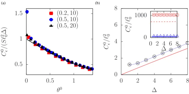
In Fig. 1, the values of C0ε predicted by Eq. (17) are compared with those computed directly from Eq. (1). Except for the choice of V(r) and the initial condition, the numerical calculation was performed in the same way as in Ref. 19, with finite inertia (m/µ : σ2/D = 1 : 1). The data in Fig. 1(a), plotted againstθ0, are seen to collapse onto a master curve given by Eq. (17), except for the systematic deviation at small values ofθ0. The case with the largestρ0and the smallest Vmax, namely
(ρ0, Vmax) = (0.5σ−1, 10kBT ), deviates most prominently. As this deviation is due to the omission of
overtaking, now we need to proceed to the second case.
Let us discuss how the formula (14) is modified by overtaking, restarting from Eq. (12). For the sake of brevity, we defineδΞj(t)
def
= Ξj(t)− Ξj(0)= Ξj(t)− Ξ0j. On the assumption of rare overtaking,
we regardδΞj(t) as a small perturbation, which allows linearizing Eq. (12) in ( ˇψ, δΞj) as
Xj(t)≃ ℓ0Ξ0j + ℓ0δΞj(t)+ ℓ0 ∑ k e−ikΞ0j ˇ ψ(k, t) −ik . (18)
(a) (b) ✵ ✿✺ ✶ ✶✿✺ ✵ ✵ ✿✺ ✶ ✵ ✷ ✹ ✻ ✽ ✵ ✷ ✹ ✻ ✽ ✵ ✶✵ ✵ ✵ ✵ ✷ ✹ ✻ ✽ ❈ ✎ ❂ ✭ ❙ ❵ ✁ ✂ ✮ ✒ ✄ ☎✵ ✿✷ ❀✶✵✆ ☎✵ ✿✺❀✶✵✆ ☎✵ ✿✺❀✷✵✆ ❈ ✎ ❂ ❵ ✁ ✝ ❈ ✎ ❂ ❵ ✁ ✝
Fig. 1. (Color online) Numerical values of C0
ε. (a) A plot againstθ0 = ∆/√8Dc∗s, rescaled with Sℓ20∆. Three
cases are included: (ρ0σ, βVmax)= (0.2, 10), (0.5, 10) and (0.5, 20). In each case, data are computed with
N = 500, recorded at s = 1000 σ2/D, and averaged over 480 runs for each plotted point. The solid line
represents the master curve predicted by Eq. (17). (b) A replot of C0
ε(∆, s)/ℓ20versus∆, for (ρ0σ, βVmax)=
(0.5, 10) and s = 4000 σ2/D, shown with circles (◦). The lines represent theoretical predictions: the solid
line represents Eq. (17), while the dotted line is given by Eq. (25) with H0 taken into account, where
να = 3.15 × 10⁻⁵D/σ2according to Eq. (22). Inset: an analogous plot withβV
max = 2 (broken line for the
theory and circles for numerical values) andβVmax= 5 (solid line and triangles).
Then, following the same line of argument as in the derivation of Eq. (14), we find Cε(∆, t, s) = 2ℓ02∑ k 1− cos k∆ k2 ⟨ ˇ ψ(k, t) ˇψ(−k, s)⟩+ ℓ2 0H(∆, t, s) (19) where H(∆, t, s)def = ⟨[δΞj(t)− δΞi(t) ] [ δΞj(s)− δΞi(s) ]⟩ j−i=∆.
The first term on the right-hand side of Eq. (19) reproduces Eq. (16), while the second term needs to be evaluated separately. To be consistent with the treatment ofψ based on the Dean–Kawasaki equa-tion, the overtaking process should be treated on the basis of Dean’s equation24 forρi(x, t). However,
within the approximation of the present analysis, a phenomenological modeling will suffice.
We model the overtaking as a random process in which a particle is exchanged with its neighbor at the frequencyνα, such that⟨[δΞj(t)− δΞj(s)]2
⟩
= 2να(t− s). Assuming that distinct exchanges are uncorrelated, we have
H(∆, t, s) = H(∆, s, s)def= H0(∆, s) (0 ≤ s < t). (20) This is further evaluated by calculating the pair distribution function for (δΞi(s), δΞi+∆(s)), as
H0(∆, s) = s + s e−s[I∆−1(s)+ I∆(s)]+ (−2∆ + 1)e−s
∞
∑
n=∆
J. Phys. Soc. Jpn. Letter
where s= 4ναs and Indenotes the modified Bessel function of the first kind. In particular, for∆ ≫ 1,
Eq. (21) can be approximated by the first term alone, i.e. H0(∆, s) ≃ 4ναs.
The overtaking frequencyναis given by an Arrenius-like expression, with a prefactor that depends on both the barrier hight Vmaxand the mean densityρ0. In the present system, numerical data ofνα
can be fitted by να = D ( a0ρ0 σ + a1ρ20βVmax ) e−βVmax, β = 1 kBT, (22) with a0≈ 1/2 and a1≈ 1/6.
The prediction by Eq. (19) is summarized as follows: Using the similarity variables θdef
= ∆
2√Dc∗(t− s), θ
′ def= ∆
2√Dc∗(t+ s) (23)
suggested by Eq. (16), we find Eq. (19) to predict
Cε(∆, t, s) = S ℓ02∆[φε(θ) − φε(θ′)]+ ℓ20H0(∆, s), (24) with the hopping term estimated by Eqs. (21) and (22). In the limit of t→ s, we also have
Cε0(∆, s) = S ℓ20∆[1− φε(θ0)]+ ℓ20H0(∆, s) (25) in place of Eq. (17). Let us test these predictions.
The prominent deviation from Eq. (17), seen in Fig. 1(a) for (ρ0, Vmax) = (0.5σ−1, 10kBT ), is
clarified on the basis of Eq. (25). The replot in Fig. 1(b) exhibits a nearly uniform deviation from Eq. (17), attributable to the last term in Eq. (25) and consistent with Eq. (21). Note, however, that quantitative agreement is lost if Vmaxis so low that frequent overtaking events invalidate the present
theory; see the Inset of Fig. 1(b).
The t-dependence of Cε = Cε(∆, t, s) predicted by Eq. (24) is verified in Fig. 2, where Cεis plotted against t− s. We have chosen a large value of s, so that φε(θ′) in Eq. (24) is negligible. In the case of Vmax = 20kBT , the barrier is so high that the hopping termℓ20H0(∆, s) is also negligible; this means
that Cεis given byφε(θ) alone, as is shown by the lower solid line in Fig. 2, and Cεdecays away for t− s → +∞. Contrastively, if the barrier is lower, Cεremains finite for t− s → +∞, as the hopping term contributes to it. We have evaluated limt−s→∞Cε(∆, t, s) by means of fitting, as is exemplified by
the dashed line in Fig. 2. The residual values thus obtained, denoted with C∞ε and normalized with ℓ2
0, are plotted against 4ναs in the inset of Fig. 2, withνα given by Eq. (22). The result seems to be
reasonably close to the theoretical prediction, C∞ε/ℓ20 ≃ 4ναs.
Thus we have presented a scheme to calculate Cε in SFD with overtaking, by expressing the motion of particles in terms of ˇψ(k, t) and δΞj(t). The field ˇψ(k, t) represents fluctuation of density
(a) (b) ✵ ✷ ✹ ✻ ✽ ✶✵ ✶✵ ✶✵ ✁ ✶✵ ✸ ✶✵ ✂ ✵ ✵✿✺ ✵ ✵✿✺ ❈ ✎ t✄s ❱ ♠❛① ❂ ✶✵❦ ❇ ❚ ❱ ♠❛① ❂ ✷ ✵❦ ❇ ❚ ❈ ☎ ✎ ✆ ❵ ✝ ✞ ✹✗ ☛ s
Fig. 2. (Color online) (a) Decay of Cε(∆, t, s) with regard to t. The two cases of Vmax = 10kBT and Vmax =
20kBT (withρ0 = 0.5σ−1 in common) are compared by plotting Cε against t− s, with s = 4000 σ2/D
and∆ = 3 fixed; 160 runs are averaged in each case. The solid lines represent theoretical curves predicted by Eq. (24), and the dashed line results from fitting with A+ B(t − s)−1/2. (b) Numerical values of C∞ε = limt−s→∞Cε(∆, t, s), nondimensionalized with ℓ20and plotted against 4ναs, i.e. the leading term in Eq. (21).
The squares, circles and triangles denote (ρ0σ, βVmax)= (0.5, 10), (0.5, 12) and (0.3, 10), respectively; the
filled symbols represent results for∆ = 3, and the open ones for ∆ = 5.
linear approximation, Cεis obtained in Eq. (24) as a sum of two contributions from ˇψ and δΞj. The
effect of overtaking is prominent at shorter lengthscales, but it has a relatively small impact on the long-range correlation (Fig. 1). This is naturally understood, on one hand, by considering that the overtaking process in SFD is a short-scale event involving only two neighboring particles explicitly. This interpretation suggests, on the other hand, that it will be quite intriguing to extend the present framework to systems in which cage-breaking events involve many particles, as the result will provide information about the space-time scales of such events.
The hopping term ℓ02H0(∆, s) in Eqs. (24) and (25) depends on s and grows unlimitedly. This means that Cεnever equilibrates: Cεis subject to an extra ageing effect due to overtaking, in addition to the effect of Sinit, S on Cψin Eq. (15). Besides, the temporal behavior of H0and Cψin the present
system are quite similar to that of the correlations of rotational and dilatational modes of deformation in 2D colloidal liquids.5, 18 On this analogy, we expect that more insight may be given by profound studies of overtaking: for example, theρ0-dependence ofνα in Eq. (22) may be clarified by ideas in
Ref. 22 and suggest an extension to 2D colloidal glasses.
In a wider context of glassy dynamics, cage-breaking events can be conceived as transition be-tween configurations corresponding to local basins of the energy landscape, often termed as inherent
J. Phys. Soc. Jpn. Letter
structures.27 The overtaking event in SFD is among the simplest examples of such transition. As is shown in Fig. 2, the effect of this transition between inherent structures remains in Cεfor t− s → ∞. In other words, the “natural distance” between the two tagged particles has changed from its initial value. This is reminiscent of the theory of elastoplasticity in terms of natural metric,28 which may help to clarify the Nakahara–Matsuo memory effect in pastes29as a manifestation of stress anisotropy induced by shaking.30 An extension of the present work in the direction of these studies on granular pastes28–30 might be possible, if the change in Cεis related to the stress field in some way analogous to nonlinear interaction between ˇψ and δΞj.
Acknowledgments
The authors thank Takeshi Kawasaki, Ryoichi Yamamoto, Hayato Shiba, Hajime Yoshino, Sebas-tian Bustingorry, Sheida Ahmadi, Richard Bowles, Susumu Goto, Takeshi Matsumoto and So Kitsune-zaki for valuable comments and discussions. This work was supported by JSPS Kakenhi Grant Num-bers JP-15K05213 and JP-26400395.
References
1) M. Doi and S. F. Edwards: The Theory of Polymer Dynamics (Oxford, 1986). 2) T. Saito and T. Sakaue: Phys. Rev. E 92 (2015) 012601.
3) T. E. Harris: J. Appl. Probab. 2 (1965) 323.
4) S. Alexander and P. Pincus: Phys. Rev. B 18 (1978) 2011.
5) Ooshida Takeshi, S. Goto, T. Matsumoto, and M. Otsuki: Biophys. Rev. Lett. 11 (2016) 9.
6) L. Lizana, T. Ambj¨ornsson, A. Taloni, E. Barkai, and M. A. Lomholt: Phys. Rev. E 81 (2010) 051118. 7) P. M. Centres and S. Bustingorry: Phys. Rev. E 93 (2016) 012134.
8) H. Shiba, Y. Yamada, T. Kawasaki, and K. Kim: Phys. Rev. Lett. 117 (2016) 245701.
9) The contribution of thermally excited elastic waves to MSD (excluding the center-of-mass fluctuation), given by the Edwards–Wilkinson integral, grows subdiffusively and then saturates if the system size L is finite; the saturation value, in the 2D case, depends on L logarithmically [Eq. (2) in Ref. 8]. See also§3.4 in Ref. 5 and§III-A in Ref. 7.
10) Dynamical Heterogeneities in Glasses, Colloids, and Granular Media, ed. L. Berthier, G. Biroli, J.-P. Bouchaud, L. Cipelletti, and W. van Saarloos (Oxford University Press, Oxford, 2011).
11) L. Berthier and G. Biroli: Rev. Mod. Phys. 83 (2011) 587.
12) C. Toninelli, M. Wyart, L. Berthier, G. Biroli, and J.-P. Bouchaud: Phys. Rev. E 71 (2005) 041505. 13) H. Shiba, T. Kawasaki, and A. Onuki: Phys. Rev. E 86 (2012) 041504.
14) Ooshida Takeshi, S. Goto, T. Matsumoto, A. Nakahara, and M. Otsuki: Phys. Rev. E 88 (2013) 062108. 15) R. Colin, A. M. Alsayed, C. Gay, and B. Abou: Soft Matter 11 (2015) 9020.
16) R. Yamamoto and A. Onuki: J. Phys. Soc. Japan 66 (1997). 17) R. Yamamoto and A. Onuki: Phys. Rev. E 58 (1998) 3515.
18) Ooshida Takeshi, S. Goto, T. Matsumoto, and M. Otsuki: Phys. Rev. E 94 (2016) 022125.
19) Ooshida Takeshi, S. Goto, T. Matsumoto, and M. Otsuki: Modern Physics Letters B 29 (2015) 1550221. 20) K. Mon and J. Percus: J. Chem. Phys. 117 (2002) 2289.
21) S. N. Wanasundara, R. J. Spiteri, and R. K. Bowles: J. Chem. Phys. 140 (2014) 024505. 22) S. Ahmadi and R. K. Bowles: J. Chem. Phys. 146 (2017) 154505.
23) Ooshida Takeshi, S. Goto, T. Matsumoto, A. Nakahara, and M. Otsuki: J. Phys. Soc. Japan 80 (2011) 074007.
24) D. S. Dean: J. Phys. A: Math. Gen. 29 (1996) L613.
25) K. Kawasaki: Physica A 208 (1994) 36; K. Kawasaki: J. Stat. Phys. 93 (1998) 527; see also§II-B in Ref. 18 and references therein.
26) S. Bustingorry, L. Cugliandolo, and J. Iguain: J. Stat. Mech. (2007) P09008.
27) P. Charbonneau, J. Kurchan, G. Parisi, P. Urbani, and F. Zamponi: Nature Communications 5 (2014). 28) Ooshida Takeshi: Phys. Rev. E 77 (2008) 061501.
29) A. Nakahara and Y. Matsuo: J. Phys. Soc. Japan 74 (2005) 1362.