Interdependence between the Exchange Rates of ASEAN-4 and the Major Economies of Asia

東北公益文科大学総合研究論集第30号　抜刷 2016年7月20日発行

Interdependence between the Exchange Rates of ASEAN-4 and the Major Economies of Asia

Sultonov Mirzosaid

1. Introduction

China, Japan and India are the three major economies in Asia that are measured by nominal GDP. In China, the annual percentage growth rate of GDP at market prices, based on constant local currency, was 9.9% in the last 30 years and 8.6% in the last five years

. The rapid speed of economic growth has made China the largest economy in Asia, surpassing Japan in 2010. China is expected to become the world’s largest economy between 2020 and 2030 (The Guardian, 2011).

Japan has held the title of the largest economy in Asia, and the second largest in the world, for more than 40 years. However, around 1990, the Japanese economy entered a long period of deflation and recession. Growth slowed down and prices declined persistently, making Japanese consumers and producers extremely pessimistic (Ohno, 2006). To pull the country out of economic stagnation, a new program of economic reform called ‘Abenomics’ was initiated by the Prime Minister of Japan, Shinzō Abe, in December 2012. Abenomics had effects on weakening of the Japanese yen, a rise in the stock market indices, and a fall in unemployment rate. However, the average annual growth rate of the Japanese economy over the past five years has remained very low at around 1.5%.

The Indian economy is the third largest economy in Asia, with a high average annual growth rate of 6.4% over the last 30 years and 7.3% over the last five years.

Since the last quarter of 2014, India has become the world’s fastest growing economy, replacing China (DNA, 2015).

The exchange rate is a central issue in international economics and one of the most

1

World Bank national accounts data and OECD National Accounts data files are the source of information on macroeconomic indicators used in the paper.

研究論文

Interdependence between the Exchange Rates of ASEAN-4 and the Major Economies of Asia

Sultonov Mirzosaid

important determinants of a country’s economic health. In this paper, we attempt to analyse the dynamic linkages and causal relationship between the exchange rates of the four major member economies of the Association of Southeast Asian Nations (Indonesia, Malaysia, the Philippines and Thailand, which comprise the ASEAN-4), and the three major economies of Asia (China, Japan and India). The economic growth, foreign trade and exchange rate policies of the major Asian economies are expected to have important implications on the exchange rate policies of other Asian economies, in particular, ASEAN-4.

The Chinese national currency, RMB, is one of the most heavily traded currencies in the foreign exchange market. RMB plays the role of a secure currency in emerging Asian economies (Henning, 2012). Since 2006, the Chinese government allowed the RMB exchange rate to float slightly around its fixed base rate, and announced that the flexibility of the exchange rate will be gradually increased. The Chinese government has made a good progress in reforming China’s monetary and financial systems.

November 30, 2015 the Executive Board of the International Monetary Fund (IMF) announced about its decision to include Chinese RMB in the Special Drawing Right (SDR) basket as it met all existing criteria. Effective from October 1, 2016, Chinese RMB is determined to be a freely usable currency and will be included in the SDR basket

.

The Japanese yen is one of the four most traded currencies in the foreign exchange market. It has a freely floating exchange rate. The yen started to depreciate against the U.S. dollar with the implementation of Abenomics in 2012, after a long period of appreciation.

According to the International Monetary Fund (IMF), India, Indonesia, the Philippines and Thailand were reported to have floating exchange rates, while Malaysia’s exchange rate policy comprised managed arrangements (IMF, 2014).

2

IMF’s Executive Board Completes Review of SDR Basket, Includes Chinese Renminbi. Press Release No.

15/540. November 30, 2015.

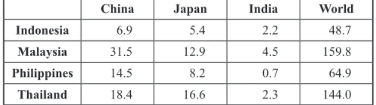
Table 1: Bilateral Trade as a Percentage of GDP for 2010-2014

　 China Japan India World

Indonesia 6.9 5.4 2.2 48.7

Malaysia 31.5 12.9 4.5 159.8

Philippines 14.5 8.2 0.7 64.9

Thailand 18.4 16.6 2.3 144.0

Source: Calculations are based on data from UN Commodity Trade Database and WB WDI.

Notes: The values are average of five years data as a percentage of GDP for each ASEAN country.

From 2010 to 2014, Indonesia’s average annual bilateral trade with major Asian economies was 14.5% of its GDP and 29.8% of its total foreign trade. The mentioned indicators were 48.9% and 30.6% for Malaysia, 23.4% and 36.1% for the Philippines, and 37.3% and 25.9% for Thailand (Table 1).

The flow of foreign direct investment (FDI) from the major Asian economies to ASEAN-4 was USD 28,738 million for 2010 to 2013, which included FDI of USD 4,608 million from China and USD 23,733 million from Japan. A significant volume of foreign trade and flow of FDI may cause a high correlation between the exchange rates of the major Asian economies and the ASEAN-4 economies (Table 2).

Table 2: FDI Flows from Major Economies to ASEAN-4 for 2010 ̶ 2013

　 China Japan India

Indonesia 2 155 7 879 168

Malaysia 458 3 790 229

Philippines 1 409 9 828 …

Thailand 586 2 236 …

Source: UNCTAD FDI/TNC database.

Notes: The values are in millions of U.S. dollars.

Changes and volatilities in the exchange rates of major Asian economies may significantly affect exchange rates of ASEAN-4 that do heavily depend on foreign trade with major Asian economies. Different issues related with exchange rates of various countries members of the ASEAN for the period of 2010 to 2015 were partially covered by some studies. In particular, Masujima (2015) estimated the quarterly equilibrium exchange rates of nine Asian currencies, including some ASEAN countries with the behavioral equilibrium exchange rates from 2006 to 2014. Kawai and Pontines (2014) examined the behavior of the Chinese RMB exchange rate and its impact on other currencies in emerging East Asia during the period 2000 to 2014. Soleymani and Chua (2014) investigated the impact of currency depreciation on bilateral trade between Malaysia and China over the period 1993 to 2012. Though, no previous empirical studies have exclusively analyzed dynamic interactions and causality relationship between exchange rates of ASEAN countries and three major Asian economies during the last five years.

The next two chapters present data and models used in estimations of dynamic conditional correlations, causality-in-mean and causality-in-variance between the logarithmic exchange rate return. Chapter four explains the findings from these estimations. The last chapter concludes the paper.

2. Data

Logarithmic return series of average weekly representative exchange rates are used for the estimations, based on the data reported by the IMF for the period from January 2, 2010, to July 25, 2015.

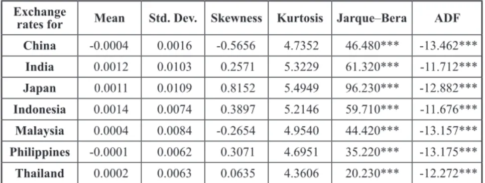
Descriptive statistics for the data are presented in Table 3. The mean and standard deviation of the variables are very close to zero. Skewness values for China and Malaysia show the distribution slightly skewed on the left, demonstrating longer tails on lower returns; for the other countries, the distribution is skewed on the right, demonstrating longer tails on higher returns. The kurtosis values are a little higher than the normal distribution. The Jarque–Bera test indicates that the null hypothesis of

‘normal distribution’ is rejected at the 1% significance level for all variables. The

standard Augmented Dickey–Fuller (ADF) test statistics (Dickey and Fuller 1979, 1981) reject the null hypothesis of a unit root at the 1% significance level. Data description justifies the use of Generalised Autoregressive Conditional Heteroscedasticity (GARCH) type models.

Table 3: Descriptive Statistics for Logarithmic Return Series Exchange

rates for Mean Std. Dev. Skewness Kurtosis Jarque–Bera ADF China -0.0004 0.0016 -0.5656 4.7352 46.480*** -13.462***

India 0.0012 0.0103 0.2571 5.3229 61.320*** -11.712***

Japan 0.0011 0.0109 0.8152 5.4949 96.230*** -12.882***

Indonesia 0.0014 0.0074 0.3897 5.2146 59.710*** -11.676***

Malaysia 0.0004 0.0084 -0.2654 4.9540 44.420*** -13.157***

Philippines -0.0001 0.0062 0.3071 4.6951 35.220*** -13.175***

Thailand 0.0002 0.0063 0.0635 4.3606 20.230*** -12.272***

Notes: *** in Jarque–Bera test indicate that the null hypothesis of “normal distribution”

is rejected at 1% significance level. *** in ADF mean smaller than the critical value at 1% significance level.

3. Methodology

First, we test structural changes for exchange rates returns series. Assuming the structural change points unknown, we make use of the test procedure proposed by Andrews (1993) and Andrews and Ploberger (1994). Based on Akaike’s information criterion (AIC), Bayesian information criterion (BIC) and log-likelihood ratio the dummy variables for structural breaks will be used in some equations of further estimations.

In the next step, we estimate the dynamic conditional correlation between exchange

rates returns of ASEAN-4 and major economies of Asia. We estimate the parameters of

dynamic conditional correlation (DCC) bivariate generalized autoregressive

conditionally heteroskedastic (GARCH) models (Bollerslev, 1986; Engle, 2002). The

mean equation of the model can be written as

t i t

t

Cx D

y = ω + + + ε ₍₁₎

The variance equation of the model can be written as

2

1 1 ,

2 , 2

, it j

p j

q

j j

j t i j i

t i

i

a

= − =

∑ ⁺ ∑

+

= ω ε β σ

σ . ₍₂₎

We model the conditional means of the returns as vector autoregressive (VAR) processes and the conditional co-variances as DCC-GARCH processes in which the variance of each disturbance term follows a GARCH(1,1) process. We use AIC, BIC, log-likelihood ratio and the Ljung–Box Q test to select the lag order for VAR and define the parameters of GARCH.

Variances and co-variance derived from the above equations are used in the estimation of the dynamic conditional correlation coefficients.

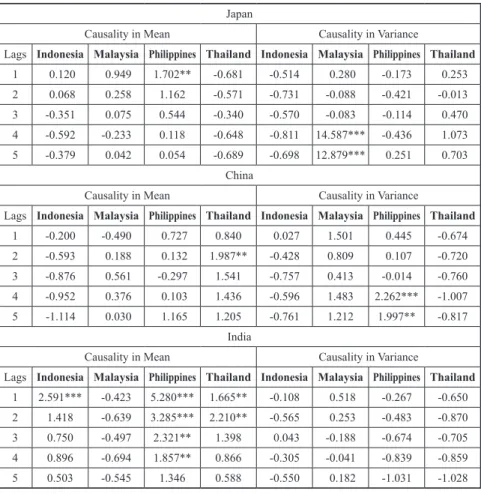
Finally, we use the cross-correlation function (CCF) approach developed by Cheung and Ng (1996) to examine the causal relationships in mean and variance between the logarithmic exchange rate returns. We use an autoregressive (AR) model and an exponential GARCH (EGARCH) model (Nelson, 1991) to calculate the conditional mean of

t i i t k

i i

t

a y D

y = ω + ∑

+ + ε ₍₃₎ and conditional variance

i i t p

i

q

i i

i t i i t i

t

⁾ = + ∑

⁽ z

+ ^(| z

^| − ^{2 / )} + ∑

^ln(

⁾ + D

ln( σ

ω

γ α π

β σ

, ₍₄₎

where z t = ε t ^/ σ t .

We use the standardized residuals from Equations 3 and 4 to test the causality in

mean and causality in variance applying CCF. A generalized version of Cheung and Ng

(1996) chi-square test statistic suggested by Hong (2001) with an asymptotic critical

value of 1.645 and 2.326 at the 5% and 1% levels are used to test the hypothesis of no

causality from lag 1 to a given lag of k in the cross-correlation coefficients.

4. Empirical Findings

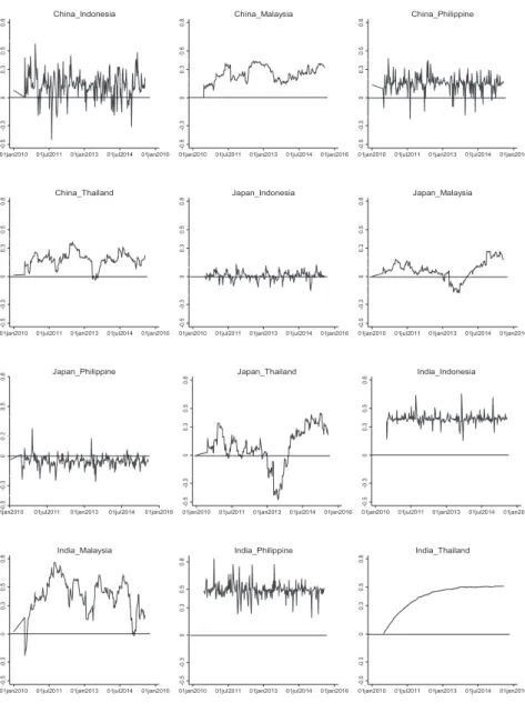
The dynamic conditional correlations between the exchange rate returns of China and ASEAN-4 are mostly positive and sufficiently high, ranging from the average minimum of -0.17 to the average maximum of 0.44, with an average mean of 0.18 and an average standard deviation of 0.09. In general, dynamic conditional correlation coefficients of China with Malaysia and Thailand are higher and less volatile, while those with Indonesia and Philippines are not as high but more volatile (Figure 1).

The dynamic conditional correlations between the exchange rate returns of Japan and ASEAN-4, in general, are not very high, ranging from an average minimum of -0.26 to an average maximum of 0.28, with an average mean of 0.03 and an average standard deviation of 0.10. The coefficients of dynamic conditional correlation with Indonesia are unstable and very close to zero, and those with the Philippines are also unstable and mostly negative. The coefficients of dynamic conditional correlation with Malaysia and Thailand are negative from April 6, 2013 to August 2, 2014, but high and positive thereafter.

The dynamic conditional correlations between the exchange rate returns of India

and ASEAN-4 are positive and high, ranging from the average minimum of 0.03 to the

average maximum of 0.67, with the average mean of 0.42 and average standard

deviation of 0.11. The conditional correlations coefficients with Malaysia and Thailand

have been increasing during the first two years. The coefficients with Thailand are the

most stable.

Figure 1: Dynamic Conditional Correlation between Exchange Rates Returns of Major Asian economies and ASEAN-4

A comparison of the coefficients of dynamic conditional correlations between the exchange rate returns of the major Asian economies and ASEAN-4 demonstrate a

00.60.80.50.3-0.3-0.5

01jan2010 01jul2011 01jan2013 01jul2014 01jan2016 China_Indonesia

00.40.30.20.10.30.80.5-0.5-0.3

01jan2010 01jul2011 01jan2013 01jul2014 01jan2016 China_Malaysia

00.40.2-0.20.30.50.8-0.5-0.3

01jan2010 01jul2011 01jan2013 01jul2014 01jan2016 China_Philippine

00.40.30.20.10.80.5-0.5-0.3

01jan2010 01jul2011 01jan2013 01jul2014 01jan2016 China_Thailand

00.1.1.1-.1.20.50.80.3-0.5-.2-0.3

01jan2010 01jul2011 01jan2013 01jul2014 01jan2016 Japan_Indonesia

00.30.8.20.5-0.3-.2-.1.1.2-0.5

01jan2010 01jul2011 01jan2013 01jul2014 01jan2016 Japan_Malaysia

0-0.40.20.5-0.3-0.5-.4.2-.2.40.8

01jan2010 01jul2011 01jan2013 01jul2014 01jan2016 Japan_Philippine

00.8-0.50.5-0.30.3

01jan2010 01jul2011 01jan2013 01jul2014 01jan2016 Japan_Thailand

0.50.30.8-0.5-0.30

01jan2010 01jul2011 01jan2013 01jul2014 01jan2016 India_Indonesia

00.80.50.3-0.3-0.5

01jan2010 01jul2011 01jan2013 01jul2014 01jan2016 India_Malaysia

0.80.30.5-0.5-0.30

01jan2010 01jul2011 01jan2013 01jul2014 01jan2016 India_Philippine

00.50.30.8-0.5-0.3

01jan2010 01jul2011 01jan2013 01jul2014 01jan2016 India_Thailand

higher interdependence for India and a lower interdependence for Japan as compared to China. The exchange rates of the Chinese RMB and the Indian rupee in comparison to the United States dollar are positively correlated with the exchange rates of the ASEAN-4’s national currencies. The exchange rate of the Japanese yen is not correlated with the Indonesian rupiah, negatively correlated with the Philippine peso, and positively correlated with the Malaysian ringgit and the Thai baht. The dynamic correlations between the exchange rates of China and ASEAN-4 seem consistent with the share of trade with, and the flow of FDI from, China. The same can be said about the correlation coefficients for Japan with ASEAN-4.

The empirical results for the AR-EGARCH models are presented in Table A1 (see Appendix). The number of lags for AR from one to three, and the dummy variables for structural change in the logarithmic return series, are included based on AIC and BIC.

The trends of the mean are significantly affected by the previous week’s returns, and the variation by the variations of returns in the previous week for all countries. The Ljung-Box Q statistics for the null hypothesis that there is no autocorrelation up to the order of 10 for standardised residuals and squared standardised residuals justify the empirical results of the AR-EGARCH models.

The standardised residuals and their squares derived from AR-EGARCH models are used for the estimation of causality-in-mean and causality-in-variance, based on the cross-correlation function (CCF). The test statistics indicate causality-in-mean from the Japanese yen to the Philippine peso, from the Chinese RMB to the Thai baht, and from the Indian rupee to the Indonesian rupiah, the Philippine peso and the Thai baht.

Causality-in-variance is indicated from the Japanese yen to the Malaysian ringgit, and from the Chinese RMB to the Philippine peso (Table 4).

The results of the causality test indicate that the exchange rate returns of the

Philippine peso are influenced by the exchange rate returns of the Japanese yen, those

of the Thai baht are influenced by the exchange rate returns of the Chinese RMB, and

those of the Indonesian rupiah, the Philippine peso and Thai baht are influenced by the

exchange rate returns of the Indian rupee. The volatilities in the exchange rate returns

of the Malaysian ringgit are influenced by changes in variances of the Japanese yen’s

exchange rate returns. On the other hand, the volatilities in the exchange rate returns of the Philippine peso are influenced by changes in variances of the Chinese RMB’s exchange rate returns.

Table 4: Test Statistics for Causality in Mean and Variance Based on CCF Japan

Causality in Mean Causality in Variance

Lags Indonesia　Malaysia Philippines Thailand Indonesia　Malaysia Philippines Thailand

1 0.120 0.949 1.702** -0.681 -0.514 0.280 -0.173 0.253

2 0.068 0.258 1.162 -0.571 -0.731 -0.088 -0.421 -0.013

3 -0.351 0.075 0.544 -0.340 -0.570 -0.083 -0.114 0.470

4 -0.592 -0.233 0.118 -0.648 -0.811 14.587*** -0.436 1.073

5 -0.379 0.042 0.054 -0.689 -0.698 12.879*** 0.251 0.703

China

Causality in Mean Causality in Variance

Lags Indonesia　Malaysia Philippines Thailand Indonesia　Malaysia Philippines Thailand

1 -0.200 -0.490 0.727 0.840 0.027 1.501 0.445 -0.674

2 -0.593 0.188 0.132 1.987** -0.428 0.809 0.107 -0.720

3 -0.876 0.561 -0.297 1.541 -0.757 0.413 -0.014 -0.760

4 -0.952 0.376 0.103 1.436 -0.596 1.483 2.262*** -1.007

5 -1.114 0.030 1.165 1.205 -0.761 1.212 1.997** -0.817

India

Causality in Mean Causality in Variance

Lags Indonesia　Malaysia Philippines Thailand Indonesia　Malaysia Philippines Thailand 1 2.591*** -0.423 5.280*** 1.665** -0.108 0.518 -0.267 -0.650

2 1.418 -0.639 3.285*** 2.210** -0.565 0.253 -0.483 -0.870

3 0.750 -0.497 2.321** 1.398 0.043 -0.188 -0.674 -0.705

4 0.896 -0.694 1.857** 0.866 -0.305 -0.041 -0.839 -0.859

5 0.503 -0.545 1.346 0.588 -0.550 0.182 -1.031 -1.028

Notes: ** and *** mean significance at the 5% and 1% levels.

5. Conclusion

In this paper, we estimated the dynamic conditional correlation, the causality-in-

mean and the causality-in-variance between the exchange rates of the three major Asian

economies and the four major economies of ASEAN (Indonesia, Malaysia, the Philippines and Thailand). The derived results from the estimations showed a sufficiently high dynamic correlation between the exchange rate returns of these countries, with the exception of Japan with Indonesia and Thailand. The causality-in- mean and causality-in-variance tests demonstrated that the exchange rates of the major economies of Asia exerted a significant influence on the Indonesian rupiah (affected by the Indian rupee), the Philippine peso (affected by the Japanese yen and the Indian rupee), and Thai baht (affected by the Chinese RMB and the Indian rupee). A significant influence of changes in variances of exchange rate returns was also demonstrated from the major Asian economies on the exchange rate return volatilities in Malaysia (affected by the Japanese yen) and the Philippines (affected by the Chinese RMB).

The derived results of the paper can be very much helpful for the investor’s decision and policy making in ASEAN-4. The findings can also be helpful for better understanding of the exchange rate behaviors and predicting the future movements of exchange rate markets of ASEAN-4.

Reference

Andrews, Donald W. K. 1993. “Tests for parameter instability and structural change with unknown change point.” Econometrica 61(4): 821–56.

http://dx.doi.org/10.2307/2951764

Andrews, Donald W. K. and Werner Ploberger. 1994. “Optimal tests when a nuisance parameter is present only under the alternative.” Econometrica 62(6): 1383–14.

http://dx.doi.org/10.2307/2951753

Bollerslev, Tim. 1986. “Generalised autoregressive conditional hetroscedasticity.”

Journal of Econometrics 31: 307–27.

http://dx.doi.org/10.1016/0304-4076(86)90063-1

Cheung, Yin-Wong and Lilian K. Ng. 1996. “A causality-in-variance test and its application to financial markets prices.” Journal of Econometrics 72(1): 33–48.

http://dx.doi.org/10.1016/0304-4076(94)01714-X

Dickey A. David and Fuller A. Wayne. 1979. “Distribution of the estimators for autoregressive time series with a unit root.” Journal of the American Statistical Association 74(366): 427–31.

http://dx.doi.org/10.2307/2286348

Dickey A. David and Fuller A. Wayne. 1981. “Likelihood ration statistics for autoregressive time series with a unit root.” Econometrica 49(4): 1057–72.

http://dx.doi.org/10.2307/1912517

DNA. 2015. “India clocks 7.5% growth in January-March quarter, becomes world’s fastest growing economy.” 29 May 2015. New Delhi, PTI.

Engle F. Robert. 2002. “Dynamic conditional correlation: A simple class of multivariate generalized autoregressive conditional hetroscedasticity models.” Journal of Business and Economic Statistics 20(3): 339–50.

http://dx.doi.org/10.1198/073500102288618487

Henning, R. 2012. “Choice and coercion in East Asian exchange rate regimes.”

Working Paper 12–15. Washington: Peterson Institute for International Economics.

Hong, Y. 2001. “A test for volatility spillover with application to exchange rates.”

Journal of Econometrics 103(1-2): 183–24.

http://dx.doi.org/10.1016/S0304-4076(01)00043-4

International Monetary Fund. 2014. “Annual report on exchange arrangements and exchange restrictions.” Washington, October.

https://www.imf.org/external/pubs/nft/2014/areaers/ar2014.pdf

Kawai, Masahiro and Victor Pontines. 2014. “The Renminbi and exchange rate regimes in East Asia.” ADBI Working Paper 484. Tokyo: Asian Development Bank Institute. http://www.adbi.org/working-paper/2014/05/30/6303.renminbi.

exchange.rate/

Nelson, Daniel B. 1991. “The conditional heteroskedasticity in asset returns: A new approach.” Econometrica 59(2): 347–70.

http://dx.doi.org/10.2307/2938260

Ohno, Kenichi. 2006. “The economic development of Japan: The path traveled by

Japan as a developing country.” GRIPS Development Forum, National Graduate Institute for Policy Studies.

http://www.grips.ac.jp/vietnam/KOarchives/download_E.htm

Soleymani, Abdorreza and Soo Y. Chua. 2014. “How responsive are trade flows between Malaysia and China to the exchange rate? Evidence from industry data.” International Review of Applied Economics 28: 191–09.

http://dx.doi.org/10.1080/02692171.2013.858666

The Guardian. (2011). “China overtakes Japan as world’s second-largest economy.”

Justin McCurry and Julia Kollewe. 14 Feb. 2011.

http://www.theguardian.com/business/2011/feb/14/china-second-largest- economy

World Bank. 2015. World Development Indicators: GDP growth, annual percentage.

Retrieved November 1, 2015. http://data.worldbank.org/indicator/NY.GDP.

MKTP.KD.ZG

World Bank. 2015. World Development Indicators: GDP, current U.S. dollars.

Retrieved November 1, 2015.

http://data.worldbank.org/indicator/NY.GDP.MKTP.CD

Masujima, Yuki. 2015. “Assessing Asian Equilibrium Exchange Rates as Policy

Instruments.” Discussion papers 15038, Research Institute of Economy, Trade

and Industry (RIETI).

Appendix

Table A1: Results of the AR-EGARCH Models

Japan China India Indonesia Malaysia Philippines Thailand Mean

a ₁ ^0.1773*** _{(0.0653) (0.0652)} ^{0.0596 0.2550***} _(0.0551) ^0.2523*** _(0.0488) ^0.1405*** _(0.0541) ^0.1602** _(0.0662) ^0.2468*** _(0.0536)

a _{2 (0.0605)} ^-0.0382

a _{3 (0.0613)} ^0.0174

D 0.004***

(0.021) 0.0008***

(00002) Constant -0.0021** (0.0009) -0.0009***

(0.0002) 0.0009*

(0.0005) 0.0006***

(0.0002) 0.0003

(0.0005) 0.0001

(0.0003) 0.0001 (0.0003) Variance

α 1 0.0358

(0.0678) 0.2655**

(0.1081) 0.0413

(0.0702) 0.2901***

(0.1090) 0.0831

(0.0889) 0.2086

(0.1414) 0.1532 (0.1803)

γ 1 0.1845***

(0.0585) 0.0576

(0.0700) 0.1387***

(0.0388) 0.1258*

(0.0662) 0.1090*

(0.0613) -0.0294

(0.0779) 0.1320 (0.1072)

β 1 0.9298***

(0.0276) 0.9321***

(0.0575) 0.9735***

(0.0164) 0.9414***

(0.0347) 0.9168***

(0.0572) 0.8679***

(0.1414) 0.6655**

(0.2649)

ω ^-0.6556*** _{(0.2548) (0.7497)} ^{-0.8818 -0.2542*} _{(0.1535) (0.3554)} ^-0.5779 _(0.5573) ^-0.8093 _(1.4554) ^-1.3489 _(2.7042) ^-3.4152

parameter GED 0.4542***

(0.1009) 0.3484**

(0.1362) 0.3581***

(0.1375) -0.0005

(0.1201) 0.4151***

(0.1258) 0.3483***

(0.1252) 0.1191 (0.1407) Diagnostic

Q ⁽¹⁰⁾ _(0.8593) ^5.4480 _(0.0712) ^17.1436 _(0.8719) ^5.2772 _(0.5127) ^9.2054 _(0.5678) ^8.6278 _(0.1709) ^14.0459 _(0.4655) ^9.7186 Q ^{2 (10)} _(0.9813) ^3.0032 _(0.7583) ^6.6470 _(0.9981) ^1.7161 _(0.9284) ^4.3842 _(0.6418) ^7.8673 _(0.4418) ^9.9846 _(0.8758) ^5.2235 Notes: The numbers in parentheses are standard errors. Q (10) and squared Q (10) are

the Ljung–Box Q statistics for the null hypothesis that there is no autocorrelation up to orders 10 for standardized residuals and squared standardized residuals. *, ** and *** mean significance at the 10%, 5% and 1%

levels.