Theoretical studies of the formation mechanism of protein complex by using coarse-grained models

Theoretical studies of the formation mechanism of protein complex by using coarse‑grained

models

著者 ミケ ルスメリヤニ

著者別表示 Miche Rusmerryani journal or

publication title

博士論文本文Full 学位授与番号 13301甲第4142号

学位名 博士（理学）

学位授与年月日 2014‑09‑26

URL http://hdl.handle.net/2297/40539

Theoretical Studies of the Formation Mechanism of Protein Complex by

Using Coarse-grained Models

Micke Rusmerryani

Division of Mathematical and Physical Science, Graduate School of Natural Science and Technology,

Kanazawa University

2014

博士論文

粗視化 モデルを 用 いたタンパク 質複合体形 成機構 に 関 する 理論的研究

金沢大学大学院自然科学研究科 数物科学専攻

計算バイオ研究室

学籍番号

1123102010

氏名

Micke Rusmerryani

主任指導教員氏名 長尾秀実

Acknowledgement

First of all, I would like to express my deepest gratitude to the one above all of us, the omnipresent Allah SWT, for answering my prayers and for giving me the strength to accomplish this doctoral thesis.

In this occasion, I would like to offer my sincerest gratitude to my super- visor, Prof. Hidemi Nagao, who not only served as my supervisor but also encouraged and challenged me throughout my academic program. The good advice, support and valuable discussions on both an academic and a personal level from Prof. Masako Takasu, for which I am extremely grate- ful. I also would like to gratitude Assistant Professor Hiroaki Saito, Assistant Professor Kazutomo Kawaguchi, and Dr. Acep Purqon for the kindness, supports, and helps me a lot not only in academic but also in my life. Also to Prof. Mineo Saito, Prof. Tatsuki Oda, and Prof. Shinichi Miura, for the valuable advices and supports.

Many thanks are given to all my members of the Computational Bio- physics Laboratory for kindly supports and encouragements to make this work possible. To Seiji Matsui and Hikmah Balbeid who always support me through good time and bad time. To all members of PPI Ishikawa and Berang for many helps and enjoyable moments. It is a pleasure to thank those who made this thesis possible, hence I apologize I can not write all the names but I will always remember all your kindness.

Last but not the least, I dedicate this thesis to my parents who have given

me the opportunity of an education from the best institutions and support

throughout my life and to my family and Dendi who gave me their unequivo-

cal support.

Contents

Acknowledgement i

Contents ii

List of Figures v

List of Tables vii

1 Introduction 1

1.1 Motivation . . . . 1

1.2 Overview of the thesis . . . . 2

2 Research Objectives 4 2.1 Azurin . . . . 4

2.2 Coarse-grained models . . . . 8

3 Implementation of Coarse-Grained Model to Probe Unfolding Pro- cess of Azurin 11 3.1 Introduction . . . . 11

3.2 Material and methods . . . . 13

3.2.1 Protein . . . . 13

3.2.2 Coarse-grained model of protein . . . . 14

3.2.3 Unit of coarse-grained model . . . . 14

3.2.4 Potential model . . . . 14

3.2.5 Equation of motion . . . . 17

3.3 Analysis methods . . . . 17

3.3.1 Measure of nativeness . . . . 18

3.3.2

18

3.4 Results . . . . 19

3.5 Conclusion . . . . 24

4 Implementation of G ¯ o Model on Azurin Complex System 25 4.1 Introduction . . . . 25

4.2 Material and simulation methods . . . . 26

4.2.1 Model system . . . . 26

4.2.2 Potential model . . . . 28

4.2.3 Simulation condition . . . . 28

4.3 Analysis methods . . . . 29

4.4 Results . . . . 29

4.5 Conclusions . . . . 33

5 The Effects of Intermolecular Interactions to The Conformational Changes of Azurin Complex 34 5.1 Introduction . . . . 34

5.2 Material and simulation methods . . . . 35

5.2.1 Model systems . . . . 35

5.2.2 Potential model . . . . 37

5.2.3 Simulation condition . . . . 37

5.3 Analysis methods . . . . 39

5.4 Results . . . . 39

5.5 Conclusion . . . . 46

6 General Conclusion 47 Appendix A Extended research: An improved coarse-grained model of azurin complex via bottom-up approach 49 A.1 Introduction . . . . 49

A.2 Material and simulation methods . . . . 50

A.2.1 Model systems . . . . 50

A.2.2 Potential model . . . . 50

A.3 Analysis methods . . . . 54

A.4 Results . . . . 55

A.5 Conclusion . . . . 60

Appendix B Force field 61 B.1 G ¯o potential . . . . 61

B.2 6-12 Lennard-Jones potential . . . . 68

B.3 Modified Lennard-Jones potential . . . . 68

List of publications 69 Papers as first author . . . . 69

Other papers . . . . 69

References 70

List of Figures

2.1 Three dimensional structure of azurin complex obtained from X-ray crystal structure (PDB entry : 4AZU) . . . . 6 2.2 Topology of the Greek key motif. . . . 6 2.3 Structure of Pseudomonas aeruginosa azurin containing Greek

key motif . . . . 7 3.1 Comparison of free energy as a function of reaction coordi-

nate Q between mutated azurin and wild-type . . . . 21 3.2 Comparison of

azurin and wild-type azurin at T

T

. . . . 23 4.1 Initial configurations. . . . 27 4.2 Time series of the interchain distances. . . . 30 4.3 Autocorrelation of the interchain distance as a function of time

lag (τ ). . . . 31 4.4 Free energy profile as a function of reaction coordinate Q

which is the measurement of the nativeness. . . . 32 5.1 Various initial conformations. System I, II, and III are dimer

systems with different contact orientation. . . . 36 5.2 The root mean square displacement shows the conforma-

tional changes compared to the given initial configuration . . 40 5.3 The total surface area is calculated at the residue level and is

normalized by the total surface area of independent chains . 40

5.4 The root mean square displacement of the simulations with

ε

kcal/mol. . . . . 41

5.5 The normalized total surface area of the simulations with ε

kcal/mol. . . . 43

5.6 The regression of normalized surface to the ratio of number of pair contacts . . . . 44

5.7 Number of contacts in the binding area . . . . 45

A.1 Snapshots of the tetramer azurin from our simulation. . . . . 55

A.2 RMSD profile for whole system. . . . 56

A.3 RMSD profile for each chain. . . . 56

A.4 RMSF profile for each chain. . . . 58

A.5 RMSF profile for each chain from all atom simulation. . . . . 58

A.6 Number of intermolecular contact. . . . 59

A.7 Total surface area . . . . 59

List of Tables

3.1 Units of coarse-grained model . . . . 14

3.2 Potential model . . . . 16

3.3 Potential parameter . . . . 16

4.1 Standard deviation of the interchain distances . . . . 31

5.1 New units of coarse-grained model . . . . 37

5.2 Potential parameter and simulation condition . . . . 38

5.3 Comparison of two non-bonded potential . . . . 38

5.4 Quantitative comparison of the RMSD of each system is rep- resented by the calculation of average (Å) and standard devi- ation (Å) of RMSD. . . . 42

5.5 Comparison of the initial and average surface area (Å

), initial

number of pair contacts, and average total energy (kcal/mol). 42

A.1 Van der Waals radii (in Å) for 20 amino acids . . . . 53

Chapter 1 Introduction

1.1 Motivation

My current research is inspired by the rapid developments of nanoscience in the last decade. The concept of nanoscience was first addressed by physicist Richard Feynman in his lecture "There’s Plenty of Room at the Bottom" [1]. In his talk, he considered a feasibility to manipulate matter on an atomic scale and offered some challenges which are known later as nanotechnology.

In this universe, all matter is built up of extremelly small particles called atoms. Since nanoscience deals with the nanomaterials, it requires the abi- lity to imagine, observe, and work on the nanoscale, where the prefix "nano"

refers to

.

Nevertheless, both experimental and theoretical studies on behavior of nanomaterials are still limited. For instance, to see such an extremely small matter like atom, we need the most advanced microscope, the scanning tunneling microscope (STM). Recently, computer simulation has emerged as the midway between the theoretical and experimental approaches to ob- tain better understanding of matter on the atomic scale.

In particular, my research interest lies in the field of biomolecular mode-

ling and more specifically in the study of the formation of protein complex.

organism is made up of cells. To understand the properties of the cell, it is important to understand how the atoms or molecules attract and bind to another to form a cell.

One of the most common computational methods for studying the dyna- mics of protein in atomic scale is molecular dynamics simulation. Although molecular dynamics simulation allow us to observe the protein dynamics in atomic details, it is limited to the size and time scales. In order to surpass these limitations, in this thesis I try to extend the biomolecular modeling to study the protein complex dynamics.

1.2 Overview of the thesis

This thesis is organized as follows:

Chapter 1 gives general introduction consisting of motivation of my research and overview of this thesis.

In chapter 2, we introduce the basic information of azurin including the struc- ture and the biological functions. We also introduce the basic concept of coarse-graining in biomolecular modeling.

The next three chapters are presented based on my published papers as first author. In chapter 3, we present our study on unfolding process of azurin using native-center structure based model. The paper is:

M. Rusmerryani, M. T. Pakpahan, M. Nishimura, M . Takasu, K.

Kawaguchi, H. Saito, and H. Nagao. Transition state analysis of azurin via G ¯o-like model, AIP Conf. Proc., 1518, 641 (2013).

In chapter 4, we expand this model to simulate several chains of azurin. The

paper is:

M. Rusmerryani, M . Takasu, K. Kawaguchi, H. Saito, and H. Nagao.

Coarse-grained simulation of azurin crystal complex system: Protein–

protein interactions, ISCS 2013 Selected Papers, 4 (2013).

In chapter 5, we improve our model by using Lennard-Jones potential as the intermolecular interaction in order to find more transferable coarse-grained model. The paper is:

M. Rusmerryani, M . Takasu, K. Kawaguchi, H. Saito, and H. Nagao.

Protein–protein interactions of azurin complex by coarse-grained simu- lations with a G ¯o-like model, JPS Conf. Proc., 1, 012054 (2014).

Chapter 6 is conclusion of this thesis and future work.

Moreover, in Appendix B we present our extended work which will be

submitted. In this work, we employ knowledge-based approach by empir-

ically evaluate the intermolecular contacts from known crystal structure of

azurin. This work will offer a new insight to approach the intermolecular

potential model for unknown complex structure. Last, in Appendix A we

provide brief derivation of our force field.

Chapter 2

Research Objectives

In the following sections we will briefly introduce the main objectives for our research: protein azurin and coarse-grained models in the field of bio- molecular modeling.

2.1 Azurin

Azurin is one of cupredoxin or blue copper protein that contains a single Type I copper center. Azurin molecule has low molecular weight around 14 kDa and consists of 128 amino acids [2]. Azurin is found mainly in Pseu- domonas aeruginosa bacteria [3] which usually grows in the soil but also often found in the lungs. Azurin from Pseudomonas aeruginosa is known to exhibit a large stability [4].

As other cupredoxins, azurin functions in the electron transfer. Particu- larly, the electron transfers occur between azurin and cytochrome c-551 [5]

and between azurin and cytochrome c oxidase [6]. Advanced studies have been conducted both experimentally and theoretically for further investiga- tion of the kinetics of electron transfer.

Recently, many researches put their attention to investigate azurin since

azurin may be considered as a proper candidate for treatment of cancer

through nanotechnology [7]. Azurin was found to form a complex with the

tumor-suppressor protein p53 [8] and to induce apoptosis in macrophage

cells [9]. Several studies on cancer treatment by azurin are performed, in- cluding melanoma [9], breast cancer [10, 11], bone cancer [12], prostate cancer [13], brain tumor [13], and leukemia cells treatment [14].

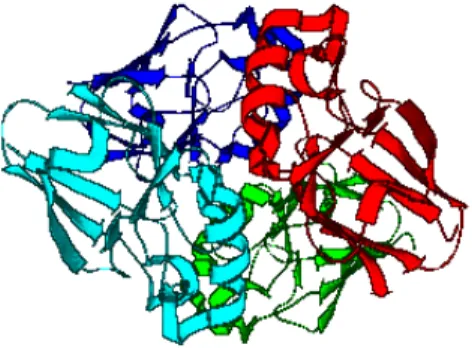
In this thesis, we use the native structure of azurin complex system obtained from X-ray crystal structure of Pseudomonas Aeruginosa azurin (PDB entry : 4AZU) [15]. In this azurin complex, the unit cell

consists of one asymmetric unit

where its asymmetric unit is composed of a tetramer of azurin molecules (Figure 2.1).

Each azurin is composed of eight β-strands and one helix arranged in a double wound Greek key topology [16]. A Greek key is a series of four se- quential β-strands arranged in the order three up-and-down β-strands con- nected by hairpins are followed by a longer connection to the fourth strand which lies adjacent to the first (Figure 2.2). The structure of azurin contain- ing Greek key motif can be seen in Figure 2.3. The copper is coordinated by three strong ligands arranged in a trigonal-planar configuration (the side chains of Cys112, His117, and His46) and a weak ligand Met121. However, in this thesis the interaction made by copper will be neglected.

1Unit cellis the smallest building block of a crystal structure

2Asymmetric unit is the smallest part of the crystal that is duplicated and moved by

Figure 2.1: Three dimensional structure of azurin complex obtained from X-ray crystal structure of Pseudomonas Aeruginosa azurin (PDB entry : 4AZU)

Figure 2.2: Topology of the Greek key motif.

(a) Topology diagram

(b) Three dimensional structure

Figure 2.3: Structure of Pseudomonas aeruginosa azurin containing Greek

key motif showing in simplified topology diagram (a) and in real three dimen-

sional structure generated by VMD (b).

2.2 Coarse-grained models

Coarse-grained model is a lower resolution model where some of fine details are eliminated. In molecular dynamics, this model is obtained by replacing the "unnecessary" atomistic details of a biological molecule. In the past decade, coarse-grained models have gained much attention since they could overcome the spatial and temporal problems of all-atom model. All- atom simulations are limited to small systems and nanosecond time scales.

Meanwhile, coarse-grained models allow us to simulate larger systems and slow processes which require micro- to millisecond time scales.

Several coarse-grained models have been developed for many classes of biomolecules: water, lipids [17–20], proteins [21–26], nucleic acids, and carbohydrates. These models are constructed with different levels of reso- lution and approaches. As the current work deals with protein, now we only discuss coarse-grained protein models and introduce several models that have been quite successful to characterize protein folding and dynamics.

To construct a coarse-grained model, first we have to determine the re- solution of the representation for our system. In coarse-grained protein mo- dels, each amino acid can be represented by one site, usually associated with the position of α-carbon, or a few sites, usually three or more back- bone sites. After that, we have to determine the appropriate interactions between coarse-grained particles. This part has become a great challenge in biomolecular modeling.

There are several approaches to develop the coarse-grained potentials.

The most common way is to classify these approaches into top-down and

bottom-up approaches. In bottom-up approaches, the interaction between

coarse-grained particles is determined based upon the given fundamental

description from a higher resolution model or classical atomistic model for

the same system. Conversely, top-down models is constructed on the basis

of the real experimental observation that provides the phenomena of physi-

cal principles, especially the thermodynamics properties.

These approaches have their own advantages and disadvantages. Bottom- up models can be used to predict the particular system when no such ob- servation exist. On the other hand, while their models are restricted to their dependence on the more detailed model, the top-down models are typi- cally under-constrained, which means that the restrictions are very small.

Nevertheless, as the advancement of coarse-grained models may integrate both principles, the distinction becomes quite intuitive and blurred. For in- stance, the popular Martini model has retained a great success in providing transferable potential for modeling liquid and membrane by incorporating the top-down and bottom-up approach [27, 28].

Another common way is to distinguish them into physics-based and knowledge-based approaches. While the physics-based approaches em- ploy physical theories to determine the interaction, the knowledge-based approaches employ the empirical informations provided from the experi- mentally determined three-dimensional structure. This distinction is also becoming blurred with the same reason. Most coarse-grained models for protein usually combine these two approaches with bottom-up approach.

Several models have been successfully applied to study the dynamics of protein. The simplest coarse-grained protein model is network model, such as Elastic Network Model (ENM) [29] or Gaussian Network Model (GNM) [30]. These models determine their coefficients based on the na- tive contact map and employ a spring potential for modeling all interactions.

Nevertheless, these models do not provide the directions of particle motions.

Native-centric models also have been greatly used to study the protein folding. Similar to the network models, native-centric model also determine the parameters on the basis of the native contacts. This model, usually referred as G ¯o model, represents the interaction as bonded and non-bonded interactions [21]. At this time, this model may be the most realistic coarse- grained model for protein. However, these models can not be applied to the unknown structure.

Other promising knowledge-based models have been developed to pro-

vide more transferable coarse-grained model. The best known model is Miyazawa and Jernigan model with the statistical contact potentials. This model has widely been used as a first estimate of the interaction between particles in coarse-grained model [23,31,32]. On the implementation, people usually combine those models with bottom-up approach to construct the po- tential strength. The commonly used strategies are Iterative Boltzmann In- version (IBI) [33], Inverse Monte Carlo (IMC) [34], and the Force-Matching [35, 36].

After all, that is why the coarse-grained is favored for solving many bio-

molecular problems. The flexibility to improve their models by integrating

several approaches based on their research purposes has become a great

advantage of coarse-grained. This way researchers can optimize the effec-

tiveness of their models.

Chapter 3

Implementation of

Coarse-Grained Model to Probe Unfolding Process of Azurin

In this chapter, we employ our structure-based coarse-grained simulation by adopting G ¯o potential model to examine the effects of mutated azurin to the unfolding process.

3.1 Introduction

Protein assembles to the unique three-dimensional structure called the native state to perform its biological function. The understanding of con- formational transition from denatured to native state, or usually known as folding process, is very important. While the native state is unique, the tran- sition state is not just a single conformation. Multiple folding pathways can lead the protein sequences toward the native state or in contrast the path- ways may be trapped in the non-native conformation.

The study of protein folding was pioneered by Anfinsen [37] on his obser-

vation on the refolding of ribonuclease molecule. His famous “Thermody-

namic Hypothesis” has become a fundamental keystone to the develop-

ment on the study of protein folding. Its statement that the native structure

of an amino acid sequence in its normal surrounding is the one which has the lowest free energy, also has been supported by the funneled energy landscape theory [38].

In recent times, major developments on the study of protein folding dyna- mics has been greatly advanced into the fast and time-resolved techniques.

Along with the prior advances in the experimental and theoretical studies, those studies can be combined to develop the computational studies of fold- ing mechanism at the residue or atomic level. For instance, structure-based simulation, pioneered by G ¯o [21], has successfully employed underlying two essential theories of folding mechanism: the principle of minimal frustra- tion [39] and the funneled energy landscape [38, 40]. In addition, transition state theory also has been widely used to probe the folding/unfolding mech- anism with the computational studies [41,42]. Together, the structure-based simulation and transition state theory have become powerful tools to exam- ine the folding/unfolding process in the multiscale level.

In the last decade, understanding the effects of mutation on protein is one of great issues both in experimental and computational studies. It will provide many valuable insights to understand stability and kinetics of protein such as azurin. In this chapter, we will discuss our coarse-grained simulation on azurin. Azurin is known as an extremely stable protein as (see Section 2.1 for further explanation). However, experimental study of mutated azurin was found that the mutation of His117 to Gly on the apo-form affects the sta- bility of azurin whereas the unfolding proceeds much faster [43]. Currently, we implement the off-lattice G ¯o-like potential [21, 22] to probe the unfolding dynamics of a mutated azurin and a wild-type azurin.

Experimentally, azurin is known to exhibit two-state folding/unfolding pro-

cess: native and denatured states [44]. Here, we observed the change in ac-

tivation free energy relative to the change in stability of the transition state to

locate three state ensemble and compared with the wild-type azurin. More-

over, we also considered how the temperature affects the unfolding process

of this mutated azurin. For structural description, we probed the unfolding

pathways of azurin using protein engineering technique,

sult has found to be in agreement with both experimental and theoretical data. Present study also shows that the helix region, known as p28 peptide fragment of azurin, remains stable in both mutated and wild-type azurin.

3.2 Material and methods

Protein folding/unfolding is a process of unstructured (unfolded) amino acid sequences transforming into structured state or usually called native state, and vice versa. To understand the folding mechanism, sometimes we need to observe the unfolding mechanism beforehand. In this study, we probe the unfolding mechanism of a mutated azurin and compare it to the wild-type azurin via coarse-grained simulation. More detailed explanation of our model system and simulation method is given below.

3.2.1 Protein

As described in Chapter I, we limit our objective by observing dynamics of azurin. In this chapter, we choose the mutated azurin obtained by chang- ing His117 for a glycine. His117 is one of the three main ligands on the cop- per binding site. This mutation increases the flexibility on the loop containing those ligands and is less rigid compared to the wild-type azurin. Regarding to the folding process, the folding speed of the mutated azurin is known to be quite similar to the wild-type azurin. In contrast, the unfolding speed is found to be faster than the wild-type [43].

Currently, we simulate single apo-azurin for both mutated and wild-type azurin. The initial structures are taken from protein data bank

with PDB ID:

3N2J for H117G azurin [45] and 4AZU for wild-type azurin [15]. The crystal structures of both azurins are almost the same since the position of residue 117 is on the loop which is out of the main β-strand of the azurin.

1http://www.rscb.org/

3.2.2 Coarse-grained model of protein

The basic concept of coarse-graining is to simplify high-resolution details that are not necessary to understand the particular process. Coarse-grained models of biomolecules usually represent groupings of two or more atoms into a single bead. In our study, we develop coarse-grained model of protein at the residue level in which each residue is represented only with C

atoms.

We set each particle with the same mass.

3.2.3 Unit of coarse-grained model

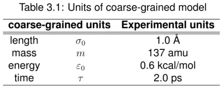
We determine the units for our coarse-grained model using basic quanti- ties, which are length (σ

), mass (m), time (τ ), and derived quantity, energy (ε

). The values of our coarse-grained units are listed in Table 3.1. The val- ues of σ

, m, and ε

are determined from the radius of protein, the average mass of amino acids, and the temperature of system, respectively. Mean- while, the time unit (τ ) is calculated by σ

p

m/ε

.

3.2.4 Potential model

We applied the off-lattice model founded by G ¯o [21] to mimic the perfect funnel aspect of folding energy landscape for our coarse-grained model.

We adapt G ¯o model interaction energy which is developed by Clementi et

Table 3.1: Units of coarse-grained model coarse-grained units Experimental units

length σ

1.0 Å

mass m 137 amu

energy ε

0.6 kcal/mol

time τ 2.0 ps

al. [22]. This model explicitly maintains the stability of native contacts by eliminating the energetic frustration from the non-native interactions. Until now, this model has retained great success on the folding studies.

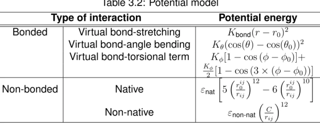
The potential energy between particles involves bonded and nonbonded interaction energy as shown in detail in Table 3.2. Bonded potential energy between particles describes spring potential for two successive particles, angle potential energy describes bending motion between two successive virtual-bonds, and dihedral potential describes the rotation of the four sub- sequent residues. Meanwhile, nonbonded interaction is distinguished into two categories, native interaction and non-native interaction.

In Table 3.2, r, θ, and φ represent the distance between two successive residues, the angles formed by three successive particles, and the dihe- dral angle defined by four subsequent residues along the chain at the given configuration, respectively. The non-bonded interaction implement 10-12 Lennard-Jones potential for native interactions and a short-range repulsive between non-native pairs, where r

represents the distance between i-th and j -th unsubsequent residues. We define a pair to be in native contact if r

is less than

Å. Otherwise, it will be categorized as non-native pairs.

All variables with subscript "0" mean the values of the corresponding vari-

ables at the native conformation. Detailed potential parameters are shown

in Table 3.3.

Table 3.2: Potential model

Type of interaction Potential energy Bonded Virtual bond-stretching K

r

Virtual bond-angle bending K

Virtual bond-torsional term K

φ

Kφ

2 [1−cos (3×(φ−

φ

Non-bonded Native ε

5_rij

0

rij

12

−6_rij 0

rij

10

Non-native ε

C rij

12

Table 3.3: Potential parameter

Parameter Value in kcal/mol Virtual bond-stretching K

Å

Virtual bond-angle bending K

Virtual bond-torsional term K

Native ε

Non-native ε

3.2.5 Equation of motion

The main idea of our simulation is to predict the dynamics of the protein.

For every time step, the position and velocity of each residue are calculated using Newton’s second law:

m d

~ r

dt

F , ~ (3.1)

where ~ r is the vector of Cartesian coordinate of the particle, and F ~ is the gradient of the potential energy at the given particle. In our coarse-grained simulation, we implement the Langevin equation of motion to mimic the non- conservative forces from the solvent which is describe in the following equa- tion:

m d

~ r

dt

F ~

ζ d~ r

dt

ξ(t), (3.2)

where ζ, the damping friction coeffient, is set to be

ξ(t) represents the random force which satisfy:

hξ(t)i= 0;

(3.3)

hξ(t)ξ(t⁰)i= 2mζk_B

T δ(t

t

(3.4) where k

is the Boltzmann constant.

We use the simple and widely used numerical integration algorithm, leap- frog algorithm, to solve the equation 3.2. Then the position and velocity of each particle can be obtained. This algorithm is computationally less expen- sive and less "storage consuming" than the predictor-corrector algorithm, yet is still accurate.

3.3 Analysis methods

The kinetic free energy relation can be used to obtain the position of

the funnel transition state [38, 41, 42]. While the native state is unique, the

transition state is not just a single conformation which can be defined as an ensemble. The transition state ensemble (TSE) consists of relatively large number of configurations described by specific order parameter that measures its nativeness. Most of small proteins have a two-state fold- ing/unfolding process. In such a case, three states appear and are defined as: native, transition, and denatured states.

3.3.1 Measure of nativeness

One way to measure the nativeness of the given configuration is by the fraction of the native contacts [38]. A pair residue is counted to be in native contact if the distance is less than 6.5 Å in the native state. Related to the kinetic free energy, this order parameter also can be defined as the reaction coordinate. For our convenience, we define it as Q, which mathematically can be written as

Q

number of native contacts in a given configuration

number of native contacts in native state . (3.5) This value of Q ranges from 0 to 1, in which Q close to unity represents the similarity to the native structure. In reverse, Q close to zero shows the dissimilarity to the native structure.

By the histogram method, the free energy profile (F

tained [46]. The relation between free energy and the position of the funnel transition state allows us to locate the three states ensemble, which are denatured, transition, and native state.

3.3.2 Φ-analysis

The free energy profile is a good tool to provide us the general descrip-

tion of the funnel of transition state. Nevertheless, it does not provide us

structural description. Therefore, further analysis is needed to characterize

the TSE. In experimental studies, currently the only way to probe the transi-

tion state of the folding process in depth is the protein engineering method,

Φ-analysis. It is defined as the ratio of change of the folding barrier energy

to stability upon the mutations, which is represented by following equation

Φ = ∆∆G^‡

∆∆G⁰

, (3.6)

where

is the difference in the total free energy between mutant and wild-type proteins, and

is the free energy changes of the folding bar- rier.

In the same objective, the theoretical

by Fersht and colleagues [47, 48] to characterize the TSE. This technique has been successfully applied to analyze folding TSE [22,49]. The change in free energy barrier can be interpreted by a single simple reaction coordinate.

Then, the

Φ_i = hE_ii_{T S}− hE_ii_D hEiiN − hEiiD

, (3.7)

where E

is the sum of interaction energies of i-th residue with any other re- sidues and the bracket

means average of the quantity over an ensemble.

The subscripts represent its states: TS, D, and N, for transition, denatured, and native state, respectively.

This statistical mechanical description of

has been widely used for comparison with the experimental

file allows us to locate the TSE,

residue at the transition state. Besides, it also can be used to measure the changes in TSE upon single or multiple mutations on the folding rate and stability.

3.4 Results

Several short simulations are performed under various temperatures,

chosen by bisection method over range of temperatures, to estimate the

folding transition temperature (T ). We start with the low temperature which

gives us high population of native state (high Q) and also the high tempera- ture which gives the opposite condition. Then we select the subinterval to narrow the range of temperature. Repeatedly we apply the bisection method over the new subinterval until the criteria for folding transition temperature is satisfied. The folding transition temperature itself is determined when the native state and denatured state are equipopulated. The folding tempera- ture of wild type azurin is considered to be referenced to a set of states.

Then several simulations of mutated azurin are performed under constant temperatures: T

T

, T < T

, and T > T

, for longer simulation time.

In order to obtain the free energy profile, we observed the thermody- namic configurations as a function of the reaction coordinate along simula- tion time which is represented by the fraction of native contacts formed in a given conformation as we mentioned in the previous section. At the T

, the Q-score fluctuates along simulation and almost equipopulated between native and denatured states. In the native structure, 186 contacts exist.

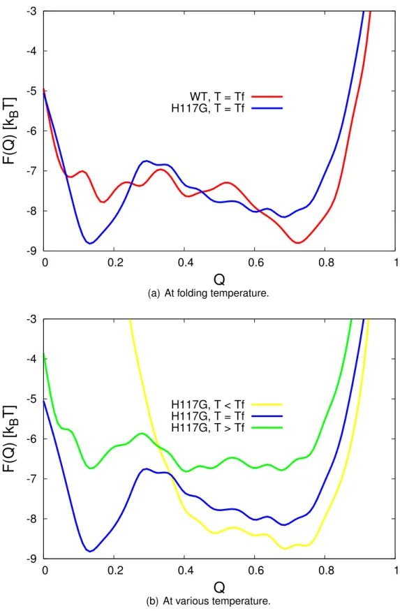
As we mentioned before, under thermodynamic conditions most of fold- ing process is known as a two state reaction. In such a case, the free energy profile has double minimum corresponding to the ensembles of native state and denatured state with varying degrees of ordering. In our case, all simu- lations indicate the two state reactions as shown in Figure 3.1(a). This result is in agreement with the experimental measurements where both of the wild- type and H117G azurins unfold in two-state without intermediates [43].

Furthermore, the three ensemble of states based on the ranges of Q- scores can be identified by this profile. The denatured state is determined by the well curve which is close to zero, in this case we have Q

Conversely, the native state is determined by the well curve near the position

where the folded state appears around Q

which is defined by the position of the free energy barrier in the Q

-9 -8 -7 -6 -5 -4 -3

0 0.2 0.4 0.6 0.8 1

F(Q) [k

T]

Q

WT, T = Tf H117G, T = Tf

(a) At folding temperature.

-9 -8 -7 -6 -5 -4 -3

0 0.2 0.4 0.6 0.8 1

F(Q) [k

T]

Q

H117G, T < Tf H117G, T = Tf H117G, T > Tf

(b) At various temperature.

Figure 3.1: Free energy as a function of reaction coordinate Q. Comparison

between mutated azurin and wild-type (a) shows a significant difference on

its double well minimum. Meanwhile, (b) shows the dependence on the

temperature where the simulation were done at T

T

, T

T

, and

T

T

, respectively.

Figure 3.1(a) also shows that the mutation of H117G gives changes in the stability of unfolding azurin. Since Q

is getting closer to zero, the mu- tated azurin gains more stability in the denatured state and less similar- ity with the native state. The lower F

at denatured state of unfolding H117G azurin shows that the unfolding of mutated azurin is faster than the wild-type azurin. In addition, at the folding temperature the mutated azurin gives sharper transition state than the wild-type. These findings obtained from free energy profile are in agreement with the experimental results [43].

As well as the mutation, temperature also affects the unfolding of azurin as shown in Figure 3.1(b). In the lower temperature (T < T

) the native state is found to be more stable. In contrast, higher temperature (T > T

) gives us broader distribution of free energy and smaller free energy barrier.

The double minimum also is not clear and its indicates that the azurin may be trapped in non-native conformation.

To observe the structural description of the unfolding process of azurin, the unfolding pathways were quantified using

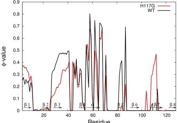
residue was calculated by using equation (3.7). The result in Figure 3.2 shows that the helix region, which contains mainly local interactions, is the most native-like compared to other regions in both wild-type and mutated azurin, as expected. The helix is found to fold faster than strands because its structure contains mainly local interactions [50]. Figure 3.2 also gives us more detailed information related to our findings from the free energy profile.

In agreement with the free energy profile, the mutated azurin unfolds faster,

specifically at β3 and β5, yet remains more native-like at β7 compared to the

wild-type. Here β3, β5, and β7 are the positions of β-strands of azurin (see

Figure 2.3).

0 0.1 0.2 0.3 0.4 0.5 0.6 0.7 0.8 0.9

20 40 60 80 100 120

φ -value

Residue

β 1 β 2 β 3 β 4 α β 5 β 6 β 7 β 8

H117G WT

Figure 3.2: Comparison of

and wild-type azurin at T

T

.

Moreover, we also compare our result with the experimental data. From our mutated azurin unfolding simulation at folding transition temperature, the average

[51] or

[52], and also with the theoretical data which is

[51]. This mutation of His117 to Gly is found to give more stability to its nearby region, β7, even though the mutated residue actually has almost no native contact with other residues. It means the non-native interaction also plays a role in our case.

3.5 Conclusion

Advancing computational study of protein folding is a great issue in bio- molecular study. Based on two fundamental theories of principle of minimal frustration and energy landscape theory, we have performed the structure- based simulation of wild-type and mutated azurin. Present study shows that the mutation of His117 to Gly affects the stability of the denatured state.

Both free energy profile and protein engineering method,

firmed that the mutated azurin folds faster than the wild-type. In particular, the β7 region, which is near the mutated residue, is found to be more stable compare to the wild-type. Nevertheless, in both types of azurin, the helix re- gion which contains more local interactions has become the most native-like region at the transition state.

In short, our findings have found to be in agreement with both experi- mental and theoretical studies. Even so, currently we only use single or- der parameter Q, defined as the measure of nativeness, to characterize the changes in free energy and observe the native and denatured states.

Further analysis may be needed to gain insights into the folding/unfolding

mechanism of azurin.

Chapter 4

Implementation of G ¯ o Model on Azurin Complex System

Previously we have applied G ¯o model on single chain of azurin via coarse- grained simulation. In this chapter, we will discuss the implementation of G ¯o model on multiple chains of azurin.

4.1 Introduction

Proteins play extremely important roles not only in human but also in other living organisms. They usually form complex interactions with other macromolecules, such as lipids, nucleic acids, or other proteins, to perform their biological functions [53]. In the last decades, this intermolecular inter- action has become a great issue in the biophysics field. Other studies have conducted to advance the computational study on intermolecular interac- tion [23, 31, 54–56].

In our present study, we will focus on protein–protein interaction. Several

studies have found that the formation of protein complex is affected by the

presence of other proteins [31, 56]. Their interactions will tend to force the

proteins to form compact configuration [57]. On the study of folding process,

G ¯o has found that the long-range interactions play an important contribution

on the stability of native conformation [21]. Inspired by his study, we predict

that the long range interaction formed by the intermolecular interaction also contributes to the conformational stability of the protein.

Here, our goal is to investigate the effects of protein–protein interaction on the conformational stability of protein complex. We developed a topology- based coarse-grained model to simulate several identical chains of azurin.

In previous chapter, we have applied G ¯o-like model to simulate single chain of azurin. This model employed the principle of minimal frustration and the funneled energy landscape. In the similar way, we will treat the intermole- cular interaction as we have treated the non-bonded interaction on the in- tramolecular interaction describing in chapter 3. These studies will provide important insights into the importance of native contacts into the stability of protein complexes.

4.2 Material and simulation methods

4.2.1 Model system

In this chapter, the native structure of azurin complex system was ob- tained from X-ray crystal structure of Pseudomonas Aeruginosa azurin (PDB ID: 4AZU) [15]. This crystal structure is composed of a tetramer of identical azurin molecules. Using this conformation, we build several systems con- sisting of dimer, trimer, and tetramer of azurin as shown in Figure 4.1. The blue chain is chosen as the representative chain that will be our focus in this observation. Meanwhile other chains act as the crowding agents.

Two dimer systems are presented here, dimer I and dimer II. Dimer I is

an independent system where the distance between the dimer is more than

the cutoff. Otherwise, dimer II is the interacted system obtained from the

original crystal structure. We add one more chain in trimer system and two

more chains in tetramer system. Both systems are also obtained from the

crystal structure, so that the tetramer system actually is the unit cell of the

crystal structure.

(a) Dimer system I

(b) Dimer system II

(c) Trimer system (d) Tetramer system

Figure 4.1: Initial configurations.

4.2.2 Potential model

We performed CG simulation with an implementation of native-structure based potential interaction to observe the dynamics of each configuration system. Our potential interaction is distinguished into intramolecular and in- termolecular interactions. The off-lattice G ¯o-like model is employed using the same formula as in Table 3.2 to represent the intramolecular interac- tions. For the intermolecular interaction energy, we adopt the non-bonded term from G ¯o-like potential in Table 3.2 which can be written in the following formula:

E

ij (r) =

ε

5

σ r

12

−6

σ r

10

+

ε

C

r

. (4.1)

To avoid the ambiguity, we introduce the superscript

to distinguish the non-bonded interaction in intramolecular and intermolecular interactions.

This indicator denotes the different chain. So, in Eq. (4.1), i and j represent i-th and j-th G ¯o particles of chain α and β respectively. Meanwhile in Table 3.2, i and j represent i-th and j -th G ¯o particles of unsubsequent particles in the same chain.

4.2.3 Simulation condition

As we have done in the non-bonded potential shown in Table 3.2, σ is set to be the reference pairwise distance obtained from the crystal structure.

The same definition of native and non-native contact is also applied. By us-

ing this potential model, we simulate all systems with the same potential

parameters and simulation condition as in the previous chapter. In addi-

tion, we avoid the translational and rotational movement of the system by

setting the momentum and angular momentum of the whole system to zero

during the simulation [58, 59] for every several steps. Our CG simulations

were performed under constant temperature on the folding temperature as

in Chapter 3.

4.3 Analysis methods

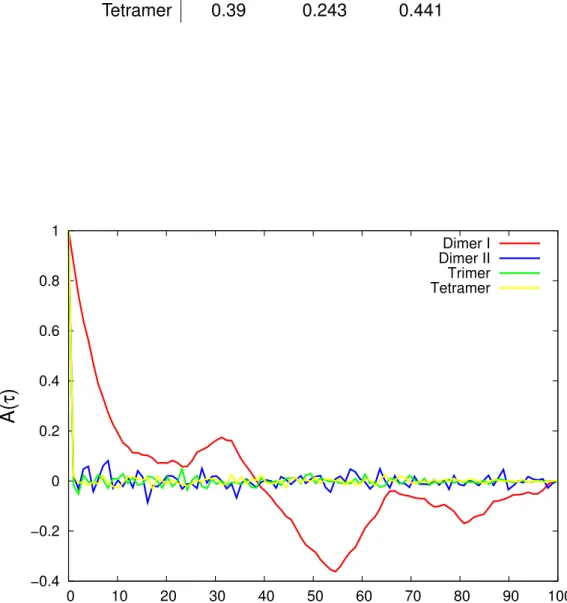
We calculated several properties to investigate the roles of the intermo- lecular interactions. We monitored the interchain dynamics by the autocor- relation of the distance between the centers of mass of pair-chains. Auto- correlation is a correlation between a time series with itself, so in our case this property can give us information whether the system remains in the same state from time to time. The autocorrelation can be calculated by the sufficient statistical average of the time series, as follows:

A(t

t

hx(t)− hxii²

, (4.2) where x is the time series property and t

is the time lag.

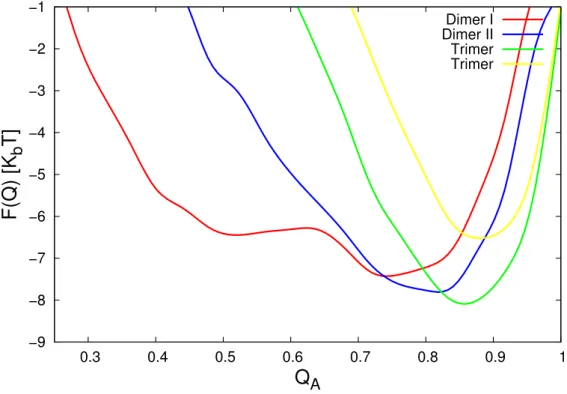
As our previous study in Chapter 3, we also compare the thermodynami- cal property using the free energy profile. The same method was used in this study, where the free energy profile is obtained by the histogram method [46]

with the fraction of nativeness (Q) as the reaction coordinate.

4.4 Results

Each system was simulated at the residue level under constant folding temperature T

. For our convenience, we will focus on two representative chains, called A and B, and compare their dynamics in all systems. Their interchain distances (d

) can be seen in Figure 4.2. These distances re- present the distance between the centers of mass of those chains.

Figure 4.2 shows that the interchain distance of dimer system I which

has no intermolecular interaction is more fluctuating than the other dimer

systems. In the dimer system I, the non-bonded interaction only involves the

non-native interaction which is a repulsive interaction, since in this system

the dimer does not have native contact. So when the dimer becomes closer,

it tends to repel and move away. On the other hand, the dimer system II

which has native contacts is much more stable. It shows that native contact plays a significant role on the interchain interaction. Besides, the crystal structure is believed to be the most stable conformation of the system.

Furthermore, the stability is also affected by the crowding system. If we compare the dimer system II, trimer system, and tetramer system which are all taken from the crystal structure, Figure 4.2 shows that the interchain distance becomes less fluctuating as the system becomes more crowded.

This comparison clearly shows the importance of native contacts on the dy- namics of protein complex as well as our comparison of the dimer systems.

The standard deviation in Table 4.1 also confirms that the system with higher compactness has smaller deviation and reaches equilibrium time faster as shown in Figure 4.3.

−30

−20

−10 0 10 20 30

0 20 40 60 80 100

d

(t)−d

(0) (Å)

Time (ns)

Dimer I Dimer II Trimer Tetramer

Figure 4.2: Time series of the interchain distances.

Table 4.1: Standard deviation of the interchain distances System chain A-B chain A-C chain A-D

Dimer I 11.448 - -

Dimer II 0.944 - -

Trimer 0.492 0.329 -

Tetramer 0.39 0.243 0.441

−0.4

−0.2 0 0.2 0.4 0.6 0.8 1

0 10 20 30 40 50 60 70 80 90 100

A( τ )

τ (ns)

Dimer I Dimer II Trimer Tetramer

Figure 4.3: Autocorrelation of the interchain distance as a function of time

lag (τ ).

−9

−8

−7

−6

−5

−4

−3

−2

−1

0.3 0.4 0.5 0.6 0.7 0.8 0.9 1

F(Q) [K

T]

Q

Dimer I Dimer II Trimer Trimer

Figure 4.4: Free energy profile as a function of reaction coordinate Q which

is the measurement of the nativeness.

Moreover, we also investigated the conformational change to see how the crowding affects the structure of individual chain. As in previous chapter, we obtained the free energy profile by using the nativeness measurement (Q) as the reaction coordinate. This free energy profile is shown in Figure 4.4. The tetramer system is found to be the most native-like configuration.

It is very natural since in the more crowded or more compact system, each residue will have less space to move, so they tend to keep the optimal dis- tance.

From the viewpoint of the potential model, the systems will tend to keep as nearly as possible to the native structure because G ¯o-like potential model minimizes the topological frustration. Nevertheless, it means that this model is very dependent to the native structure. So when the native structure do not have native contact, as in dimer system I, the system will not have the attractive interaction. Meanwhile in the real system, when they become closer and reach the contact distance, the attractive interaction exists.

4.5 Conclusions

We found that the native contact plays an important role on the dynamics of the protein complex system. Our studies also found that more crowded and compact system affects the protein movement as well. In consequence, the tetramer system which is the unit cell of the crystal structure, naturally has the most stable and native-like configuration over other systems.

G ¯o-like model can be used to reproduce the native crystal structure very

well. However, we have to consider the dependence of current intermo-

lecular potential model to the presence of native structure. More general

potential model might be considered to represent more realistic interaction

when we start from an independent system.

Chapter 5

The Effects of Intermolecular Interactions to The

Conformational Changes of Azurin Complex

In the following sections, we employ widely used Lennard-Jones poten- tial for intermolecular interaction and investigate the conformational changes of azurin complex.

5.1 Introduction

Most proteins perform their biological function by associating to form protein complex. This association involves the protein–protein interaction.

Recent studies show that noncovalent binding can influence the protein sta- bility [21, 60]. Therefore, advancing study of protein–protein interactions becomes very important for better understanding of protein function.

From the viewpoints of coarse-grained simulation, determining the protein–

protein interactions is still a great mystery. Many studies have modeled the

intermolecular interactions in protein complexes [31,56,61]. Each model has

the advantages and disadvantages depending on the goal of their studies.

In the previous chapter we have shown that non-bonded potential adopted from the G ¯o-like model gives good result to reproduce the native conforma- tion by assuming that the crystal structure is the native structure. Never- theless, the dependence on the native structure restrict us for more general implementation, such as for a larger system than the native structure. Here, we will apply more general intermolecular potential and investigate the con- formational changes of azurin complex. We treat each chain as rigid as pos- sible by employing the off lattice G ¯o-like model to represent the bonded and non-bonded intramolecular interactions [21,22]. Meanwhile the intermolecu- lar interaction is represented by the 6-12 Lennard-Jones (LJ) potential with general parameters [62]. We will observe the stability of azurin complex by analyzing the conformational change and total surface area.

5.2 Material and simulation methods

5.2.1 Model systems

As in the previous chapter, currently we build several systems consisting of dimer, trimer, and tetramer of identical azurin as shown in Figure 5.1.

System I, IV, and V are taken from the original crystal structure (4AZU).

System II and III are modified dimer systems which have intermolecular

interaction with different contact areas.

Figure 5.1: Various initial conformations. System I, II, and III are dimer

systems with different contact orientation.

5.2.2 Potential model

We carried out coarse-grained simulations by combining native-structure based potential interaction for the intramolecular interaction and physics- based potential for the intermolecular interaction. The same intramolecular potential will be used to minimize the topological frustration of each chain, since we will focus more on the protein–protein interaction. The widely used 6-12 Lennard-Jones potential will be applied as the intermolecular interac- tion to describes the van der Waals term [62, 63]. This potential is defined as follows:

U

σ

r

−

σ r

6

, (5.1)

where r represents the pairwise distance between two residues from differ- ent chains and σ is the distance where the intermolecular potential between two residues is zero.

5.2.3 Simulation condition

In current study, we redefine the units for our coarse-grained model using the same quantities as our previous units, which are length (σ

), mass (m), time (τ ), and energy (ε

). The values of our new coarse-grained units are listed in Table 5.1. The values of σ

, m, and ε

are determined from the average van der Waals radii of azurin, the average mass of azurin, and the temperature of system, respectively. The time unit (τ) is calculated by the same method as in Chapter 3. We also redefine the potential parameter and simulation condition as in Table 5.2.

Table 5.1: New units of coarse-grained model CG units Experimental units

length σ

5.7 Å

mass m 110 amu

energy ε

0.6 kcal/mol

time τ 3 ps

Table 5.2: Potential parameter and simulation condition Parameter Value in kcal/mol Virtual bond-stretching K

Å

Virtual bond-angle bending K

Virtual bond-torsional term K

Native ε

Non-native ε

Intermolecular ε

or

Others Value

LJ distance σ

Å

Friction coefficient ζ

(τ

)

Temperature T

K

For the estimation of σ and ε

for intermolecular interaction, we con- sider the correlation with the non-bonded potential model for intramolecu- lar interactions as shown in Table 5.3. It is not easy to clearly obtain the value of those parameters. The r

on intramolecular interaction represents specific distance obtained from the crystal structure where each pair has different value. Meanwhile σ, set as general parameter for all pairs, usually represents the particle size. Here we use σ

Å, because the interact- ing residues within

Å is found to contribute significantly to the protein–

protein association [61]. By comparing the minimum value of the potential, ε

should be smaller than ε

since intermolecular interaction is weaker than the intramolecular interaction.

Table 5.3: Comparison of two non-bonded potential Intramolecular Intermolecular 10-12 LJ potential 6-12 LJ potential Potential (U

ε

5 ^r_r⁰12

−6 ^r_r⁰10i

4ε_LJh

σ r

12

− ^σ_r6i

U

r

5/6r₀

r

σ

Minimum U

when r

r

when r

σ

U

U

σ) =

5.3 Analysis methods

We measured the structural stability of azurin complex through the root mean square displacement (RMSD) with respect to the initial structure. A least-square fitting on given structure to the initial structure is performed to obtain minimal RMSD. We also analyzed the total surface area of the system to gain insight into the accesibility of the system to a solvent. This concept was first introduced by Lee and Richards [64]. Our calculation applied sta- tistical approach for faster calculation of accesible surface area, proposed by Wodak and Janin [65], and was performed by using POPS program [66].

5.4 Results

In this section we will explain our analyses into two part. First, we inves- tigate the effects of intermolecular interaction strength to the stability of the system. We will compare two parameter values of ε

as in Table 5.2 for the simulation of system I. Later, we found that ε

kcal/mol is better and we will use it to simulate the other systems. Second, we evaluate physical properties for all systems as described in previous section.

Higher intermolecular potential parameter represents stronger interac-

tion, so we expect that two chains will tend to get closer and the buried area

will increase. Our expectation is well confirmed as shown in Figure 5.2. This

figure shows that the conformation of both chains are starting to denature

as indicated by the steady increment of RMSD values of both chains. This

denaturation is appropriate with the aggregation possibility that is shown by

the decrease of total surface area (Figure 5.3). On the other hand, Figure

5.4(a) shows that the simulation with smaller ε

gave more stable confor-

mation. These findings show that strong attractive interaction may lead the

system to aggregation.

0 1 2 3 4 5 6 7 8

0 50 100 150 200 250 300

RMSD (Å)

Time (ns)

chain A chain B

Figure 5.2: The root mean square displacement shows the conformational changes compared to the given initial configuration caused by the strong intermolecular interaction.

0.7 0.8 0.9 1

0 50 100 150 200 250 300

Normalized SASA

Time (ns)

Figure 5.3: The total surface area is calculated at the residue level and is

normalized by the total surface area of independent chains where the actual

surface area of one chain is 6735.87 Å

.

0 1 2 3 4

0 50 100 150 200 250 300

RMSD (Å)

Time (ns)

chain A chain B

(a) System I

0 1 2 3 4

0 50 100 150 200 250 300

RMSD (Å)

Time (ns)

chain A chain B

(b) System II

0 1 2 3 4

0 50 100 150 200 250 300

RMSD (Å)

Time (ns)

chain A chain B

(c) System III

0 1 2 3 4

0 50 100 150 200 250 300

RMSD (Å)

Time (ns)

chain A chain B chain C

(d) System IV

0 1 2 3 4 5 6

0 50 100 150 200 250 300

RMSD (Å)

Time (ns)

chain A chain B chain C chain D

(e) System V

Figure 5.4: The root mean square displacement of the simulations with

ε

kcal/mol.

Table 5.4: Quantitative comparison of the RMSD of each system is rep- resented by the calculation of average (Å) and standard deviation (Å) of RMSD.

System Average(Standard deviation)

Chain A Chain B Chain C Chain D

I 1.84(0.28) 2.15(0.37) - -

II 1.88(0.30) 1.94(0.30) - -

III 2.11(0.44) 2.35(0.50) - -

IV 2.17(0.45) 1.91(0.34) 1.77(0.28) - V 1.98(0.34) 2.68(0.76) 1.87(0.35) 2.46(0.74)

Table 5.5: Comparison of the initial and average surface area (Å

), initial number of pair contacts, and average total energy (kcal/mol).

System Total SASA (Å

) initial Av. total Initial Average #contacts energy

I 12982.76 13750.75 13 125.99

II 13178.79 14186.64 8 131.03

III 12897.96 13827.58 19 126.78

IV 18615.81 19931.83 35 164.86

V 24108.12 25705.4 82 211.12

Now let us investigate the dynamics of azurin complex regarding to the role of initial contacts. We measure the structural stability of each chain from the given configuration against the initial state and compare the behavior of all systems as shown in Figure 5.4. Figure 5.4 shows that the conforma- tions of azurin remain relatively stable at all systems. This finding is also confirmed quantitatively in Table 5.4. The averages of RMSD are below 3 Å with relatively small deviation.

We also monitor the total surface area (SASA) of azurin complex at residue level. By this calculation we can investigate the buried area in the binding site. From our calculation, the total surface area of all system in- creases about 1,000 Å

(see Table 5.5). Meanwhile, Figure 5.5 shows that the ratio of total SASA of the azurin complex to total SASA of independent chains decreases. This decrease represents the increase of buried area, which indicates the strong attractive interaction in the binding site.

Moreover, Figure 5.6 shows that the ratio of SASA decreases along with