July25,2017GraduateSchoolofInformationScienceTohokuUniversity RanWensheng Master’sThesisModelingRelationshipsbetweenObjectsforReferringExpressionComprehension B5IM2503

B5IM2503

Master’s Thesis

Modeling Relationships between Objects for Referring Expression Comprehension

Ran Wensheng

July 25, 2017

Graduate School of Information Science

Tohoku University

A Master’s Thesis

submitted to System Information Sciences, Graduate School of Information Science,

Tohoku University

in partial fulfillment of the requirements for the degree of MASTER of ENGINEERING

Ran Wensheng Thesis Committee:

Professor Kentaro Inui (Supervisor) Professor Takayuki Okatani

Professor Yoshifumi Kitamura

Associate Professor Okazaki Naoaki (Co-supervisor)

Modeling Relationships between Objects for Referring Expression Comprehension ^∗

Ran Wensheng

Abstract

The Referring Expression Comprehension (REC) task is to correctly identify an object in an image that corresponds to a given natural language expression (i.e., referring expression). In this thesis, we improve a previous REC model by explicitly aligning relations between mentions in a language expression to pairs of objects placed in specific relative positions in an image. Evaluation using the Google Refexp dataset [1]

demonstrates that the proposed model outperforms the baseline method. In addition, we found that in stead of the image features extracted from a pretrained convolution neural network and popularly used by previous research, one can simply boost performance by using automatically recognized category labels.

Keywords:

Neural Network, Convolutional Neural Network,word2vec,Bipartite Graph, Referring Expression

∗

Master’s Thesis, System Information Sciences, Graduate School of Information Sciences, Tohoku

University, B5IM2503, July 25, 2017.

∗

Contents

1 Introduction 1

2 Related Work 3

3 Background 5

3.1 Machine Learning and Neural Network . . . . 5

3.2 Recurrent Neural Network . . . . 9

3.3 Convolutional Neural Network . . . . 11

4 The Proposed Model 14 4.1 Constructing the Bipartite Graph . . . . 14

4.2 Learning . . . . 17

5 Experiment 19 5.1 Dataset . . . . 19

5.2 Evaluation Metrics . . . . 19

5.3 Implementation Details . . . . 19

5.4 Results and Analysis . . . . 20

5.4.1 Analysis on Subsets of Validation Data . . . . 20

∗

, B5IM2503, 2017 7 25 .

5.4.2 Instance Analysis . . . . 21

5.5 CNN Vector or Category Label as Visual Features? . . . . 23

5.6 Faster RCNN Vector as Visual Features . . . . 24

5.7 Comparison with Related Work . . . . 25

6 Conclusion and Future Work 26

Acknowledgements 27

List of Figures

1 Referring expression: the desk with beer on it. There are two desks in

the image.(This image comes from MSCOCO dataset [2].) . . . . 1

2 The proposed method. . . . . 4

3 A neuron . . . . 7

4 Neural Network . . . . 8

5 A Recurrent Neural Network Language Model. The word predicted in time step t is calculated from current internal state, which is expected to encode all the information seen before. . . . 10

6 A illustration of the convolution layer. . . . 12

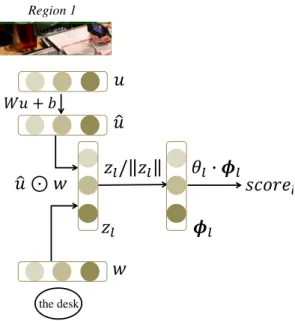
7 Local score calculated for an edge (region 1, the desk). Here, θ

, W , b are the model parameters, w is the average of the word vectors in the NP, and u is the visual representation of the object in the image. . . . 16

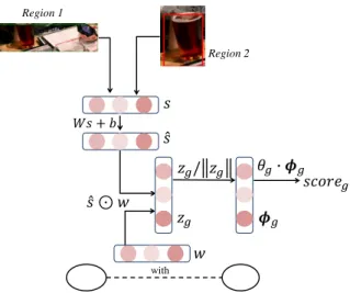
8 Global score calculated for (with, region 1, region 2). Here, θ

, W , b are the model parameters, w is the average of the word vectors in the relationship phrase, and s is the spatial information of the bounding boxes of two objects. . . . 17

9 Examples where the proposed model improves the baseline. . . . . . 22

10 An error made by the proposed model. . . . 22

11 An error made by both the baseline and proposed models. . . . 23

12 An example showing that the one-hot category vector is more helpful

than the VGG vector. . . . 24

List of Tables

1 Performance of baseline and proposed models on the validation set. . 20 2 Accuracies on subsets of training (Set A) and validation (Set B) data. . 21 3 Accuracies with different visual representations on the validation set. . 23 4 Accuracies with different visual representations on the validation set. . 24 5 Accuracies evaluated on ground truth bounding boxes in the validation

set. . . . 25

1 Introduction

We use referring expressions in daily conversation to indicate which person or object we are identifying, such as “the man on the left” and “the girl dressed in blue”. There are many objects in the image shown in Figure 1, such as a beer, two desks, and a woman.

The expression the desk with beer on it can unambiguously indicate the referenced object. We call a phrase that indicates the object bounded by the green box a referring expression.

desk

beer desk

Figure 1: Referring expression: the desk with beer on it. There are two desks in the image.(This image comes from MSCOCO dataset [2].)

The task to identify a region from a given referring expression is called Referring Expression Comprehension (REC) [1]. In this thesis, we propose an algorithm to solve the REC task. Making computers understand referring expressions has applications in human-computer interaction, such as enabling robot-human interactions in the physical world. Resolving referring expressions requires understanding of natural language and perceiving the rich visual world around us, which is a long-standing goal of artificial intelligence. We must develop models and techniques that allow us to connect the visual data domain and the natural language domain, to perform translations between these domains.

Referring expressions often contain various information, such as attributes and relations with other objects that are necessary to identify the target object in the image.

The example in Figure 1 illustrates the need for relation information to resolve the REC

task. Here, suppose we want to localize the object desk referenced by the referring expression. If we do not consider the relationship between the desk entity and the beer entity, we cannot ground the referring expression because there are two desks in the image.

Previous studies have either ignored the relation information between objects or modeled this relationship in an implicit manner. In these approaches, the referring expression is embedded as a vector generated from a language model conditioned on an image representation. Even if more than one entity is mentioned in the phrase, the relationship is not modeled explicitly because the phrase is represented by a single vector.

In this thesis, we incorporate relation information explicitly by mapping relationships between entities in a referring expression to the spatial relations between corresponding objects in an image. Specifically, we first extract entities from the referring expression and objects from the image. Then, we learn an alignment between entities and objects.

In this alignment, relationships between entities and the relative positions of objects are considered explicitly. For example, from the image shown in Figure 1, we can extract two entities from the referring expression (i.e., desk and beer) and three objects from the image. The relation “with” between these two entities is paired with the positions of any two objects in the image to calculate a score, which models the appropriateness of the alignment.

We evaluated our model using the Google Refexp dataset [1] to demonstrate that

the proposed method outperforms a baseline (Section 5.4). Moreover, our analysis

indicates that taking relationships into account is crucial for the performance gain

(Section 5.4.1,5.4.2). In addition, the analysis leads to a surprising discovery that one

can boost the performance of REC simply by replacing a widely used convolution neural

network feature with automatically recognized category labels for visual representation

(Section 5.5).

2 Related Work

REC is a classic Natural Language Processing (NLP) problem [3]. Before deep learning methods became widely used in the NLP field, most studies focused on relatively small datasets of artificial objects, and the text comprehension and vision modules were separate processes. Traditional approaches understand referring expression by enumerating attributes (size, color, etc.) or predefined relationships explicitly; thus, they could not flexibly handle abundant real-world natural expressions. [1] were the first to apply deep learning methods to REC and they released a large dataset. In this study, we evaluate on the dataset and compare to [1]’s baseline. The baseline uses a Convolution Neural Network (CNN) to extract feature vectors from candidate regions, then feeds the vectors to a Long Short-Term Memory (LSTM) language model and calculates the generating probabilities as scores. However, [1] do not consider the target object’s relationships with other objects in the image. Especially when there are multiple objects of the same type presented in the image, it is often insufficient to distinguish the target object from other objects of the same type by encoding only the object’s attribute information but ignoring relations between objects, as shown in the example in Figure 1.

[4] and [5] attempted to encode relation information into the visual representation of objects. Specifically, in the method proposed by [4], the input CNN features are obtained from a (region, context-region) pair where the whole image together with other objects in the image is considered a context region. Such a feature vector may implicitly encode relations between the target object and other objects. [5] employ a more focused approach to encode context information. In addition to CNN features, they add object comparison features to the visual representation, which is taken as the difference between the vectors of the target object and other objects. Both approaches consider relations in an implicit manner. [6] model relationship explicitly, but only one relation is considered for each referring expression. Our proposed model has the ability to handle multiple relations, and we compare our method with the above works in Section 5.7.

Related to REC, there are other image understanding tasks attempting to ground

natural language expressions to images in a fine-grained manner. For example, [7] and

[8] learn alignments between regions in an image and fragments in a natural language

expression, which is used for the image retrieval task. [9], [10], and [11] are approaches

Clip out objects from image

The desk with

beer on it. with

the desk beer

One possible alignment

Parse to extract NP and relationship

Region 1

Region 2

Region 3

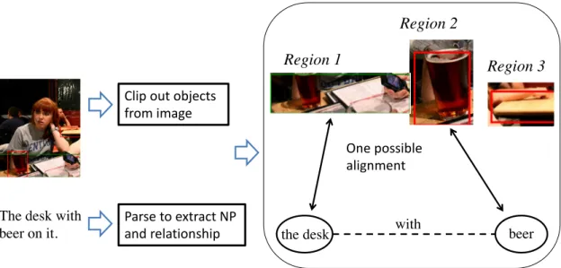
Figure 2: The proposed method.

for relation extraction from an image. Joint learning with these models will be an

intriguing future direction.

3 Background

In this chapter, we introduce the basic concepts of machine learning and a subfield of machine learning - neural network, which are necessary to understand the methods proposed in following chapters,in order to make this thesis relatively self-contained.

3.1 Machine Learning and Neural Network

Self-learning is an important procedure for computers to deal with the problems that are difficult or time-consuming to approach in a conventional, rule-based manner.

For example, now we want computer to recognize the concept of animal cat. In the conventional way, we may traverse all the features related to cat in an exhausted manner, which requires plenty amounts of specific knowledge of cat and careful design of rules.

But in a machine learning way, we can collect large number of cat images and annotate them with the right tag and let the computer learn the input output relationship implied by the training data(image-tag pairs).

In machine learning, there are several subfields containing supervised learning, unsupervised learning and reinforcement learning. In supervised learning, we have training data and corresponding tags which served as a teaching signal. Contrarily, in unsupervised learning we only have training data and we have to learn the patterns or regularities from data without any tag or signal. In reinforcement learning, our goal is not to discriminate the data or model the generation mechanism o data but to solve a sequential decision making problem. In this thesis, we only use supervised learning.

There are several key elements in supervised learning. Mapping Function , Loss Function, Optimization Process, Regularization. We try to give an explanation to these

important concepts.

Actually the machine learning problems can be formulated as trying to find a mapping

f : X → Y where X is an input space and Y is an output space,by taking the advantage

of existing samples. For example, X may be the visual space of images and Y could be

a binary variable. When Y is 0, it means the cat appears somewhere in the image, and

is 1 when the input is not a cat image. And this problem can be called a classification

problem since the output Y is a categorical variable from some finite set. Common

classification problems include image classification, document classification, sentiment

analysis. If Y is real-valued scalar, then the problem is called the regression problem.

The regression technique can be used for forecasting, time series modeling.

Suppose we have N samples D={(x

, y

) where i=1,2,....,N} called training set. We want to find a mapping f that can minimize sum error over D.

ˆ

y

= f (θ

; x

) (1)

min 1 N

N

X

i=1

L(y

, y ˆ

), (2)

where L(y

, y ˆ

) is the loss function, and f is the mapping function.For classification problems, the loss function can be cross entropy loss, and for regression problem, the loss function can be mean squared error.

Note that our ultimate aim is to develop a model that can make accurate prediction over unseen data. But equation 1 only minimize the loss over seen data. That is we hope that optimizing 1 serves as a good proxy for our ultimate goal. But unfortunately sometimes it may not work. Suppose the extreme occasion that we learn the mapping f that can perfectly output values y

for each input x

in the training dataset, but output 0 for any other data which are not in the training set. For this problem we say that the model is over fitted by the training data and have no generalization ability. In order to alleviate this problem, we can introduce a regularization term in 1. That is, we now have:

min 1 N

N

X

i=1

L(y

, y ˆ

) + R(f ) (3) where R is a scalar-valued function that encodes preference for some functions over others, regardless of their fit to the training data. The regularization term can be considered as an application of Occam’s razor theory, which is stated as ”Suppose there exists two solutions for a problem, then the simpler one is usually the better one”. So the regularization term can also be considered as a measurement of the complexity of mapping f. We want to find some kinds of mapping f that not only have a reasonable prediction accuracy over training dataset but also be as simple as possible.

Now we give a brief introduction of neural network. Neural network is a network

composed of many basic elements called neuron. Fig. 3 shows a single neuron. A

Figure 3: A neuron

neuron receives an input vector x = (x

, x

, x

), and then multiply it with weights w = (w

, w

, w

). The result is summed with a variable called bias, which can be represented as z. So we have: z = P

i=1

x

∗ w

+ b. Then z is input to a non- linearity function g(also known as activation function), so finally we get the output a = g(z) = g( P

i=1

x

∗w

+b). Note that commonly used activation function is sigmoid function f(x) =

, tanh function f(x) =

1+exp(2∗x)

and the rectified linear

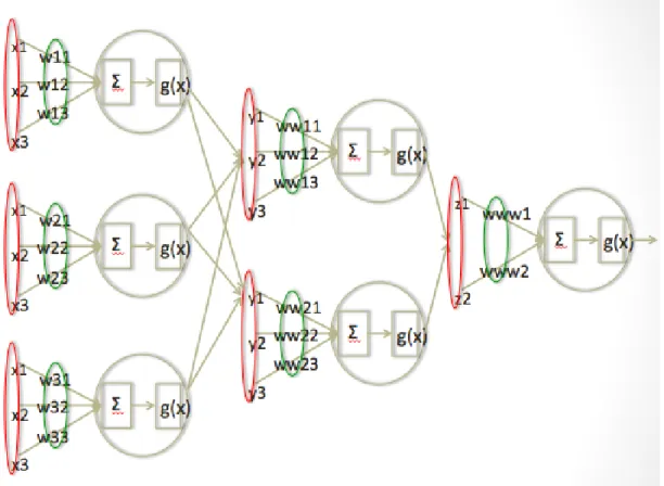
unit(ReLU) f (x) = max(0, x). A neural network (shown in Figure 4) is composed of

many neurons stacked horizontally(next to each other) and vertically(on top of each

other) and is followed by a final output layer. If there are several layers in a network,

for a specific layer i, it receives input from previous layer, x

= a

, then compute the

activation a

and pass it to the next layer. For a binary classification problem, the final

neuron output a real-valued scalar p,taking value from 0 to 1, which can be interpreted

as probability to a specific category, say class 1. If p is larger than 0.5, then model

output prefers to class 1 with respect to input, or if p is smaller than 0.5, the model

chooses class 2.

Figure 4: Neural Network

Now that we already defined the computation flow of a network, now we have to teach the supervised signal to the neural network so that it can know how to adjust the parameter to give better predictions for training data. We use cross entropy loss as the loss function for classification problem.

L(D; θ) = 1 N

N

X

i=1

−y

log ˆ y

− (1 − y

) log (1 − y ˆ

) (4) where y ˆ

is the output of neural network, y ˆ

∈ (0, 1) and y

is the label for sample x

, which is either 0 or 1.Since the likelihood of the data D given parameter is

P (y

= 1|x

; θ) = ˆ y

∗ (1 − y ˆ

)

(5) Likelihood(D; θ) =

N

Y

i=1

P (y

= 1|x

; θ) (6)

the negative log likelihood of equation 6 can be written in equation 4. In order to minimize the equation 4, we can compute the gradient can then adjust parameters along the gradient direction. We iterate this process until the function converge to a locally optimum.This is called the gradient descent algorithm.

θ

= θ

− α ∂L(D; θ)

∂θ |θ = θ

where α is a small positive scalar called the learning rate. As for computing the gradient of the neural network, we refer to read papers about back propagation.

3.2 Recurrent Neural Network

The Recurrent Neural Network(RNN) is a variant of the neural network which can process sequential data by taking the output h

of itself at time step t − 1 as input at time step t. More specifically, we have formula h

= f

(h

, x

), where f is the function depending on the kind of network architecture. and h

is the internal state of model that encodes the information of the history. Every time the model receives a new input x

, it updates the internal state h

using the formula above. The parameter θ is reused every time step, allowing model to deal with sequences with arbitrary lengths.

For vanilla RNN architecture, we have

h

= tanh(W

x

+ W

h

)

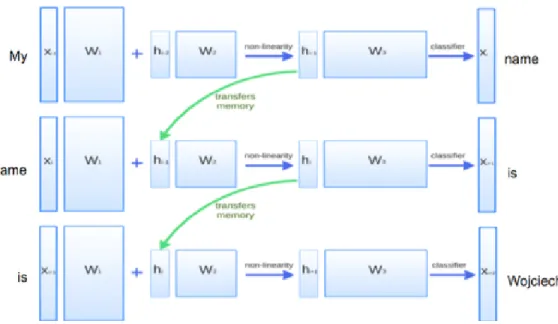
and the tanh nonlinearity can also be replaced with ReLU. A classical application of RNN is the recurrent neural network language model as illustrated in Figure 5. A language model is a probabilistic model of a sequence x

, x

, ...., x

.

p(x

, x

, ..., x

) =

n

Y

i=1

p(x

|x

) (7)

The probability p(x

|x

) is calculated by linearly transforming the current internal state into a probability distribution over all words in the vocabulary.

p(x

|x

) = softmax(W

h

)

The parameters W

, W

, W

are learned by maximizing the equation 7 using cross

entropy loss.

Figure 5: A Recurrent Neural Network Language Model. The word predicted in time step t is calculated from current internal state, which is expected to encode all the information seen before.

The vanilla RNN suffers from the problem of exploding gradients and vanishing gradients which can be alleviated by Long Short Term Memory(LSTM). In LSTM, the input h

and x

are computed in a more complex manner and besides the internal state h

, LSTM also introduce memory cell c

to store the long-period information. Each time the LSTM can decide to overwrite a memory cell, retrieve the content from it, or keep its contents for the next time step by using explicit gating mechanisms. The precise form of the update of h

and c

is as follows:









 i f o g











=









 sigm sigm sigm tanh











W x

h

!

c

= f c

+ i g

h

= o tanh(c

)

Recently, the RNN is widely applied in sequence to sequence problems [12] such as machine translation [13], caption generation [14] and so on. Actually, the RNN can also be used as a sentence or phrase encoder that compress the semantic meaning into real-valued vectors.

3.3 Convolutional Neural Network

In fully connected neural network, the node in layer i is connected to each node in layer i − 1. But in convolutional neural network, the node in layer i is only connected to a part of nodes in layer i − 1, which is different from the common linear layer. This specially designed architecture is convenient in handling data with spatial topology.(e.g, images, videos, character sequence in text) and is called convolution layer. As the pixels in image data are only correlated with nearby pixel, a node in the upper layer only need to connect a part of the node in the lower layer and the connection weight can also be shared with all other nodes in the same upper layer.

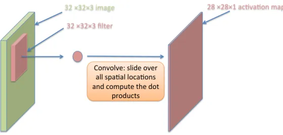
In Figure 6, we can see that a node in upper layer(activation map in the figure) is computed from a 5*5-sized subregion in original image. By sliding a fixed-size filter along the horizontal and vertical direction we can get many nodes in the upper layer as each node is corresponding to a different position for the filter. Weights used to computed the node in activation map is the same when filter slides in different position.

Intuitively, the filters has capacity to look for certain local features in the input layer.

Local connectivity and parameter sharing property of Convolutional Neural Network can reduce the parameter in each layer , thus allows us to stack several layer or even hundreds of layers to build a complex architecture [15].

Besides convolution layer, it is also common to use pooling layer in the convolutional

network architecture. The pooling layer is a kind of down-sampling method that

can reduce the input data by a fixed factor. A widely used pooling layer is 2*2 max

pooling layer with stride 2. That is we have a 2*2 sized filter sliding in the input tensor

horizontally and vertically with a step size of 2. For each position of filter, it receives

4 inputs and returns the maximum value. Then the filter slides to the next position

with step size of 2, making the neighbor positions not overlap with each other. So the

size of input tensor is reduced by a factor of 4, at the cost of losing some local spatial

32 ×32×3 image 32 ×32×3 filter

28 ×28×1 ac1va1on map

Convolve: slide over all spa1al loca1ons and compute the dot

products

Figure 6: A illustration of the convolution layer.

information.

A convolutional network is composed of convolution layer, fully connected layer(the common linear layer),pooling layer and RELU layer. The ConvNet is used in image classification. We input an image to the network and adjust the parameter of convolution layer and fully connected layer so that the network can output the right category of the input.

By analyzing the convolution network trained on large scale image dataset we ob-

serve that the lower layer in convnet captures the local information of input image such

as texture, lines and shapes, while the high layer captures more abstract information

such as the content of input. Therefore, once trained on large-scale image dataset

such as [16] for image classification task , we can say that the network along with the

learned parameters are able to extract useful information from a given image. Extracted

information from images are in the form of vectors and are called the representation

of images. More specifically, we have v = CN N

(I) , where CNN is a well-designed

ConvNet with pre-trained parameters θ, I is the input image pixels, v can be the vector

of the layer right before the softmax layer. There are some famous network architectures

whose model parameters are public to use such as AlexNet [17] and VGGNet [18].

4 The Proposed Model

In this chapter, we will introduce the proposed method in detail. Given an image with several objects, and a referring expression pointing to a given target object, we first parse the referring expression to extract all noun phrases (NPs) and the relationships among them. Then, an alignment between the referring expression and the image is constructed as a bipartite graph, in which NPs in the referring expression and objects in the image are considered as nodes, and the correspondences between them are represented as a configuration of edges in the graph. Given the nodes, we assign a score to each possible graph to measure how good the alignment is. We use machine learning methods to learn the parameters of the scoring function.

4.1 Constructing the Bipartite Graph

For each input pair of referring expression and candidate objects, we construct a graph and assign a scalar score Score(x, y) to the bipartite graph. We want the model to learn parameters automatically so that it can assign a high score to the correct graph and a low score to incorrect graphs. A correct graph means that all NP nodes are correctly connected to the object nodes they refer to. There are many possible graphs given an input pair; thus, the task is to search for a graph with the maximum score.

ˆ

y = arg max

y∈G(x)

Score(x, y) (8)

Here, G(x) is the set of all possible graphs given an input pair x of a referring expression and candidate objects. For example, as shown in Figure 2, x comprises three nodes of object regions on one side of the graph and two NP nodes on the other side. Here, y ˆ represents the correct graph and y is an arbitrary graph in G(x). Score(x, y) comprises both a local score score

and a global score score

, which are defined as follows.

Score(x, y) = X

e∈E(y)

score

(x, e) +

X

(ei,ej)∈Epair(y)

score

(x, e

, e

) (9)

score

(x, e) = θ

· φ

(x, e) (10)

score

(x, e

, e

) = θ

· φ

(x, e

, e

) (11)

Here, E(y) is the set of edges in graph y, and E

(y) is the set of pairs of edges whose NP nodes form a relationship. score

is the local score which captures how well the entity mentioned in referring expression is matched to an object in the image. score

is the global score, which measures the fitness of the textual representation between entities in the referring expression and the spatial relationship of objects in the image. θ

and θ

are the model parameters to be learned, and φ

(x, e) and φ

(x, e

, e

) represent local and global features, respectively.

For example, in Figure 2, the score of the graph is the sum of the local scores for (region 1, the desk) and (region 2, beer), together with the global score for (with, region 1, region 2).

The score for an edge (local score) or a pair of edges (global score) is calculated using the dot product of a feature vector (local or global features) with the model parameters. To compute the local score of an edge, we first extract representations for both an entity node from an NP and an object node from the bounding box in the image. Specifically, the representation of the entity node denoted as w, is calculated by averaging the embeddings of words in the NP. Here, word embeddings are initialized using the pretrained word2vec [19], which is a 300-dimensional vector representation.

For an object node denoted as v, the representation includes the visual feature extracted from object image using a pretrained VGG-16 CNN model [18]. We also incorporate the spatial information of the bounding box, denoted as s, into object representation.

Specifically, s := [

,

,

,

,

image

], where W and H are the width and height of the image from which the candidate object is obtained, and (s

, s

) and (s

, s

) are the top-left and bottom-right coordinates of the bounding box, respectively. S

is the area of the entire image and S

is the area of the region. This results in a 1005-dimensional vector u := [v, s].

After the representations for both the object node and the NP nodes are obtained, a

local feature that incorporates both textual and visual information is calculated. Note

that the dimensions for u and w differ; thus, we perform linear transformation on u

to make the dimensions of the two vectors the same. Here, we adopt the element-

multiplication method to combine representations from language and vision, following

the desk

Region 1

𝑢 𝑢"

𝑤 𝑊𝑢 + 𝑏

𝑧 ₍ 𝑢" ⊙ 𝑤

𝝓 ₍ 𝑧 ₍ / 𝑧 ₍

𝑠𝑐𝑜𝑟𝑒 ₍ 𝜃 ₍ 2 𝝓 ₍

Figure 7: Local score calculated for an edge (region 1, the desk). Here, θ

, W , b are the model parameters, w is the average of the word vectors in the NP, and u is the visual representation of the object in the image.

previous research [20]. Thus, we obtain the following formulas:

ˆ

u = W u + b (12)

z

= ˆ u w (13)

φ

= z

/||z

|| (14) where is the elementwise multiplication between two vectors. Once the local feature φ

(x, e) is calculated using Equation (7), it can be used to calculate the local score using Equation (3). Figure 7 illustrates the local score computation.

For global scores, we calculate the global feature φ

(x, e

, e

) using the spatial information of two bounding boxes, denoted as s, and the average embeddings of words in the relationship phrase, denoted as w. Thus, we have:

ˆ

s = W s + b (15)

z

= ˆ s w (16)

φ

= z

/||z

|| (17)

Finally, the global score is calculated from the global feature and model parameter using Equation (4). Figure 8 illustrates the above computation.

with

𝑠

𝑠̂

𝑤 𝑠̂ ⊙ 𝑤

𝑧

𝑧

/ 𝑧

𝝓

𝑠𝑐𝑜𝑟𝑒

𝜃

1 𝝓

Region 1

Region 2

Figure 8: Global score calculated for (with, region 1, region 2). Here, θ

, W , b are the model parameters, w is the average of the word vectors in the relationship phrase, and s is the spatial information of the bounding boxes of two objects.

4.2 Learning

In the proposed model, the parameters to be learned come from the word embeddings and the weight matrices in local and global scores. Our objective is to minimize the following function:

J(θ) = min

N

X

k=1

l

(θ) (18)

where

l

(θ) = max

gk∈_G(x)

Score(x

, g

; θ)

−Score(x

, g ˆ

; θ) + ||g

− g ˆ

||

(19)

Note that g ˆ

represents the correct graph and g

is a candidate graph. ||g

− g ˆ

||

denotes the Hamming distance between the candidate and correct graphs. N is the

total number of instances in the training set and l

(θ) is the loss for the k-th instance.

This formula makes the score for the correct graph larger than the candidate graph by a certain margin. After training, we simply choose a graph with the largest score during inference. According to this graph, the output is the object connected to the head NP of the referring expression.

In this problem setting, only the object corresponding to the head NP can be obtained as gold annotation from the training data; this means that the “correct” objects referenced by other NPs are unspecified. For example, in Figure 2 the correspondence between the head NP the desk and Region 1 can be obtained from training data, but the correct correspondence between beer and Region 2 is not given. We expect the model to learn such latent alignments automatically.

In order to achieve this, we sample alignments between objects and non-head NPs during training, with probabilities proportional to their local scores. Then, a “correct”

graph is obtained by adding the gold annotation as an edge connecting the head NP to

one object, and an incorrect graph is obtained by connecting the head NP to another

object. We maximize the margin between scores of the two graphs, which include

global scores.

5 Experiment

In this chapter, we evaluate the proposed model on the Google Refexp dataset [1] and analyze the results.

5.1 Dataset

Google Refexp is constructed on top of the MSCOCO dataset [2], which comprises images of complex everyday scenes containing common objects in natural contexts.

[1] selected images from the MSCOCO dataset that contain at least two instances of the same object type and the bounding boxes of the objects occupy at least 5% of the image. Then, they constructed an Amazon Mechanical Turk task in which each object is presented and the worker is asked to generate a unique text description for the given object. They also constructed a second task in which a different worker is asked to click the object given the referring expression generated in the first task. If the clicked object overlaps the true object, then the referring expression is considered valid and is added to the Google Refexp dataset. This resulted in a dataset of 54822 objects in 26711 images and 104560 expressions. The dataset was split into a validation set with 5000 objects, a test set with 5000 objects and a training set with the remaining objects. The the author of the Google Refexp dataset has only published training and validation sets; therefore, we report the accuracy of models on the validation set.

5.2 Evaluation Metrics

For evaluation, one calculates the Intersection over Union (IoU) ratio [1] between the bounding box of the true object and the the bounding box of the object predicted by the model. If IoU is larger than 0.5, the output is regarded as true. Accuracy is computed as the percentage of true predictions in the validation set.

5.3 Implementation Details

We used Stanford CoreNLP [21] to parse referring expressions. We use constituency

parsing to extract NPs and relation expressions are taken as dependency paths between

NPs. We used word2vec [19] to initialize embedding of all words in NPs and rela-

tion expressions. For the visual representation, we extracted CNN features from the

Methods Accuracy

[1] 42.50

Re-implementation (baseline) 40.01

Proposed model 44.01

Proposed model w/o global score 34.67

Table 1: Performance of baseline and proposed models on the validation set.

bounding box region of the object using the 16-layer VGGNet [18] pretrained using the ImageNet database [16]. We used 1000 dimensional vectors from the last layer (fc8) of VGG and fine tuned the last layer. Note that the visual feature of an object is this CNN feature concatenated with the spatial information of the bounding box (Section 3).

We implemented the proposed model using Chainer [22]. We used Adam [23] for optimization, with a learning rate of 0.01. The batch size was set to 16. We did not employ a regularizer.

5.4 Results and Analysis

Accuracy of the proposed model on the validation set is shown in Table 1. For com- parison, we re-implemented the baseline method of [1], and show its result together with the originally reported accuracy. In order to determine whether the global score component is acturally required for this task, we removed the global score from the model and evaluated the resulting model. As Table 1 demonstrates, the accuracy of our reimplementation is nearly equal to that reported by [1], and the proposed model outperforms the baseline. On the other hand, when trained without a global score, the result of the model decreases significantly, which indicates that the global score is a crucial component in the proposed model.

5.4.1 Analysis on Subsets of Validation Data

To illustrate the capability of the proposed method to model relationships between NPs

in a referring expression, we randomly sampled 200 instances from the training and

validation sets and manually selected instances that require relationship recognition to

obtain the correct answer. This resulted in 37 instances in the train set (Set A) and 42

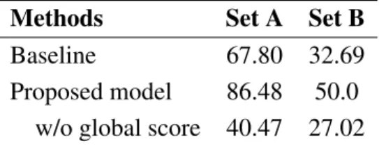
Methods Set A Set B

Baseline 67.80 32.69

Proposed model 86.48 50.0 w/o global score 40.47 27.02

Table 2: Accuracies on subsets of training (Set A) and validation (Set B) data.

instances in the validation set (Set B). We compare our baseline re-implementation with the proposed model on these sets. We also investigated the proposed model without global score.

The results are shown in Table 2. As can be seen, the accuracies improvement obtained with Sets A and B between baseline and the proposed method (about 19%) is greater than that obtained with the full validation set shown in Table 1 (about 4%). The decrease in accuracies between the proposed model with and without global score is also greater than that obtained with the full validation set. Furthermore, with Set B the baseline (32.69%) performs worse than its average (40.10%) on the full validation set, whereas the proposed model performs better (50.0% compared to 44.01%). Therefore, the results strongly indicate that the proposed model is better than the baseline at processing relationships between objects, which is largely due to the global score.

5.4.2 Instance Analysis

Figure 9 shows examples where the proposed model improves the baseline. As can be seen, the proposed method can select the correct object by matching the NP wooden chair to the green box and the NP lady to the red box (Figure 9, first row). On the other hand, the baseline model failed to select the correct object. In the second row of Figure 9, the proposed model correctly matched the NP a giraffe to the green bounding box and the NP a zebra to the red bounding box, whereas the baseline failed to capture the relationship and selected the wrong object, which is a zebra.

However, the proposed model also introduced some new errors. For example, in Figure 10 the Stanford CoreNLP incorrectly parsed the noun “woman” as a verb. As a result, only the NP ”cake” was extracted from the referring expression and the incorrect object was identified.

Another error is shown in Figure 11. In which, both the baseline and proposed models

A giraffe, standing to the right of a zebra.

A giraffe, standing to the right of a zebra.

A giraffe, standing to the right of a zebra.

Wooden chair to left of lady

Wooden chair to left of lady

Wooden chair to left of lady

Input Baseline Proposed Model

Figure 9: Examples where the proposed model improves the baseline.

Woman in a cream colored wedding dress cutting cake Woman in a cream colored

wedding dress cutting cake

Input Proposed Model

Figure 10: An error made by the proposed model.

failed to match the NP “a human hand” to the correct object in the image. Instead,

they matched the NP to some completely unrelated object (a pillow and a hamburger,

respectively). In our analysis, we found a significant portion of this type of errors, which

led us to reconsider the efficiency of the visual features being used. To this point, we

have used features extracted from the VGG model [18], which is considered to contain

abundant information about an object. However, as shown in Figure 11, it seems that

the visual features sometimes event fail to restore fundamental information such as

object category.

a human hand a human hand a human hand

Input Baseline Proposed Model

Figure 11: An error made by both the baseline and proposed models.

Baseline Proposed Model CNN vector(vgg) 40.10 44.01

Category label 57.69 61.77

Table 3: Accuracies with different visual representations on the validation set.

5.5 CNN Vector or Category Label as Visual Features?

In comparison to the visual features extracted from VGG, we experimented with the object category labels available in the Google Refexp dataset. These labels are automatically annotated by a classifier trained on the MSCOCO dataset [1]. They categorize objects into 80 classes, so we used a one-hot vector of dimension 80 to represent the label, and replaced the VGG vector with this one-hot vector as the visual features in our experiments.

The results are shown in Table 3. As can be seen, significant improvement was obtained by adopting the category information for both the baseline and proposed models. This indicates that (automatically recognized) category labels can represent the visual content of the object candidates more effectively. This may be due to the fact that the pretrained CNN model does not completely match the domain of objects in the Google Refexp dataset.

An example is shown in Figure 12. Here, the second column shows the output of

the proposed model using the VGG vector for the visual representation and the third

column shows the output using the one-hot category vector. As can be seen, with the

VGG vector, the NP “a man and a motorcycle” were matched to incorrect objects. In

contrast, with the one-hot category vector, the two NPs in the referring expression were

both matched to the correct objects.

a man on a motorcycle

a man on a motorcycle

a man on a motorcycle

Input CNN feature Category label

Figure 12: An example showing that the one-hot category vector is more helpful than the VGG vector.

To confirm the assumption that the visual feature extracted from the CNN rarely contains category information, we attempted to train a classifier for the 80 category labels from VGG vector extracted from object image. There are a total of 210775 objects in the Google Refexp dataset, and we randomly chose 200775 instances as training set and the remaining 10000 instances as test set. A two-layer fully connected neural network was adopted as the classifier. The results are 38.4% on the training set and 33.4% on the test set; quite low regarding the current literature of object category recognition.

5.6 Faster RCNN Vector as Visual Features

From section 5.5 we know that the visual feature extracted from the CNN rarely contains category information, we assume the reason is that the CNN vectors are extracted from VGG model which is trained on ImageNet dataset with classification loss function.

So we compare the CNN feature extracted from faster rcnn [24] model trained on MSCOCO dataset [2], the same dataset used in this thesis. The faster rcnn is designed for object detection and we use the output from RoI pooling layer. The results is shown in Table 4

Proposed Model

CNN vector(vgg) 44.01

CNN vectror(faster rcnn) 56.20

Table 4: Accuracies with different visual representations on the validation set.

5.7 Comparison with Related Work

In this section, we compare the proposed model with several previous works. First, we note that there are two different settings for evaluation; this is because most works on REC have used a large number of automatically detected objects to augment training, which is also the case in our study. We have used the automatic object detection results coming together with the Google Refexp dataset. The question is whether to include the automatically detected objects in test.

To this point, we have shown evaluation results with automatically detected objects included. This is because the proposed model heavily relies on recognizing relations with other objects, and this is the “multibox” setting in [1]. However, the more popular setting is to exclude automatically detected objects, and only test on the “ground truth” bounding boxes. Thus, we adopt the “ground truth” setting in this section for comparison.

To achieve this, we still use automatically detected objects during test, but only consider those bipartite graphs which align the head NP to a ground truth bounding box. Thus, the final output is always a ground truth object (though the model may additionally recognize its relationships with automatically detected objects).

The experimental results are shown in Table 5. Though the performance is a bit low when we use CNN vectors as visual features, we have achieved results comparable to the state-of-the-art by using category labels.

Accuracy CNN vector 50.3 Category label 64.0

[5] 64.0

[4] 68.4

[6] 69.3

Table 5: Accuracies evaluated on ground truth bounding boxes in the validation set.

6 Conclusion and Future Work

In this thesis, we have proposed a model for REC which considers relationships between

entities in a referring expression and align them to spatial relations between objects in

an image explicitly. The proposed model outperforms a baseline and we have shown

that modeling relationships is crucial for the performance gain. Furthermore, the

discovery that replacing a CNN feature vector with a one-hot category vector improves

performance is quite surprising. It raises concerns about the generalization ability of

deep neural representations – sometimes, human designed category labels can be more

generalizable.

Acknowledgements

I would like to express my gratitude to Professor Kentaro Inui, Associate Professor Naoaki Okazaki and Assistant Professor Ran, Tian for their supervision.

I would like to thank Dr. Ran, Tian for the discussion of the idea and implementation details of this thesis. Without his help it could be more difficult to finish the research of this thesis.

I would also express my gratitude to Assistant Professor Yuichiro, Matsubayashi for his kind discussion with me about the algorithm of my thesis.

I would like to express my gratitude to Professor Kentaro Inui, Associate Professor Naoaki Okazaki, Professor Yoshifumi Kitamura, Professor Takayuki Okatani for their supervision and guidance as the thesis committee of my master thesis.

Finally I would like to thank members in Inui-Okazaki Lab.

References

[1] Junhua Mao, Huang Jonathan, Alexander Toshev, Oana Camburu, Alan Yuille, and Kevin Murphy. Generation and comprehension of unambiguous object de- scriptions. arXiv preprint arXiv:1511.02283, 2015.

[2] Tsung-Yi Lin, Michael Maire, Serge J. Belongie, Lubomir D. Bourdev, Ross B. Gir- shick, James Hays, Pietro Perona, Deva Ramanan, Piotr Doll´ar, and C. Lawrence Zitnick. Microsoft COCO: common objects in context. CoRR, abs/1405.0312, 2014.

[3] Emiel Krahmer and Kees van Deemter. Computational generation of referring expressions: A survey. Comput. Linguist., 2012.

[4] Varun K. Nagaraja, Vlad I. Morariu, and Larry S. Davis. Modeling context between objects for referring expression understanding. CoRR, abs/1608.00525, 2016.

[5] Licheng Yu, Patrick Poirson, Shan Yang, Alexander C. Berg, and Tamara L. Berg.

Modeling context in referring expressions. CoRR, abs/1608.00272, 2016.

[6] Ronghang Hu, Marcus Rohrbach, Jacob Andreas, Trevor Darrell, and Kate Saenko.

Modeling relationships in referential expressions with compositional modular networks. CVPR2017, abs/1611.09978, 2016.

[7] Andrej Karpathy, Armand Joulin, and Fei-Fei Li. Deep fragment embeddings for bidirectional image sentence mapping. NIPS2014, abs/1406.5679, 2014.

[8] Andrej Karpathy and Fei-Fei Li. Deep visual-semantic alignments for generating image descriptions. CVPR2015, abs/1412.2306, 2015.

[9] Anna Rohrbach, Marcus Rohrbach, Ronghang Hu, Trevor Darrell, and Bernt Schiele. Grounding of textual phrases in images by reconstruction. CoRR, abs/1511.03745, 2015.

[10] Lu Cewu, Krishna Ranjay, Bernstein Michael, and Fei-Fei Li. Visual relationship

detection with language priors. 2016.

[11] M. Muraoka, S. Maharjan, M. Saito, K. Yamaguchi, N. Okazaki, T. Okatani, and K. Inui. Recognizing open-vocabulary relations between objects in images. 2016.

[12] Ilya Sutskever, Oriol Vinyals, and Quoc V. Le. Sequence to sequence learning with neural networks. CoRR, abs/1409.3215, 2014.

[13] Yonghui Wu, Mike Schuster, Zhifeng Chen, Quoc V. Le, Mohammad Norouzi, Wolfgang Macherey, Maxim Krikun, Yuan Cao, Qin Gao, Klaus Macherey, Jeff Klingner, Apurva Shah, Melvin Johnson, Xiaobing Liu, Lukasz Kaiser, Stephan Gouws, Yoshikiyo Kato, Taku Kudo, Hideto Kazawa, Keith Stevens, George Kurian, Nishant Patil, Wei Wang, Cliff Young, Jason Smith, Jason Riesa, Alex Rud- nick, Oriol Vinyals, Greg Corrado, Macduff Hughes, and Jeffrey Dean. Google’s neural machine translation system: Bridging the gap between human and machine translation. CoRR, abs/1609.08144, 2016.

[14] Kelvin Xu, Jimmy Ba, Ryan Kiros, Kyunghyun Cho, Aaron C. Courville, Ruslan Salakhutdinov, Richard S. Zemel, and Yoshua Bengio. Show, attend and tell:

Neural image caption generation with visual attention. CoRR, abs/1502.03044, 2015.

[15] Kaiming He, Xiangyu Zhang, Shaoqing Ren, and Jian Sun. Deep residual learning for image recognition. CoRR, abs/1512.03385, 2015.

[16] Olga Russakovsky, Jia Deng, Hao Su, Jonathan Krause, Sanjeev Satheesh, Sean Ma, Zhiheng Huang, Andrej Karpathy, Aditya Khosla, Michael S. Bernstein, Alexander C. Berg, and Fei-Fei Li. Imagenet large scale visual recognition challenge. CoRR, abs/1409.0575, 2014.

[17] Alex Krizhevsky, Ilya Sutskever, and Geoffrey E Hinton. Imagenet classification with deep convolutional neural networks. In F. Pereira, C. J. C. Burges, L. Bottou, and K. Q. Weinberger, editors, Advances in Neural Information Processing Systems 25, pages 1097–1105. Curran Associates, Inc., 2012.

[18] Karen Simonyan and Andrew Zisserman. Very deep convolutional networks for large-scale image recognition. CoRR, abs/1409.1556, 2014.

[19] Tomas Mikolov, Kai Chen, Greg Corrado, and Jeffrey Dean. Efficient estimation

of word representations in vector space. CoRR, abs/1301.3781, 2013.

[20] Jimmy Ba, Volodymyr Mnih, and Koray Kavukcuoglu. Multiple object recognition with visual attention. CoRR, abs/1412.7755, 2014.

[21] Christopher D. Manning, Mihai Surdeanu, John Bauer, Jenny Finkel, Steven J.

Bethard, and David McClosky. The Stanford CoreNLP natural language pro- cessing toolkit. In Association for Computational Linguistics (ACL) System Demonstrations, pages 55–60, 2014.

[22] S. Tokui, K. Oono, S. Hido, and J. Clayton. Chainer: a next-generation open source framework for deep learning. NIPS Workshop on Machine Learning Systems(LearningSys), 2015.

[23] Diederik P. Kingma and Jimmy Ba. Adam: A method for stochastic optimization.

CoRR, abs/1412.6980, 2014.

[24] Ross Girshick Jian Sun Shaoqing Ren, Kaiming He. Faster R-CNN: To-

wards real-time object detection with region proposal networks. arXiv preprint

arXiv:1506.01497, 2015.

List of Publications

Other Publications

Ran Wensheng, Tian Ran, Okazaki Naoaki, Inui Kentaro. Modeling Relationships

between Objects for Referring Expression Comprehension. Special Interest Group of

Natural Language Processing (IPSJ-SIGNL) Information Processing Society of Japan,

SIGNL 226, July.2017