HUSCAP Journals

Instructions for use

T itle E xtending the Picard-F uchs system of local mirror symmetry

A uthor(s ) F orbes,B rian; J inzenji,Masao

C itation Hokkaido University Preprint S eries in Mathematics, 712: 1-47

Is s ue D ate 2005

D O I 10.14943/83863

D oc UR L http://hdl.handle.net/2115/69517

T ype bulletin (article)

Extending the Picard-Fuchs system of local

mirror symmetry

Brian Forbes, Masao Jinzenji

Division of Mathematics, Graduate School of Science

Hokkaido University

Kita-ku, Sapporo, 060-0810, Japan

[email protected]

[email protected]

March, 2005

Abstract

We propose an extended set of differential operators for local mirror symmetry. If X

is Calabi-Yau such that dimH4(X,Z) = 0, then we show that our operators fully describe

mirror symmetry. In the process, a conjecture for intersection theory for suchXis uncovered. We also find new operators on several examples of typeX=KS through similar techniques.

In addition, open string PF systems are considered.

1

Introduction.

For some time now, mirror symmetry has been successfully used to make enumerative predictions on certain Calabi-Yau manifolds. While mirror symmetry for compact Calabi-Yau’s has been extensively studied, local mirror symmetry is relatively new, and a complete formulation does not yet exist.

The first unified treatment of local mirror symmetry was written down in [5], in the case that the space looks like X = KS, where S is a Fano surface and KS is its canonical bundle. Very

recently [17], the work of [5] was formulated more mathematically. With the ideas of [17], we are able to determine all information relevant for mirror symmetry directly from the Picard-Fuchs equations of the mirror. These techniques are limited to the case that X satisfiesb2(X) =b4(X).

mirror symmetry constructions of [5], our methods still complete missing data; however, a general formulation here is lacking.

The key point in the construction of the extended Picard-Fuchs system is the determination of triple intersection numbers of K¨ahler classes for open Calabi-Yau manifolds. Up to now, a natural definition of triple intersection numbers of K¨ahler classes on open Calabi-Yau manifolds is not known, but in this paper, we search for triple intersection numbers that are “natural” from the point of view of mirror symmetry in the sense of the following conjecture:

Conjecture 1 Consider the A-model on a Calabi-Yau threefold X. Let ui be the logarithm of

the B-model complex deformation parameter zi obtained from the toric construction of the mirror

Calabi-Yau manifold Xˆ. Then the B-model Yukawa coupling Cuiujuk of Xˆ obtained from the

A-model Yukawa coupling of X is a rational function in zi = exp(ui). Moreover, its denominator

includes the divisor of the defining equation of the discriminant locus of Xˆ.

Since the triple intersection number is just the constant term of the B-model Yukawa coupling

Cui_uj_uk, the above conjecture imposes constraints on these triple intersection numbers. In this paper, we regard these triple intersection numbers as intersection numbers of some minimal com-pactification X of X. With these intersection numbers in hand, we can construct a quantum cohomology ring of X and an associated Gauss-Manin system. In the examples treated in this paper, this quantum cohomology ring satisfies Poincare duality as a compact 3-fold, even ifX is an open Calabi-Yau 3-fold. With this Gauss-Manin system, we can write down differential equations for ψ0(ti), the function associated to the identity element of the quantum cohomology ring. Then

we can rewrite these differential equations by using the mirror map ti =ti(z∗). Our assertion in

this paper is that the differential equations so obtained are the extension of the Picard-Fuchs op-erators obtained from the standard toric construction of ˆX. Moreover, the extended Picard-Fuchs system has all the properties that the Picard-Fuchs system associated to a compact Calabi-Yau 3-fold should have: a unique triple log solution, Yukawa couplings, etc.

One problem in the construction is that in some cases, the constraints obtained from the above conjecture are not strong enough to determine all the triple intersection numbers. In other words, we have some real moduli parameters in the triple intersection numbers. Yet, we can still construct the extended Picard-Fuchs system for each value of the moduli parameters, and these systems have all the properties desired for a Picard-Fuchs system associated to a compact Calabi-Yau 3-fold. In the case that b4(X) =b6(X) = 0, we find unique triple intersection numbers

compatible with the above conjecture by considering the change of the prepotential under flops. Hence, our construction of an extended Picard-Fuchs system has no ambiguity in this situation.

Here is the organization of the paper. Section 2 spells out the generalities of the Gauss-Manin system and intersection theory for open Calabi-Yau manifolds. In Section 3, we thoroughly consider O(−1)⊕ O(−1)→P1, giving a PF operator for mirror symmetry and a geometric view of the meaning of the operator. Section 4 is the generalization, which spells out a conjecture on how to deal with all X such that dimH4(X,Z) = 0. This is subsequently applied to several cases

Acknowledgements. We first would like to thank Fumitaka Yanagisawa for giving us a lot of help on computer programming. We would also like to thank Professor Martin Guest for discussions on quantum cohomology. B.F. would like to thank Professor Shinobu Hosono for helpful conversations, and Martijn van Manen for computer assistance. The research of B.F. was funded by COE grant of Hokkaido University. The research of M.J. is partially supported by JSPS grant No. 16740216.

2

The Main Strategy: Overview of the Gauss-Manin

Sys-tem.

Suppose that we have obtained “natural” classical triple intersection numbers

Xka∧kb∧kc for an

open Calabi-Yau 3-foldX under the assumption of Conjecture 1, and that we know the instanton part of the prepotential for X. Let us denote this instanton part by Finst_(t

∗) , where ta is the

K¨ahler deformation parameter associated to the K¨ahler form ka (a = 1,· · · , h1,1(X)). With this

data, we can construct an A-model Yukawa coupling for X:

Yabc(t∗) =

X

ka∧kb ∧kc+

∂3_Finst_(t

∗)

∂ta∂tb∂tc

. (2.1)

Using the classical intersection numbers

Xka ∧kb ∧ kc, we can construct a basis mα (α =

1,· · · , h1,1_{(X)) ofH}4_{(X,Z) that has the following property:}

ηaα:=

X

ka∧mα =δaα. (2.2)

With this setup, we obtain a (virtually compact) quantum cohomology ring ofX,

ka◦1 = ka,

ka◦kb =

c,γ

Yabc(t∗)ηcγmγ =

γ

Yabγ(t∗)mγ,

ka◦mα = Yaα0v =δaαv,

ka◦v = 0, (2.3)

where we used standard property of quantum cohomology ring:

Yaα0 =ηaα. (2.4)

Here v is the volume form of X and we use the subscript 0 to denote the identity 1 of H∗_(X,Z).

Then we consider the associated Gauss-Manin system:

∂aψ0 = ψa,

∂aψb =

c,γ

Yabc(t∗)ηcγψγ =

γ

Yabγ(t∗)ψγ,

∂aψα = Yaα0ψv =δaαψv,

Next, we consider the inverse matrix (Y−1

a (t∗))bc of (Ya(t∗))bc:=Yabc(t∗). From (2.5), we obtain,

ψα =

b

(Y_a−1(t∗))αb∂a∂bψ0. (2.6)

Since, ψα is unique for each α, we have to impose integrability conditions:

c

(Y_a−1(t∗))αc∂a∂cψ0 =

c

(Y_b−1(t∗))αc∂b∂cψ0 (a=b) (2.7)

for any a, b _{∈ {}1,2,_{· · ·} , h1,1_{(X)}. We have another integrability condition from the third line of}

(2.5):

∂a c

(Y−1

a (t∗))ac∂a∂cψ0

=∂b c

(Y−1

b (t∗))bc∂b∂cψ0

, (a=b)

∂b c

(Y_a−1(t∗))ac∂a∂cψ0

= 0, (a=b). (2.8)

for any a, b ∈ {1,2,· · · , h1,1_{(X)}. Finally, we can derive differential equations from the fourth}

line of (2.5):

∂_a2

c

(Y_a−1(t∗))ac∂a∂cψ0

= 0. (2.9)

Our strategy in this paper is to translate the equations (2.7), (2.8) and (2.9) in terms of the mirror map

ta =ta(z∗) (2.10)

into the differential equations of the complex deformation parameters za of the mirror manifold

ˆ

X. Of course, in the one parameter case, the equations (2.7) and (2.8) become trivial, and the only nontrivial equation is

∂_t2

1

Yttt

∂_t2ψ0(t) = 0, (2.11)

which is well-known from the literature.

In the following, we will explicitly compute (2.7), (2.8) and (2.9) in many examples, and we find that these equations are highly degenerate. Therefore, in this paper, we will choose the minimal independent set of equations for an extended Picard-Fuchs system.

By construction, the Picard-Fuchs system so obtained has a solution space given by

1, t1, . . . , th1,1_(X),

∂_F ∂t1

, . . . , ∂F ∂th1,1_(X)

,2_{F −}

h1,1

(X)

a=1

ta

∂_F ∂ta

. (2.12)

3

Mirror symmetry for local

P

.

3.1

A Picard-Fuchs operator for local

P

.

Before diving into the details of Gauss-Manin systems and the like, we will first take a simple-minded look at a familiar example, namely _O(₋1)_{⊕ O}(₋1)_→P1. We will see that in trying to apply the techniques of local mirror symmetry to this basic case, we are inevitably led to introduce the generalized intersection theory explained in the introduction. In fact, this is the example that originally motivated the investigations of this paper.

Recall the symplectic quotient definition ofO(−1)⊕ O(−1)→P1:

X ={(w1, . . . , w4)∈C4−Z :|w1|2+|w2|2− |w3|2− |w4|2 =r}/S1. (3.13)

Above, Z ={w1 =w2 = 0},r∈ R+ and

S1 _{: (w}

1, . . . , w4)→(eiθw1, eiθw2, e−iθw3, e−iθw4).

We can naively employ the methods of [17] to produce a Picard-Fuchs operator associated to the mirror Calabi-Yau ˆX of X. The family ˆX is described as [15]

ˆ

Xz ={(u, v, y1, y2)∈C2×(C∗)2 :uv+ 1 +y1+y2+zy1y−21 = 0}. (3.14)

Then [17] provides a recipe for dealing with non-compact period integrals for such an ˆX. They are defined by

ΠΓ(z) =

Γ

dudvdy1dy2/(y1y2)

uv+ 1 +y1+y2+zy1y2−1

for Γ ∈ H4(C2 ×(C∗)2 −X,ˆ Z). As usual, we utilize the GKZ formalism in order to exhibit an

differential operator which annihilates the ΠΓ. One finds

D= (1₋z)θ2, θ =z d

dz (3.15)

as the relevant PF operator.

This is a puzzling situation. Clearly, the solutions of _Df = 0 are given by _{1,logz_}. This is sensible, because noncompact PF systems always have a constant solution [5], and the mirror map is trivial in this case, leading to a logz solution. However, there is no double logarithmic solution, because _D is only of order 2. Hence, we have no function _F with which to count holomorphic curves on X! But, since X contains exactly 1 holomorphic curve, we know that the sought after function should be of the form

F(z) = K(logz)

3

6 +

n>0

zn

n3. (3.16)

Here K is a classical triple intersection number forP1 ֒→X.

At this point, we can gain a bit of insight from the compact case. Recall [6] that in the event of a compact Calabi-Yau X with one K¨ahler parameter, there is always a flat coordinate t in which the Picard-Fuchs operator for the mirror family is given as

Dcompact(t) =∂t2 1

Y ∂

2

t, (3.17)

which is the same as the formula (2.11). This is reminiscent of our situation (3.15), upon making the identification t = logz.

If one surrendered to the impulse of emulating the above compact expression, one would be compelled to work with the following modified differential operator:

D −→ D′ =θ2_D.

Rewrite this as

θ2(1−z)θ2 =θ2 1

1₋z

−1

θ2.

By comparison with (3.17), it is natural to identify the Yukawa couplingY of_O(₋1)_⊕O(₋1)_→P1

as

Y = 1

1−z. (3.18)

And indeed, the condition that Y =θ3_{F, which follows from the form of D}′_{, yields the expected}

function F (3.16). Then the resultant period vector is

Π′ = (1,logz, θ_F,2_{F −}(logz)θ_F),

which is the period vector encountered when dealing with compact Calabi-Yaus. Hence, we have found a ‘cure’ for mirror symmetry on X = _O(₋1) _{⊕ O}(₋1) _→ P1; the new operator θ2_D

reproduces all relevant data to describe mirror symmetry for X.

We can also view thisθ2_{D from the vantage of the Frobenius method. The geometry ofX is}

determined by the set of vertices _{ν0, . . . , ν3}={(0,0),(1,0),(0,1),(1,1)}, together with a choice

of triangulation of the resulting toric graph. These give rise to the lattice vectorl = (1,1,₋1,₋1), and identify z as the correct variable on the complex moduli space of ˆX.

Then the solutions of our extended PF operator θ2_{D can be generated, via the Frobenius}

method, from the function ω0(z, ρ) =_n≥0c(n, ρ)zn+ρ, with

c(n, ρ) = (Γ(1 +n+ρ)2Γ(1−n−ρ)2)−1.

It is a simple matter to verify that

Π′ = (ω0(z,0), ∂ρω0(z, ρ)|ρ=0, ∂ρ2ω0(z, ρ)|ρ=0, ∂ρ3ω0(z, ρ)|ρ=0).

Clearly this had to be the case, since the extension of the original _D on the left by each factor of

θ adds one more Frobenius-generated solution.

a unique choice which is compatible with the solutions ofθ2_{D, which turns out to beK = 1. This}

is the same as was used in the physical considerations of [27]. Later, we will see that the choice more natural for generalization is K = 1/2.

Next, we will take up the question of the geometric meaning of the solutions of this new operator.

3.2

PF extensions and Riemann surfaces.

In physics literature [2] [17], a frequently used technique of local mirror symmetry is to consider periods on a Riemann surface Σ֒_→Xˆ, rather than periods of the full mirror geometry ˆX. In this section, we will review evidence in favor of this approach.

Looking back at the mirror geometry (3.14), this can be rewritten as

ˆ

Xz ={uv+ 1 +y1 +y2+zy1y2−1 =uv+f(z, y1, y2) = 0},

which is a hypersurface in C2_×(C∗)2_{. Notice that there is an imbedded Riemann surface in this}

space, defined as

Σz ={(y1, y2)∈(C∗)2 :f(z, y1, y2) = 0}. (3.19)

In fact, this statement applies not only to the localP1 case, but to all toric local mirror symmetry constructions [2]. The only difference is that there may be more complex moduli involved; in such cases, we can simply set z = (z1, . . . , zn), where now each zi is a complex structure modulus.

Now take (a0, . . . , a3) as homogeneous coordinates on the moduli spaces of ˆX and Σ, i.e.

ˆ

Xa={uv+a0+a1y1+a2y2+a3zy1y2−1 =uv+f(a, y1, y2) = 0}.

Recall that the GKZ operators are differential operators _{Li} in the variablesa, such that

Li

Γ

dudvdy1dy2/(y1y2)

uv+f(a, y1, y2)

= 0, _∀i.

We can recover the PF operators from the GKZ operators via a canonical reduction on the homogeneous moduli space.

With these things in mind, we note the general

Proposition 1 The GKZ operators associated to the geometryXˆ are the same as those associated to Σ.

Proof. Notice that Σ is a complex dimension 1 noncompact Calabi-Yau manifold. In particular, it makes sense to define the period integrals of Σ as

ΠΣ_γ(a) =

γ

dy1dy2/(y1y2)

f(a, y1, y2)

with γ _∈H2((C∗)2−Σ,Z). Let L be a GKZ operator on the moduli space of Σa, so that

Recall that the period integrals of ˆXa are given as

ΠX_Γˆ(a) =

Γ

dudvdy1dy2/(y1y2)

uv+f(a, y1, y2)

(3.20)

for Γ_∈H4(C2×(C∗)2−X,ˆ Z). Then it is clear that we must also have

LΠX_Γˆ(a) = 0,

because the additive factor of uv in the period integrals of ˆX is independent of a. Clearly the converse of this statement is also true, so the proposition follows.

Note that, as pointed out in [17], there us a subtlety in terms of the scaling properties of the period integrals on ˆXa and Σa. Further, this scaling difference implies that the PF operators we

derive from the above_L will be different on Σz and ˆXz. In the following, we will ignore this point,

and carry on as though the period integrals on Σz actually reproduce the same PF operators.

As the geometry of Σ is far simpler than that of ˆX, this proposition will greatly aid the search for a geometric interpretation of the formal procedure _{D →}θ2_{D on Picard-Fuchs operators. We}

will explore this in the next section.

3.3

Geometric interpretation through the Riemann surface.

First, we will give a brief description of what “adding extra period integrals” means (which we are doing, by raising the power of the PF operator) in the context of the space ˆX. This follows the lead of e.g. [15],[4].

Recall that mirror symmetry between the spacesX and ˆX means, in particular, that

dimH1,1(X) = dimH2,1( ˆX).

Hence, for every 2 cycle of X, we can expect a mirror 3 cycle of ˆX. Let dimH3( ˆX,Z) = n,

and take Γi,Γj ∈ H3( ˆX,Z) with Poincar´e duals αi, αj ∈ H3( ˆX,Z). Then there is a symplectic

structure on H3( ˆX,Z), defined by the intersection pairing

(Γi,Γj) =

ˆ

X

αi∧αj.

In the compact case, we can find a basis _{Φ1, . . . ,Φn/2,Ψ1, . . . ,Ψn/2}for H3( ˆX,Z) satisfying

(Φi,Φj) = (Ψi,Ψj) = 0 , (Φi,Ψj) =δij.

However, there is no such nice construction for the noncompact case. In fact, we can explicitly exhibit this failure in the example we are considering, _O(₋1)_{⊕ O}(₋1)_→ P1. First, rewrite the equation for the mirror ˆX:

ˆ

where we have taken ˜yi =yi−1 and ˜u=u/y1y2. Set z = 1−a, where a∈R+. Then

ˆ

Xz ={uv˜ + 1 + ˜y1+ ˜y2+ ˜y1y˜2 =a},

and we can identify a 3 cycle

Γ1 = ˆXz∩ {u˜= ¯v,y˜2 = ¯˜y1}={vv¯+ (1 + ˜y1)(1 + ˜y1) =a}.

It is easy to verify that this cycle has no symplectic dual in H3( ˆX,Z).

Of course, there is a noncompact symplectic dual for Γ1. Let p∈Γ1, and take ˜Γ1 = (NΓ1/Xˆ)p. Then ˜Γ1 intersects Γ1 in a point, and could be thought of as a dual; however, integrals over ˜Γ1

may not be well defined. Instead take

˜

Γλ₁ =_{v _∈(N_Γ1/Xˆ)p :|v| ≤λ}, λ∈R+.

Set

Ω_Xˆ = Res{uv+f(z,y1,y2)=0}

dudvdy

1dy2/(y1y2)

uv+f(z, y1, y2)

.

Then the proposal of [15] is that we should also consider integrals of the form

˜ Γλ

1 Ω_Xˆ

as periods of the noncompact geometry ˆX. Mathematically, this means that the definition of noncompact period integrals of ˆX are to be taken as all

ΓΩXˆ for Γ ∈ H3( ˆX,Z)⊕(H3( ˆX,Z))c.

Here, the subscript c indicates compactly supported homology. In view of Proposition 1, one can make the following

Definition 1 Let Xˆ be the noncompact Calabi-Yau hypersurface

ˆ

X =_{(u, v, y1, y2)∈C2×(C∗)2 :uv+f(z, y1, y2) = 0}

and Σ the imbedded Riemann surface Σz = ˆX∩ {u =v = 0}. Then the period integrals of ˆX are

defined to be

Πγ(z) =

γ

Resf=0

dy₁dy₂/(y₁y₂)

f(z, y1, y2)

for γ _∈H1(Σ,Z)⊕(H1(Σ,Z))c.

3.4

Period integrals for local

P

.

Before describing the cycles of Σ and computing their associated integrals, we will need to make use of the following proposition. This will give a (1,0) form α ∈ H1(log(Σ),Z), which can be

integrated over lines in Σ. Note that, as was the case of the previous proposition, the validity is for all Riemann surfaces appearing as mirrors of the toric local mirror symmetry construction.

Some of the arguments below can be found in [22].

Proposition 2 Let Σ be as above, and choose γ _∈H1(Σ,Z)⊕(H1(Σ,Z))c. Then

γ

Resf=0

dy

1dy2/(y1y2)

f(z, y1, y2)

=−

γ

logy2

dy1

y1

=−

γ

logy1

dy2

y2

.

Proof. LetT(γ) be a tubular neighborhood ofγ in Σ. One easily sees that the PF operators of

T(γ)

dy1dy2/(y1y2)

f(z, y1, y2)

and

T_(γ)

log(f)dy1dy2/(y1y2)

are in fact the same. Then, if we assume that Definition 1 gives an equivalence between PF solutions and period integrals, we have

γ

Resf=0

dy₁dy₂/(y₁y₂)

f(z, y1, y2)

=

γ

Resf=0

log(f)dy1dy2/(y1y2) =

−

γ

Resf=0

d(log(f)) logy2

dy1

y1

=₋

γ

Resf=0

df

f logy2 dy1 y1 = − γ

logy2

dy1

y1

.

From the first to the second line, we have integrated by parts, and then the residue aroundf = 0 was taken from the second to third line.

This argument applies equally well upon exchanging y1 and y2.

With this proposition in hand, we can take up the task of working out period integrals on local

P1_{. Recall that the original, unmodified PF operator for this space was found to be}

D = (1₋z)θ2,

with solution set_{1,logz_}. We will at first content ourselves with finding cyclesγ0, γ1 ∈H1(Σ,Z)

whose period integrals reproduce these solutions. To this end, note that the defining equation

Σ =_{(y1, y2)∈(C∗)2 : 1 +y1+y2+zy1y2−1 = 0} (3.21)

can be solved in 2 ways:

y1 = −

1₋y2

1 +zy₂−1, y

±

2 =

−1₋y1±

(1 +y1)2−4zy1

Now, sincey1andy2areC∗ variables, we can define three homology elements from these equations:

γ0 =

(y1, y2)∈(C∗)2 :y1 = −

1−y2

1 +zy−₂1 , |y2|=ǫ

,

τ± =

(y1, y2)∈(C∗)2 :y2±=

−1−y1±

(1 +y1)2−4zy1

2 , |y1|=ǫ

.

Then, two of these must be responsible for the solution set {1,logz}. To motivate the correct choice of cycles, let us first look closely at the mirror construction that originally provided equation (3.21).

Starting with the description O(−1)⊕ O(−1)→P1 ₌

{(w1, . . . , w4)∈C4−Z :|w1|2+|w2|2− |w3|2− |w4|2 =r}/S1,

from [2], the mirror geometry can be characterized as

{uv+x1+· · ·+x4 = 0 :x1x2x−31x−41 =z, xi = 1 for some i}.

Here u, v _∈ C and xi ∈ C∗. Also, the xi obey |xi| = exp(−|wi|2), and |z| = e−r. To arrive at

the form (3.21), we set x3 = 1 and solved for x1 in the constraint x1x2x−31x−41 = z. Finally, the

identification y1 =x4, y2 =x2 was made.

The equation for local P1 indicates that [w1, w2] can be taken as homogeneous coordinates

on the P1. In the locus where w3 = w4 = 0, we thus have a bound 0 ≤ |w2|2 ≤ r. Then

|y2|= exp(−|w2|2) implies that 1≥ |y2| ≥e−r =|z|; taking these considerations together, we may

accurately label the following figure:

γ0

γ1

τ−

τ+

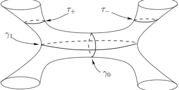
Figure 1: 1-cycles on Σ. _{γ0, τ+, τ−} is a basis for H1(Σ,Z).

Proposition 3 Let γ0, τ± be as described above, and set

γ1 = [τ+] + [τ−]

with the sum taken in H1(Σ,Z). Then

γ0 logy1

dy2

y2

= 1,

γ1 logy2

dy1

y1

= logz

Proof. The first integral is trivial:

γ0 logy1

dy2

y2

=

|y2|=ǫ

log−1−y2 1 +zy₂−1

dy2

y2

=

|y2|=ǫ

iπ+ log 1 +y2 1 +zy2−1

dy₂

y2

and this is a constant. Of course, the branch cut of log must be taken to lie off the negative real axis.

For the second,

γ1 logy2

dy1

y1

=

τ+

logy₂+ dy1 y1

+

τ−

logy−₂ dy1 y1

=

|y1|=ǫ

log(y+₂y₂−)dy1

y1

=

|y1|=ǫ

log(zy1)

dy1

y1

=const+ 2πilogz.

Next, the existence of a new period integral, based on Definition 1, will be demonstrated.

3.5

A period integral from

(

H

(Σ

,

Z

))

Since the constraint 1 _{≥ |}y2| ≥ |z| only applies in regions with z3 =z4 = 0, outside of this locus,

it is sensible to define a path on Σ as follows. Let λ < |z| be real, and take a smooth increasing function σ : [0,1] :_→Σ such that σ(0) =λ, σ(1) =z. Then

γ2(λ) =

(y1, y2)∈(C∗)2 :y1 = −

1−y2

1 +zy₂−1, y2 =σ[0,1], y1 = 1

defines an element of (H1(Σ,Z))c.

Proposition 4 Let Σ, γ2 be defined as above. Then

θF =

γ2 logy1

dy2

y2

,

where θ=z d

dz and θF is the double logarithmic solution of the extended PF operator

D′ _=θ2_(1−z)θ2

associated to the mirror of the local model _O(₋1)_{⊕ O}(₋1)_→P1.

Proof. The computation is straightforward:

γ2 logy1

dy2

y2

=

z

λ

log−1−y2 1 +zy−1 2

dy2

y2

z

λ

iπ+

n>0

(−y2)n

n −

n>0

(−zy₂−1)n

n

dy2

y2

=

const+ (λ−dependent) +

n_>0

(−z)n

n2 =

θF

(−z).

In order to achieve the result, we should have z rather than ₋z in the above. However, this is accounted for by the fact that arg(y2) is not determined in local mirror symmetry, and hence we

are free to use the variable y′

2 =eiπy2 in place ofy2.

Notice that, with this definition of period integrals, the logarithmic terms of θ_F are not uniquely determined, as they depend on λ. It is for this reason that λ dependent terms are disregarded in the calculation.

It may seem that the choice of γ2 is artificial, since we could have equally well chosen an

increasing function σ′ _{: [0,1]→Σ with σ}′_{(0) = 1, σ}′_{(1) = λ >1. However, it is easy to show that}

this is equivalent; if

γ₂′(λ) =(y1, y2)∈(C∗)2 :y1 = −

1−y2

1 +zy₂−1, y2 =σ

′_{[0,1], y}

1 = 1

,

then

lim

λ→∞

θ

γ′

2 logy1

dy2

y2

=

n>0

(₋z)n

n ,

so the two approaches are interchangeable.

3.6

Discussion.

So far, we have considered only one example: _O(₋1)_{⊕ O}(₋1)_→P1. However, we have learned a great deal already. Firstly, the PF system cannot always be relied on to provide all the information we need for local mirror symmetry. Yet, one might be tempted to hope that, in general, we can recover the missing data through a simple modification of the known PF systems. Let us consider our new operator θ2_{D from one final perspective.}

The incompleteness of the PF system onX=O(−1)⊕O(−1)→P1_{is supposed to emerge from}

the noncompactness of the space; that is, as a result of the facts thatb4 =b6 = 0, wherebi denotes

the ith Betti number. On a compact space, the PF system will have one regular solution, b2(resp.

b4) logarithmic (resp. double logarithmic) solutions, and one (= b6) triple logarithmic solution.

On X, our two usual PF solutions can be summarized by a cohomology-valued hypergeometric series [12][16][17]

ω(z, J) = ω0+ω1(z)J.

Here ω0 = 1, and ω1 = logz is the mirror map. Also, J is the cohomology element dual to

P1 ֒_→X. Solutions of the PF system _Df = 0 are recovered asωi(z) = d

i_ω(z,J)

dJi |J=0.

It is clear that by instead working with θ2_{Df = 0, we have a larger cohomology-valued series}

as a generating function of solutions:

From this perspective, the addition of θ2 _{on the left-hand side of the operator D is a sort of}

compactification of the model, in that it represents the addition of a 4-cycle and a 6-cycle forX. We will now generalize these ideas to situations with no 4-cycle, and an arbitrary number of K¨ahler classes.

4

Mirror Symmetry for Toric Trees.

In this section, we will show that ifXis a noncompact Calabi-Yau manifold such that dimH4(X,Z) =

0, then we may apply our methods to obtain a complete system of differential equations which fully determines the prepotential. The Yukawa couplings take on a central role in the following.

4.1

Ordinary Picard-Fuchs systems.

Our first interest will be to take a look at the PF systems one would arrive at through use of existing local mirror symmetry techniques. We wish to understand exactly how much information one might recover through these systems alone, in order to determine an appropriate ‘fix’.

Let us clarify what we are exploring here. Let {l1_{, . . . , l}n_{} ⊂ Z}m _{be a choice of basis for}

the secondary fan of a noncompact toric Calabi-Yau threefold X satisfying dimH4(X,Z) = 0.

Consider the generating function

ω(z, ρ) =

n>0

c(n, ρ)zn+ρ (4.22)

where

c(n, ρ)−1 =

i

Γ

1 +

k

lk_i(nk+ρk)

. (4.23)

Here we are using the convention that lk _{= (l}k

1, . . . , lkm). Then we want to look at the functions

Πij =

∂ρi∂ρjω(z, ρ)

|ρ= 0. (4.24)

Our interest in this subsection, then, is to ascertain how much information we can find by looking at the Πij. In so doing, we will gain a better understanding of what to do in order to remedy

mirror symmetry in this situation.

Example 1 Consider the space

X1 ={−2|w1|2+|w2|2+|w3|2=Re(t), |w1|2− |w2|2+|w4|2− |w5|2 =Re(s)}/(S1)2

where (w1, . . . , w5)∈C5−({w2 =w3 = 0} ∪ {w1 =w4 = 0} ∪ {w4 =w5 = 0}). This contains two

curves Ct, Cs with respective normal bundles O ⊕ O(−2) and O(−1)⊕ O(−1) in X1. We have

that b2 = 2 andb4 = 0.

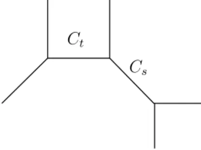
From the work [23], we can draw a planar trivalent graph for X1 corresponding to the torus

Cs

Ct

Figure 2: Toric diagram for X1.

we have the PF operators associated to X1:

D1 = θ1(θ1−θ2)−z1(2θ1 −θ2)(2θ1−θ2+ 1)

D2 = (2θ1−θ2)θ2−z2(θ1 −θ2)θ2

D3 = θ1θ2 −z1z2(2θ1−θ2)θ2. (4.25)

Let ω(z, ρ) be the generating function for solutions of this, with logarithmic solutions t, s.

Set Πij = ∂ρi∂ρjω|ρ=0. Then {D1,D2} also has a double logarithmic solution, given as the linear combination

W(z) = 1

2Π11+ Π12+ Π22.

We are interested in the relationship between this double logarithmic solution and the prepo-tential _F1 for X. From physics [9][18], the instanton part of the prepotential is

F1inst=

n>0

ens

n3 +

en(s+t)

n3 −

ent

n3. (4.26)

Naturally, this is the expression gotten after use of the inverse mirror map. Let us first take a look at the Πij’s, after the insertion of the mirror map:

Π11(s, t) = 0,

Π12(s, t) =

n>0

en(t+s)

n2 −

ens

n2 ,

Π22(s, t) = 2

n>0

ens

n2.

We have neglected the logarithmic terms of each function. Notice that there is no linear combi-nation of Πij’s that we can take to reproduce the term _n>0ent/n2.

From these expressions,

W(s, t) =

n>0

en(s+t)

n2 +

ens

n2 =

∂_Finst

1

∂s .

Example 2 Next, consider the space

X2 ={|w1|2+|w2|2− |w3|2− |w4|2 =Re(s1), −|w1|2− |w3|2+|w4|2+|w5|2 =Re(s2)}/(S1)2,

with (w1, . . . , w5) ∈ C5 −({w1 = w2 = 0} ∪ {w4 = w5 = 0} ∪ {w2 = w5 = 0}). We again have

b2 = 2, b4 = 0, and now NCi/X2 ∼=O(−1)⊕ O(−1) for each i. Notice that we can flop fromX2 to

X1: if l1 = (1,1,−1,−1,0) and l2 = (−1,0,−1,1,1), then the combinations l1+l2,−l2 give the

secondary fan for X1. The planar trivalent toric graph for X2 is given in figure 3. We have the

Cs1

Cs2

Figure 3: Toric diagram for X2.

PF system from the mirror manifold:

D1 = (θ1−θ2)θ1−z1(−θ1−θ2)(−θ1+θ2),

D2 = (θ2−θ1)θ2−z2(−θ2−θ1)(−θ2+θ1),

D3 = θ1θ2−z1z2(θ1+θ2+ 1)(θ1+θ2). (4.27)

Let si be the logarithmic solutions. Using the same conventions as example 1, we find

Π11(s1, s2) =

n>0

ens1

n2 −

ens2

n2 ,

Π12(s1, s2) = 0,

with Π22 =−Π11. Again, these expressions already include the mirror map.

Let’s take a look at the prepotential:

Finst

2 =

n≥0

ens1

n3 +

ens2

n3 −

en(s1+s2)

n3 .

Then we see that

Π11 =

∂_Finst

2

∂s1 −

∂_Finst

2

∂s2

.

Hence, we could recover a bit of information by using the basic extended system{θ1D1,D2}, which

Our work with example 1 suggests the reason for the problem with theCs1+s2 curve. To exhibit this, recall that the lattice vectors _{l1_{, l}2_{} for this geometry are}

l1

l2

=

1 1 ₋1 ₋1 0 0 ₋1 ₋1 1 1

Each vector represents a curve Csi in X2.Then Cs1+s2 is determined by the single vector

l1+l2 =

1 0 −2 0 1

.

This curve satisfies NCs1 +s2/X2 ∼= O ⊕ O(−2). Hence, we do not expect that we can retrieve its information from the PF system.

We have performed similar computations for 3 and 4 parameter cases, all of which support this general principle. This leads us to make the

Conjecture 2 LetX be a noncompact toric Calabi-Yau threefold withdimH4(X,Z) = 0, and say

{l1_{, . . . l}m_{} defineX via symplectic quotient. Letω =}

n>0c(n, ρ)zn+ρ be the generating function

for

Πinst_ij =

n

∂ρi∂ρjc(n, ρ)

|ρ=0zn (4.28)

with

c(n, ρ)−1 =

i

Γ

1 +

k

lk_i(nk+ρk)

. (4.29)

If _F is the prepotential, andsi =∂ρiω|ρ=0 for each i such that

li =

1 1 −1 −1 0 . . . 0

(up to a permutation of the columns of li_{), then there are rational numbers m}

ij ∈Q such that

i,j

mijΠinstij =

i

(₋1)i−1∂F

inst

∂si

.

Here, Finst _{is the instanton part of the prepotential. We use the notation Π}inst

ij to distinguish

these functions from the usual derivatives of ω (i.e. Πij =∂ρi∂ρjω|ρ=0).

This conjecture is equivalent to the statement that although we cannot detect curves with normal bundleO⊕O(−2) via the Πij, we can exhibit all curves with normal bundleO(−1)⊕O(−1)

using these functions.

4.2

Two building blocks of solutions.

Assume X is a noncompact Calabi-Yau threefold such that dimH4(X,Z) = 0, and that every two

cycle C ֒→X has normal bundleO ⊕ O(−2) or O(−1)⊕ O(−1). We will refer to these as t and

s curves, respectively, in the following.

Then, as any such space X is obtained by gluing s and t curves together in some way, it is reasonable to expect that we can solve all these models by extension from the two basic one parameter cases

Xs =O(−1)⊕ O(−1)−→P1,

Xt =O ⊕ O(−2)−→P1.

We have already exhibited the solution onXs. We will now modify this slightly to allow extension

to the general cases, and subsequently demonstrate a similar solution on Xt.

Recall, from section 2.1, the differential operator forXs:

˜

D1 =θ2s(1−zs)θ2s.

As before, θs = zsd/dzs, and ˜Y1 = 1/(1−zs) is the Yukawa coupling. Note that this expression

for ˜Y1 implies a classical triple intersection number 1 for P1 ֒→Xs.

We will now need to make a slightly different choice of Yukawa coupling onXs. Recall [28][13]

that, in the context of the toric flops→ −s, the natural value for the triple intersection number is 1/2. There is a simple proof for this, which we give now. From section 2.1, we had the prepotential on local P1 with arbitrary triple intersection number (eqn.(3.16)):

F(z) = K(logz)

3

6 +

n>0

zn

n3.

A flop of the P1 _onX

s is the same as a change of variables z −→1/z in the prepotential:

Ff lop(z) =K(−logz)

3

6 +

n>0

z−n

n3 .

Taking the difference of these,

F(z)− Ff lop_{(z) =−}1

3K(logz)

3_.

We have ignored the terms including√₋1, since the Yukawa coupling is insensitive to them. Then according to Witten [28], we are supposed to find

F(z)_{− F}f lop_{(z) =−}1

6(logz)

3_,

and hence K = 1/2 is uniquely determined. This means that we should really be using

Y1 =

1 2 +

zs

for the Yukawa coupling. We obtain the following differential operator describing mirror symmetry for Xs:

D1 =θs2

2(1−z_s)

1 +zs

θ2_s.

Next, let’s turn to Xt. Note that the naturally occurring PF operator on the mirror to O ⊕

O(₋2)_−→P1, which is

D′2 =θt2−zt(2θt)(2θt+ 1),

has no curve information, since there is no double logarithmic solution. Moreover, the second Frobenius derivative of the generating function of solutions has no instanton part.

Yet, in view of the solution on Xs, we can easily exhibit a Picard-Fuchs operator for Xt; it is

given by

D2 =∂t2(1/Y2)∂t2.

Here

t(z) = log(zt) + 2

n>0

(2n₋1)!

n!2 z

n t

is the mirror map for Xt, and Y2 is the Yukawa coupling onXt, which in these coordinates is

Y2 =−

1 +et

2(1−et₎.

The overall negative has no effect on the solution space of the differential operator _D2, but it is

taken so thatP1 _֒→X

thas a classical triple self-intersection number of−1/2. We make this choice

in analogy with the case _O(₋3)_→P2, which has intersection number ₋1/3 [7].

Then, as in the compact case, it follows automatically that the solutions Πt of D2Πt = 0 are

given as

Πt=

1, t,∂F ∂t , t

∂_F ∂t −2F

where _F is a holomorphic function in t such that

∂3_F

∂t3 =Y2.

Then it is a simple matter to write down and explicit differential operator on the mirror ofXt,

by a change of coordinates for_D2. We find

D2 =θ4t −zt(2θt+ 2)(2θt+ 1)2θt+ (zt)2(2θt+ 4)(2θt+ 3)(2θt+ 1)2θt, (θt :=zt

d dzt

). (4.30)

The solutions of (4.30) are generated by the Fr¨obenius function:

w(zt, ρ) :=

∞

n=0

1

Γ(1₋2n₋2ρ)(Γ(1 +n+ρ))2(1 +

n

j=1

ρ j+ρ)z

We can easily check that the vector space:

1, t, ∂F

∂t , 2F −t ∂F

∂t C,

is equal to the vector space:

w(zt,0), ∂ρw(zt,0), ∂ρ2w(zt,0), ∂ρ3w(zt,0)C.

Hence, we have demonstrated the existence of mirror symmetry for both Xs and Xt, in terms of

solutions of new differential operators. It should be noted that _D1,D2 cannot be derived from any

GKZ system on these spaces.

With these at hand, we can propose a general prescription for local mirror symmetry in absence of a 4 cycle.

4.3

Mirror Symmetry when

dim

H

(

X,

Z

) = 0

.

We can use the results of the previous section to find a general solution for such spaces, as follows. From the considerations of [18],we see that if X a noncompact toric Calabi-Yau threefold with dimH4(X,Z) = 0, then for each C ∈H2(X,Z), we have

NC/X ∼=O(−1)⊕ O(−1) or

NC/X ∼=O ⊕ O(−2).

This is also apparent from the vectors which span the secondary fan. We will chooseX such that

{Cs1, . . . , Csm, Ct1, . . . , Ctn} is a basis of H2(X,Z), where NC_si/X ∼= O(−1)⊕ O(−1), NC_tj/X ∼=

O ⊕ O(₋2) _∀i, j. Also, let u= (s1, . . . , sm, t1, . . . , tn).

From the topological vertex formalism, the authors of [18] were able to determine the instanton part of the prepotential for the class of examples we’re considering. Explicitly,

Finst =

Cs

k>0

eks

k3 −

Ct

k>0

ekt

k3.

Here, the sum over Cs represents the sum over all curves Cs ֒→ X such that NCs/X ∼= O(−1)⊕

O(−1), and similarly for the sum over Ct.

As explained in the introduction, our problem reduces to that of defining a consistent (triple) intersection theory on X. Thanks to the simple structure of X, together with our preliminary choice of intersection numbers forO(−1)⊕ O(−1)−→P1 and O ⊕ O(−2)−→P1, there is in fact a unique choice. We will first give the general definition, and afterward explain its significance through an example.

To give the prescription for intersection theory for the general case, we will only consider X

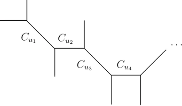
with toric diagram as in the following figure (4). That is, only two curves in X are allowed to intersect at any point. Hence, we exclude cases where three curves meet at one point in X, etc. With this restriction, we can introduce an ordering on the curves in X:

Cu2

Cu4

. . . Cu1

Cu3

Figure 4: X containing a string of curves.

Define a function

sgn:H2(X,Z)−→ {1,−1}

so that sgn(C) = 1 if NC/X ∼=O(−1)⊕ O(−1), andsgn(C) =−1 otherwise.

With these conventions, we can now state our conjecture on intersection theory.

Definition 2 Let X be a noncompact toric Calabi-Yau threefold such that dimH4(X,Z) = 0,

and suppose _NC ∼= O(−1)⊕ O(−1) or NC ∼= O ⊕ O(−2) ∀ C ∈ H2(X,Z). Then the classical

intersection numbers for X are given by

Kabc =

1 2

C /∈A

sgn[Cabc] + [C] , (4.31)

where the sum is taken in homology, and

[Cabc] = [Cua] +

Cua<Cα<C_ub

[Cα] + [Cub] +

C_ub<Cβ<Cuc

[Cβ] + [Cuc].

The sum is taken away from the set

A=_{[Cua],[Cub], . . . ,[Cua +Cua+1], . . .}.

This formula can be most simply understood as follows. The curve of minimum volume con-taining all three curves Cua, Cub and Cuc can be represented by the homology class

[Cabc] = [Cua] +

Cua<Cα<C_ub

[Cα] + [Cub] +

C_ub<Cβ<Cuc

[Cβ] + [Cuc].

Then each term of the sum [Cabc] + [C] corresponds to a curve in X containing Cabc.

Let us now apply this definition to a concrete case. Consider again the instanton part of the prepotential from example 1 above, equation (4.26):

Finst₌ n>0

ens

n3 +

en(s+t)

n3 −

ent

n3.

Then e.g.

∂3_Finst

∂s3 =

n>0

ens+en(s+t) .

Both the s curve and the s+t curve have normal bundle _O(₋1)_{⊕ O}(₋1) (this can be seen from the toric diagram, or directly from the vectors defining the secondary fan). Thus, each curve should have an intersection number equal to 1/2, which implies

Ksss=

1 2+

1 2 = 1.

By applying similar reasoning, we obtain the other intersection numbers

Ktss =Ktts = 1/2, Kttt= 0.

This intersection theory is also compatible with the flop X1 −→ X2 given above. We have also

verified that this prescription gives the simplest possible form for the extended Picard-Fuchs system on three parameter models of this type.

In fact, using the results of [18], we can argue that thus definition is the right one in general. In [18], it was shown that the Gopakumar-Vafa invariants for the spaces of interest are invariant under flops; this was done by considering a 3 parameter flop on the strip. The classical intersection numbers that preserve the polynomial part of the prepotential turn to be the ones given above, for the same 3 parameter models of [18]. Hence, this definition is the unique one in order to have a theory that transforms sensibly under flops.

4.4

Extended Picard-Fuchs System for

X

and

X

In this subsection, we derive an extended PF system under the assumption of the conjecture given in the previous subsection. First, we look at the example X1. In this case, we start from four

A-model Yukawa couplings:

Yttt := −

et

1−et +

es+t

1−es+t,

Ytts :=

1 2+

es+t

1₋es+t,

Ytss :=

1 2+

es+t

1₋es+t

Ysss := 1 +

es

1₋es +

es+t

The constant part of each Yukawa coupling is given by the conjecture, and the instanton (non-constant) part was taken from [18]. We repeat here the PF operators given by the standard toric construction of the mirror manifold ˆX1:

D1 = θ1(θ1 −θ2)−z1(2θ1 −θ2)(2θ1−θ2+ 1),

D2 = (2θ1−θ2)θ2−z2(θ1 −θ2)θ2,

D3 = θ1θ2−z1z2(2θ1−θ2)θ2. (4.33)

By solving (4.33), we obtain mirror mapss =s(z1, z2) andt =t(z1, z2). In particular, the Jacobian

of these mirror maps are written in terms of simple functions, as follows:

∂t ∂u1

= √ 1

1₋4z1

, ∂t ∂u2

:= 0, ∂s ∂u1

= 1 2

−1 + 4z1+√1−4z1

−1 + 4z1

, ∂s ∂u2

= 1, (4.34)

where ui = log(zi). With this data, we can compute the B model Yukawa couplings in ui

co-ordinates, and they turn out to be rational functions in zi whose denominators are given by the

divisor of the defining equation of discriminant locus of ˆX1:

dis( ˆX1) = (1−z2+z1z22)(1−4z1). (4.35)

The explicit results are given as follows:

Y111 = −

1 2

z1(−4z1+ 5−7z2+ 12z1z2 + 2z22−5z1z22+ 4z12z22)

(1₋z2+z1z22)(−1 + 4z1)2

,

Y112 = −

1 2

(1−2z1−z2+ 4z1z2−z1z22+ 2z21z22)

(1₋z2+z1z22)(−1 + 4z1)

,

Y122 = −

1 2

(−1 +z2+z1z22)

(1₋z2+z1z22)

,

Y222 =

1₋z1z22

1₋z2+z1z22

.

(4.36)

These results show that the conjecture given in the previous section is compatible with Conjecture 1 in Section 1. Therefore, we can construct an extended PF system by using the strategy outlined in Section 2. For brevity, we introduce here the following notation:

M_aα(t∗) :=

b

(Y_a−1(t∗))αb∂a∂bψ0. (4.37)

In the case of X1, we have two integrability conditions given in (2.7):

M1

1(t, s) =M21(t, s), M12(t, s) =M22(t, s), (4.38)

where we use the subscript 1 and 2 for t and s. By explicit computation, these two conditions turn out to be the same, and translated into a differential equation in zi variables by using (4.34)

and (4.36), we obtain:

(1 +z2+z1z22)D1+D2+z2D3

Next, we consider the second integrability condition given in (2.8):

∂1M11(t, s) =∂2M22(t, s), ∂2M11(t, s) = 0, ∂1M22(t, s) = 0. (4.40)

By explicit computation, we found that the second and the third conditions are translated into one rational differential equation:

θ2D1ψ0 = 0. (4.41)

The first condition is also translated into a rational differential equation but the result is very complicated. Now, we assert that (4.39) and (4.41) are a minimal set of extended PF operators for X1. The reason is the following. Let us consider the large radius limit of (4.39) and (4.41);

(θ2₁+θ1θ2−θ22)ψ0 = 0, (θ12θ2−θ1θ22)ψ0 = 0. (4.42)

These conditions are equivalent to the relations of the classical cohomology ring of X1:

k_t2+ktks−k2s = 0, k2tks−ktk2s = 0, (4.43)

which reproduces the conjectured triple intersection numbers, up to an overall scaling. From this fact, we can see that (4.39) and (4.41) give us a complete set of relations for the classical cohomology ring of X1 at the large radius limit. Since the PF equations are nothing but the

non-commutative version of the relations of the quantum cohomology ring of X1, which reduce to

relations of classical cohomology at the large radius limit, [14], we can propose the following set of differential operators as an extended PF system:

˜

D1 = (1 +z2+z1z22)D1+D2+z2D3,

˜

D2 = θ2D1. (4.44)

We checked that the solution space of (4.44) is given by,

1, t, s, ∂F ∂t ,

∂F

∂s, 2F −t ∂F

∂t −s ∂F

∂s C. (4.45)

Of course, we can derive the B-model Yukawa couplings (4.36) by using (4.44) as the starting point. An explicit example of this kind of computation will be given in Section 6 of this paper.

We can also construct an extended PF system of X2 in the same way asX1. Here, we briefly

present the data of this construction. The starting point is the A-model Yukawa couplings:

Y111 :=

es1 1−es1 −

es1+s2 1−es1+s2,

Y112 := −

1 2 −

es1+s2 1₋es1+s2

Y122 := −

1 2 −

es1+s2 1₋es1+s2,

Y222 :=

es2 1−es2 −

es1+s2

and the ordinary PF operators:

D1 := θ12−θ1θ2−z1(θ1+θ2)(θ1−θ2),

D2 := θ22−θ1θ2−z2(θ2+θ1)(θ2−θ1),

D3 := θ1θ2 −z1z2(θ1+θ2+ 1)(θ1+θ2). (4.47)

Let us introduce the logarithm of the B model coordinateszi.

u1 = log(z1), u2 = log(z2). (4.48)

By solving (4.47), we obtain the mirror mapss1 =s1(z1, z2) ands2 =s2(z1, z2) and their Jacobian:

∂s1

∂u1

= 1 2

(₋√1₋4z1z2−1 + 4z1z2)

(4z1z2−1)

, ∂s1 ∂u2

=₋1 2

(₋1 + 4z1z2+√1−4z1z2)

(4z1z2−1)

,

∂s2

∂u1

= ₋1 2

(₋1 + 4z1z2+√1−4z1z2)

(4z1z2−1)

, ∂s2 ∂u2

= 1 2

(₋√1₋4z1z2−1 + 4z1z2)

(4z1z2−1)

. (4.49)

With this data, we can compute the B model Yukawa couplings in ui_:

Y111 =

1 2z1

(5z1z2−2−12z1z22 + 7z2+ 4z32z1−5z22−4z21z22)

(z2−1 +z1)(4z1z2−1)2

,

Y112 =

1 2

(1₋z1−z2−z1z2−z2z12+z1z22+ 4z12z22+ 4z22z13−4z23z12)

(z2−1 +z1)(4z1z2−1)2

,

Y122 =

1 2

(1₋z2−z1−z2z1−z1z22+z2z12+ 4z22z12+ 4z12z23−4z13z22)

(z1−1 +z2)(4z2z1−1)2

,

Y222 =

1 2z2

(5z2z1−2−12z2z21 + 7z1+ 4z31z2−5z12−4z22z21)

(z1−1 +z2)(4z2z1−1)2

, (4.50)

and they turn out to be rational functions in zi whose denominators are divisors of defining

equation of discriminant locus of ˆX2:

dis( ˆX2) = (1−z1 −z2)(1−4z1z2). (4.51)

The derivation of the extended PF system by using the recipe in Section 2 proceeds in the same way as X1. In this case, we only have to consider

M₁1(s1, s2) =M21(s1, s2), M12(s1, s2) = M22(s1, s2), (4.52)

and

∂1M11(s1, s2) = ∂2M22(s1, s2), ∂2M11(s1, s2) = 0, ∂1M22(s1, s2) = 0. (4.53)

(4.52) gives us one differential equation for ψ0 with rational function coefficients in zi:

D1+D2+ (1 +z1+z2)D3

As for (4.53), the second and the third conditions give us a differential equations for ψ0:

(θ1−θ2)D3ψ0 = 0, (4.55)

and the first one gives us a complicated rational differential equation. For the same reasoning as

X1, we can propose an extended PF system for X2 as follows:

˜

D1 :=D1+D2+ (1 +z1 +z2)D3,

˜

D2 := (θ1−θ2)D3. (4.56)

We have also constructed an extended PF system for a three parameter space X3, in order to

further test the conjecture made in the previous section. Specifically, X3 satisfies dimH2(X,Z) =

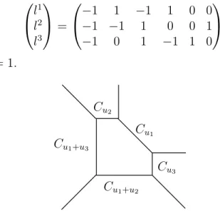
3, dimH4(X,Z) = 0, and is defined by the following vectors:





l1

l2

l3



= 



1 1 ₋1 ₋1 0 0 0 −1 −1 1 1 0 0 −1 1 0 −1 1



. (4.57)

The results are collected in Appendix A.

5

Adding open strings to

_O

(

₋

1)

_{⊕ O}

(

₋

1)

_→

P

.

So far, we have been able to demonstrate the existence of new differential operators which deter-mine mirror symmetry for noncompact toric Calabi-Yau manifolds which have no 4 cycle. One may also wonder what the applications are to the PF system derived for open mirror symmetry [24][10]. We will see that again, some modification of open string PF operators is necessary.

5.1

Review of open string geometry.

Recall [2][10] that open string mirror symmetry is a local isomorphism of moduli spaces (_X,_L) and ( ˆX,C); X and ˆX are Calabi-Yau manifolds which are mirror in the usual sense, and L ⊂X

is Lagrangian, while C⊂Xˆ is holomorphic. In the case at hand, (X,L) will be given by

Xr ={(w1, . . . , w4)∈C4−Z :|w1|2+|w2|2− |w3|2− |w4|2 =r}/S1,

together with either

Lr,c =Xr∩ {|w2|2− |w4|2 =c, |w3|2− |w4|2 = 0,

i

arg(wi) = 0} (5.58)

or

L′_r,c =Xr∩ {|w2|2− |w4|2 = 0, |w3|2− |w4|2 =c,

i

arg(wi) = 0}. (5.59)

There are then local moduli space isomorphisms (X,L)∼= ( ˆX,C), (X,L′₎∼_{= ( ˆX,C}′_{), where}

ˆ

Xz1 ={(u, v, y1, y2)∈C

2

Cz1,z2 = ˆXz1 ∩ {y

−1

2 y1=z2, y1 = 1}, (5.60)

C_z′1,z2 = ˆXz1 ∩ {y

−1

2 y1= 1, y1 =z2}. (5.61)

The detailed derivation of these spaces is given in [2]. One mathematical implication of open string mirror symmetry is that the geometry of ( ˆX, C) should determine the genus 0 open Gromov-Witten invariants of (X, L). This means that there should be functions defined on the moduli space ( ˆ_X,_C) which count holomorphic mapsf :D =_{z _∈C:_|z_{| ≤}1_{} →}X such thatf(∂D)_⊂L. Furthermore, in many cases such functions can be derived from an open string Picard-Fuchs system on ( ˆX, C). However, for the case at hand, it will be shown that the same sort of modification of the PF system, proposed for ordinary closed mirror symmetry, is also necessary in the open string setting.

We turn to the PF system on the moduli spaces ( ˆX,C) and ( ˆX,C′_).

5.2

Moduli space and Picard-Fuchs system for

( ˆ

X

,

C

)

.

From [10], we can define “open period integrals” on ( ˆ_X,_C) by

ΠΓ(z1, z2) =

Γ

dudvdy1dy2/(y1y2)

(uv+ 1 +y1+y2+z1y1y2−1)(y1−z2y2)(y1−1)

, (5.62)

Γ ∈ H4(C2 ×(C∗)2−X,ˆ Xˆ −C,Z). Then the derivations in [10] lead to a Picard-Fuchs system

for ( ˆ_X,_C), given as

D1 =θ1(θ1+θ2)−z1θ1(θ1+θ2), (5.63)

D2 =θ2(θ1+θ2)−z2θ2(θ1+θ2),

θi =zi

d dzi

;

these operators satisfy_DiΠΓ(z1, z2) = 0. This is exactly the noncompact PF system of the vectors

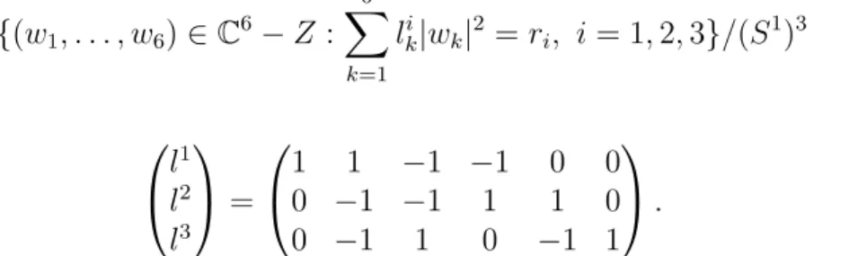
l1 _{= (1,1,−1,−1,0,0), l}2 _{= (0,1,0,−1,1,−1), and agrees with the results of [24].}

As was shown in [5], the solution space of {D1,D2} can be obtained, using the Frobenius

method, from a function

ω0(z, ρ) =

n≥0

c(n, ρ)zn1+ρ1

1 z

n2+ρ2

2 ,

where

c(n, ρ)−1 = Γ(1 +n1+ρ1)Γ(1 +n1+ρ1+n2+ρ2)Γ(1−n1−ρ1)∗

Γ(1₋n1−ρ1−n2−ρ2)Γ(1 +n2+ρ2)Γ(1−n2−ρ2).

According to [25], the solutions are expected to be

(1, t1, t2, W1, W2, . . .).

t1 and t2 give the open string mirror map, and this is trivial for the present example, so we have

Upon looking at the equations of (X, L), we can make the following geometric observation about a map f :D _→X with f(∂D) _⊂L. In the region where w3 =w4 = 0, L will intersect the

P1 of X; hence, such an f must obey f(D)_⊂P1. Then the natural interpretation of the variable

z2 is as a parameter controlling the size of a holomorphic disc D ֒→ X. It is therefore expected

that one of the double logarithmic solutions of (5.63) will look like

W1(z2) =

n>0

zn

2

n2, (5.64)

where the log terms have been disregarded due to ambiguity [2]. And indeed, it is the case that

W1(z2) = (∂ρ22ω0)|ρ=0.

The problem, though, is that (∂2

ρ2ω0)|ρ=0 is not a solution of (5.63). The easiest way to see this is to note that W1 is independent of z1, and (5.63) reduces toD2 = (1−z2)θ22 if z1 = 0.

The minimal resolution of this issue, which continues in the spirit of raising the power of PF operators, is to instead work with the system

{D1, θ2D2}. (5.65)

W1 is indeed a solution of these higher order operators.

A lingering difficulty, even after such a PF extension, is that (as will be shown below) there is expected to be another disc counting function

W2(z1, z2) =

n>0

(z1/z2)n

n2 ,

which measures the size of the “other disc”; that is, since L splits P1 into two discs, there should be a function corresponding to each disc. Functions with essential singularities such as W2 are

not allowed to be Picard-Fuchs solutions.

One way around this is to instead use the vectors l1_,−l2 _{to write down the noncompact PF}

system. Then it is easy to see that the resulting extended system

{D˜1, θ2D˜2}

will have solutions

˜

W1(z2) =

n>0

zn

2

n2, W˜2(z1, z2) =

n>0

(z1z2)n

n2 . (5.66)

These are the same as found in [26].

Similarly, we can perform calculations on the family ( ˆX, C′_{). This moduli space is given by}

vectors k1 _=l1_{, k}2 _{= (0,0,1,−1,1,−1), and the open string PF system we arrive at is}

D′1 =θ21−z1(θ1−θ2)(θ1+θ2),

Again, analogously to the above, let ω′

0 be the generator of solutions of {D′1,D′2}. Then there is

a disc counting function

∂_ρ22ω

′

0|ρ=0 =W′(z1, z2) =

n2>n1≥0

(−1)n1_(n

1+n2−1)!

(n1!)2(n2−n1)!n2

zn1

1 z

n2

2 (5.67)

which agrees with the result of [2]. Yet, once again we have the problem of this not being a solution of the given PF system; the same modification gives the system

{D′

1, θ2D2′}.

W′ _{is indeed among the solutions of this.}

The moral of this discussion is that the open string PF system, constructed in [24], is also incomplete in certain cases. Though the geometric meaning of raising the power of operators is less clear this time, we find that the same techniques are effective in open and closed string calculations. Moreover, the extension D2 → θ2D2 (rather than D1 → θ1D1) is the natural one.

This follows because z2 is the open string variable, and (∂ρ22ω0)|ρ=0 counts discs; hence, we must assure that the second partial derivative in ρ2 is a solution of the system.

Next, we will give an open string period integral definition for these degenerate situations.

5.3

Period integrals for

( ˆ

_X

,

_C

)

.

So far, it has been seen that the open PF system found in [24], which was later shown to be derived from a set of period integrals [10], does not always give the disc-counting functions one is interested in. Since local mirror symmetry on O(−1)⊕ O(−1) → P1yields an incomplete PF system, it is not so surprising that open strings on this same space should exhibit a similar failing. Hence, we need a definition of open string period integrals. For motivation, let’s review some geometric facts about ( ˆX,C). Let y be a local coordinate on Σ. Then following [2], we can think of the curve C as

Cz1,z2 = ˆXz1 ∩ {v = 0, y =z2} =C× {z2 ∈Σ}.

Then the coordinate on C ∼=C isu, and z2 parameterizes a family of curves in Σ.

Earlier, it was noted that the problem of period integrals was reducible to that of integrals on Σ. Here it is beneficial to make the same simplification. Notice that, when projected to Σ, the family of curves _{Cz1,y|y ∈ [z, z2]} becomes a real curve connecting z to z2. Hence, the sensible extension of Definition 1 to open strings is

Definition 3 Let X,ˆ Σ be as given in Definition 1, and C as above. Choose z, z2 ∈ Σ and

ˆ

γ _∈H1(Σ,{z, z2},Z). Then the open period integrals of ( ˆX,C) are defined to be

W(z1, z2) =

ˆ

γ

Resf=0

dy

1dy2/(y1y2)

f(z1, y1, y2)

.

For the purposes of the definition, z is considered to be fixed on Σ, andz2 is taken as a parameter.

ˆ

γ

ˆ

γ′

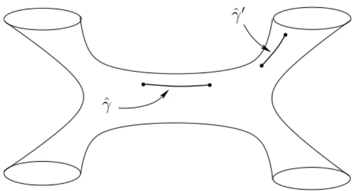
Figure 5: Real curves defining open string periods on Σ.

evaluation of these, and show agreement with the solutions of the proposed extended open string PF system of the last section.

There are two integrals, associated to the curves of the figure, and their calculation proceeds as follows.

W(z1, z2) =

ˆ

γ

logy1

dy2

y2

=

z2

z

log −1−y2 1 +z1y2−1

dy2

y2

=

n>0

(₋z2)n

n2 −

n>0

(₋z−1 2 z1)n

n2 ,

which is what we saw in the previous section from the PF system (after the rotationy2 →eiπy2). If

one is so inclined, the functions of (5.66) can be reproduced in the same way; this simply amounts to a change of the coordinate choices made in the mirror construction.

We also find

W′(z1, z2) =

ˆ

γ′

logy2

dy1

y1

=

z2

z

log−1−y1−

(1 +y1)2−4z1y1

2

dy1

y1

.

This integral is more difficult to directly evaluate, but as in [2] we can simply note that

z2

d dz2

W′ = log−1−z2−

(1 +z2)2−4z1z2

2 .

After Taylor expanding about z1 = 0 and integrating the result in z2, this matches (5.67).

6

More general local geometries.

We have come a long way toward a more complete picture of the differential equations governing local mirror symmetry. However, we have yet to test these ideas in the domain of applicability of [5]; namely, local Calabi-Yau manifolds KS, where S is a Fano surface and KS is its canonical

6.1

One 1-parameter example.

The simplest, though rather trivial, example is KP2 = O(−3) → P2. This can be defined as a symplectic quotient

KP2 ={(w₁, . . . , w₄)∈C4−Z :|w₁|2+|w₂|2+|w₃|2 −3|w₄|2 =r}/S1,

where Z ={w1 =w2 =w3 = 0}, r ∈R+ and theS1 action is given as

(w1, . . . , w4)→(eiθw1, eiθw2, eiθw3, e−3iθw4).

The original paper [5] associates a Picard-Fuchs system here, which is ultimately derivable from the period integrals of the mirror

ˆ

Xz ={(u, v, y1, y2)∈C2×(C∗)2 :uv+ 1 +y1+y2+zy1−1y2−1= 0}.

Again, from [17]:

ΠΓ(z) =

Γ

dudvdy1dy2/(y1y2)

uv+ 1 +y1+y2+zy1−1y2−1

for Γ _∈ H4(C2 ×(C∗)2 −X,ˆ Z) are the period integrals. Then we immediately recover the well

known PF operator

D =θ3+z(3θ)(3θ+ 1)(3θ+ 2), θ =z d dz,

whose solution space is generated by a functionω0(z, ρ) =n≥0c(n, ρ)zn+ρ. Here, the coefficients

can be written

c(n, ρ) = (Γ(1₋3n₋3ρ)Γ(1 +n+ρ)3)−1.

If we write the solutions in the variable t=∂ρω0|ρ=0, we get

Π = (1, t, ∂F/∂t)

Naturally, this implies that in the t variable, it must be the case that

D=∂t ∂3F

∂t3

−1

∂_t2.

Then, we can again give a ‘compactified’ operator

∂tD

which possesses a completed set of solutions. It is actually equivalent to just work with

θD=θ(θ3+z(3θ)(3θ+ 1)(3θ+ 2))

6.2

Completing mirror symmetry for Hirzebruch surfaces.

One parameter spaces of typeKS have already been exhausted, by theKP2 case. We will now turn to the two parameter spaces, namely the canonical bundle over the Hirzebruch surfacesF0, F1, F2.

As is well-known [5], the instanton part of the double log solution of the standard PF system is given by a linear combination of the ∂Finst.

∂ta . This fact tells us that the standard PF system of KS already includes the information coming from Ya−1(t∗) in (2.6). Therefore, we can take a

short cut in the process of constructing an extended PF system on KS. Examples of this explicit

construction will be given in the next subsection.

The symplectic quotient description is given byKFn =

{−2|w1|2+|w2|2+|w3|2 =r1n, (−2 +n)|w1|2−n|w2|+|w4|2 +|w5|2 =rn2}/(S1)2

where (w1, . . . , w5)∈C5−Zn. That is, the vectors in the secondary fan are

l1

n

l2

n

=

−2 1 1 0 0

−2 +n −n 0 1 1

.

The methods of [5] lead to PF operators:

KF0 :

D10 =θ12−z1(2θ1+ 2θ2)(2θ1+ 2θ2+ 1),

D02 =θ22−z2(2θ1+ 2θ2)(2θ1+ 2θ2+ 1)

KF1 :

D11 =θ1(θ1 −θ2)−z1(2θ1+θ2)(2θ1+θ2+ 1),

D1

2 =θ22−z2(2θ1+θ2)(θ1 −θ2)

KF2 :

D2

1 =θ1(θ1−2θ2)−z12θ1(2θ1+ 1),

D2

2 =θ22 −z2(2θ2 −θ1)(2θ2−θ1+ 1).

For each respective system, we lettn

1, tn2 be the logarithmic solutions. Each case comes equipped

with a single double log solution Wn. If ωn is the generating function of solutions on KFn and Πn

ij =∂ρi∂ρjω

n_|

ρ=0, then we can write these as

W0 = Π012, W1 = Π111+ 2Π112, W2 = Π211+ Π212.

Taking _Fn for the prepotential on KFn, we have the following equalities:

Wn = 2

∂_Fn

∂tn

1

+ (2₋n)∂Fn

∂tn

2

.

By a comparison of power series, we can demonstrate that the Πn

ij contain all the information

necessary to derive the (instanton part of) the prepotential on KFn. We find

Πn

11

Πn

12

=

0 4

2 ₋3n+ 2

∂Fn/∂tn1

∂_Fn/∂tn2

. (6.68)

The equality above holds at the level of instanton parts ofFn. We will now investigate the classical