Flow visualization through particle image
velocimetry and computational fluid dynamics in realistic model of rhesus monkey's upper airway
金, 智雄
http://hdl.handle.net/2324/1937186
出版情報:九州大学, 2018, 博士(工学), 課程博士 バージョン:
権利関係:
Flow Visualization
through Particle Image Velocimetry and Computational Fluid Dynamics in realistic model of rhesus monkey’s
upper airway
Ji-Woong KIM
A thesis for the degree of Doctor of Philosophy
Interdisciplinary Graduate School of Engineering Science
Kyushu University Japan April 2018
This thesis was reviewed and approved by the following:
Kazuhide Ito Professor
Department of Advanced Environmental Science and Engineering Faculty of Engineering Sciences
Kyushu University Thesis Adviser Chair of Committee
Masayuki Anyoji Associate Professor
Department of Advanced Environmental Science and Engineering Faculty of Engineering Sciences
Kyushu University
Taro Handa Professor
Department of Advanced Science and Technology Toyota Technological Institute
Thesis Summary
Individuals spend an increasing amount of time indoors leading to increased exposure to indoor air pollutants. It is necessary to clarify the detailed mechanism of inhalation exposure through airway. Inhalation toxicology studies and the development of respiratory drug delivery systems require biological testing by animals. However, the measurements by in vivo have many limitations owing to the complicated structure and small size of the nasal passage. Further, in vivo studies involving mammal surrogate models for inhalation toxicology studies have severe restrictions owing to ethics and protection.
In this study, I conducted an in vitro experiment and numerical prediction to investigate the flow distribution in the realistic geometry of a monkey airway as a representative surrogate mammal for test animals. in vitro experiment and numerical prediction models (in silico) were reproduced from CT data of an actual monkey airway for a 6-month-old male monkey whose scientific name is Macaca fascicularis and weighs 1.2 kg. Detailed measurements from the Particle Image Velocimetry (PIV) technique, as well as the numerical simulation through Computational Fluid Dynamics (CFD), are challenging in the understanding of
2
respiratory system. The purpose of the study included visualizing flow inside an upper airway with a complicated geometry.
PIV measurements of the in vitro provide an effective alternative to defining the flow patterns in realistic replicas of airway. PIV measurement was conducted under the oral and nasal inhalation condition. The numerical simulation was validated successfully using the observed 2D-PIV results. These results of measurement display the detailed mechanism of inhalation exposure of the physical behaviors. This study provides additional contributions in validating the use of CFD analyses to understand and predict monkey airway flows.
The contents of each chapter are summarized below,
Chapter1 introduce the necessary of clarify the detailed mechanism of inhalation exposure in airway for target monkey instead of the human. And objectives and organization of the dissertation.
Chapter 2 describes the PIV experiment method and the results of this study.
The results of PIV measurements at the 3D replica silicon model of a monkey airway then are showed using the 2-dimensional plane. A principles and applications of the basic PIV system is given in this chapter. The build-up procedure of the realistic model is described explicitly. The main content are described in this chapter on flow types, seeding, illumination, imaging, repetitive
correlation analysis, post-processing and result interpretation, with reference to experimental situations.
In Chapter 3, numerical methodology and turbulence model in use to the target airway monkey model is describes. For the grid independence study, the adequacy of grid resolution is tested by verifying fluid result with scalar velocities of PIV experimental result. In this chapter, four levels of grid resolution is adopted (4 million, 6 million, 8 million and 10 million total mesh cells with 10 prism layers). Hence the monkey airway geometry in case of 10 million total meshes is sufficient for predicting accuracy in this study.
In chapter 4, CFD prediction of airflow pattern in monkey airway model is compared with PIV experimental results using the monkey airway which has 10 million total mesh (in chapter 3). This analyses performed in this study use the Abe- Nagano - Kondoh model (LR-ANK) of low Reynolds number k-ε. The airflow field under isothermal condition is visualized using velocity vector map and profile. This chapter aims to provide data with insight into the characteristic of
flow patterns.
Chapter 5 describes conclusion, recommendations and future work for all content in this dissertation.
4
ACKNOWLEDGEMENTS
Firstly, I would like to express my sincere gratitude to my advisor Professor Kazuhide Ito for the continuous support of my doctoral studies and related research, for his great support, patience, motivation, enthusiasm, and immense knowledge. During the doctoral course, Prof.
Ito encouraged, supported, and believed in me while actively steering my research. Without his guidance and encouragement, it would not have been possible to complete the research and finish writing my dissertation.
In addition to my advisor, I would like to thank the rest of my thesis committee: Prof. Taro Handa of Toyota Technological Institute and Prof. Masayuki Anyoji of Kyushu University, for their insightful comments and encouragement, but also for the hard questions which motivated me to widen my research to incorporate various perspectives.
Special thanks go to my colleague Dr. Nguyen Lu Phuong, who provided me with the tools that I needed to choose the right direction and successfully complete my dissertation. Without his precious support it would not have been possible to conduct this research.
I wish to acknowledge my lab members for their assistance and intellectual engagement:
Dr. Yoo Sung-Jun, Dr. Chung Ju-Yeon, Alicia Murga and Kang Yu-Jin.
I would like to thank my family: my parents and my brother Noah for supporting me spiritually when I was writing my dissertation and for supporting me in life in general.
Last but not least, I would like to give my great appreciation of Ah-Reum - my wife. I couldn't have finished my PhD without her deep dedication and belief. Many thanks for leading me to come over hopelessness and loneliness with her meticulous care and considerations in every possible way. To my daughter, she is not born yet but already a part of my very soul and a motivation for me to accomplish this work.
CONTENT
Chapter 1 INTRODUCTION
1.1 MOTIVATION ... 1
1.2 OBJECTIVES ... 3
1.3 ORGANIZATION OF THE DISSERTATION ... 5
REFERENCE ... 7
Chapter 2 PARTICLE IMAGE VELOCIMETRY USING 3D REPLICA MONKEY AIRWAY MODEL 2.1 PIV PRINCIPLE ... 9
2.2 3D REPLICA MONKEY AIRWAY MODEL ... 15
2.3 PIV APPARATUS AND EXPERIMENTAL PROCEDURES ... 16
2.3.1 Creation of a 3D silicon model ... 16
2.3.2 PIV measurement setup ... 18
2.4 RESULTS AND DISCUSSIONS ... 24
2.4.1 The case of PIV experiment ... 24
2.4.2 Uncertainty analysis of PIV measurements ... 26
2.4.3 Velocity vector map and profile obtained by PIV technique ... 30
2.4.4 Conclusion and discussions ... 44
REFERENCE ... 47
Chapter 3 NUMERICAL STUDY OF AIRFLOW PATTERN IN MONKEY AIRWAY MODEL 3.1 NUMERICAL ANALYSIS OF FLOW FIELD... 49
3.1.1 Numerical methodology... 49
3.1.2 Selection of turbulence model ... 54
3.2 NUMERICAL SETUP ... 66
3.2.1 Grid design ... 66
3.2.2 Inflow boundary profile prescription for numerical simulation of oral and nasal airflow ... 73
3.2.3 Grid independence ... 74
3.3 CONCLUSION AND DISCUSSIONS ... 75
REFERENCE ... 77
Chapter 4 VALIDATION FOR NUMERICAL SIMUATION AND AIRFLOW PATTERN IN MONKEY AIRWAY MODEL
4.1 VALIDATION FOR NUMERICAL SIMULATION USING PIV RESULTS ... 79 4.2 COMPARISON OF CFD ANALYSIS RESULTS AND PIV EXPERIMENTAL
RESULTS... 84 4.3 CONCLUSION AND DISCUSSIONS ... 89 Chapter 5 CONCLUSION, RECOMMENDATIONS AND FUTURE WORK
5.1 CONCLUSION ... 91 5.2 RECOMMENDATION AND FUTURE WORK ... 94
CHAPTER 1
INTRODUCTION
1.1 MOTIVATION
The respiratory system is constantly being exposed to the various gases, harmful or not, contained in the ambient air, making its study an essential starting point in terms of human health and risk assessment due to inhalation. Due to the fact that the nose is a common site for particle deposition (AndersenⅠ et al., 1982; Brain JD et al., 1979; Hounam RF et al., 1977; Lippman M., 1970; Proctor DF et al., 1987; Swift DL., 1981), and the absorption site of many gases and vapors (Aharonson EF et al., 1974; Brain JD et al., 1979; Morgan MS et al., 1977; Stott WT et al., 1984), this organ has the wide potential to be harmed by inhaled irritants – e.g ozone, formaldehyde, and sulfur dioxide (Buckley LA et al., 1984; Harkema JR., 1987; Monticello TM et al., 1987; Walker D., 1983). The protective function of the
respiratory system makes it also vulnerable to several health risks, deriving in concerns for life quality management. In this instance, it becomes crucial to clearly define the detailed mechanisms of inhalation exposure through the airways for a deep understanding of phenomena like particle transport, deposition and mass transfer. Inhalation toxicology studies
and the development of respiratory drug delivery systems require biological animal testing.
In order to estimate human inhalation from animal inhalation in a toxicology study, an acceptable extrapolation formula is required to indicate the relationship between animal and human body sizes and inhalation mechanisms. Fundamental information such as the analysis of the flow field created inside the airways is needed for further studies. Thus, previous studies have analyzed human models as well as other mammals models, such as rats, mice, dogs, and monkeys, to predict convective mass transfer characteristics for upper respiratory tracts and other fluid initiated parameters(Inthavong et al., 2014; Ito et al., 2016; Wen et al., 2008). Typically, rats, rabbits, and dogs have much more complex turbinate structures than primate mammals such as monkeys and humans (Carey et al., 2007). Based on monkey and human anatomical and physiological information, monkeys have been used as surrogate mammals for humans in inhalation toxicology studies due to the strong similarities between both respiratory tract structures at a gross and microscopic level(Corley et al., 2012; Hislop et al., 1984; Kepler et al., 1998; Martonen et al., 2001; Monticello et al., 1989).
However, the only previous attempt to investigate fluid flow in rhesus monkeys was done by Morgan et al. (1991) who observed flow patterns through dye-water transport in hollow acrylic molds of the rhesus monkey’s nasal airways. Though the dye-water studies can provide qualitative information about the flow characteristics, they provide limited details of velocity data.
In this study, therefore, a monkey airway model that maintains most of the geometrical characteristics of respiratory structures from CT data of an actual monkey airway (6-month- old male, weight of 1.2 kg) has been developed. Then, an in vitro experiment to investigate the flow distribution in the realistic monkey airway geometry as a representative surrogate mammal for animal testing was conducted. The results of flow patterns in a realistic respiratory tract model using the Particle Image Velocimetry (PIV) technique, a 3- dimensional printer, and refraction control technique are hereby described.
The numerical simulation through Computational Fluid Dynamics (CFD) has been validated using the PIV experimental results. In addition, the visualization of flow inside the upper airways with a complicated geometry has been included. The experimental and numerical analyses have been conducted under oral and nasal inhalation conditions. The numerical simulation was validated successfully using the observed 2D-PIV results. These results of measurements show the detailed mechanisms of flow patterns. This study provides additional contributions in validating the use of CFD analysis to understand and predict monkey airway flows.
1.2 OBJECTIVES
The main objective of this dissertation aims to visualize results of Particle Image Velocimetry and numerical simulations in a realistic monkey airway model using various flow rates.
First target – Particle Image Velocimetry (PIV) for measuring airflow patterns of a monkey’s upper airway
The great advantage of the PIV technique is that it indicates high resolution of flow velocity vector information of a whole plane in the flow field at one time and obtains instantaneous velocity information and patterns (2 or 3-dimensional). It has therefore mainly been used to study the structure of turbulent flow fields using instantaneous flow field information and experimentally induced flows, such as water flow in the limited area or around streamlined objects (air flow around wing profiles and plane models, etc.). In this study, a PIV experiment has been conducted to investigate the fluid flow patterns of the monkey upper airway by using transparent, realistic replica model with a working fluid instead of air.
Second target – Computational fluid dynamics (CFD) analysis validated by the PIV experimental results
Computational fluid dynamics (CFD) is a computerized method to predict airflow by using numerical methods and algorithms. For the numerical simulation, The Low Reynolds type k-ε model (Abe-Kondoh-Nagano type) was selected in terms of turbulence to consider viscous sub- layer on the near wall space. The CFD results were validated by using PIV experimental results.
The calculation in flow field was very challenging due to the complex geometry that has highly curved and narrow spaces in bifurcation/separation zones as it includes the nasal/oral cavity, pharynx, larynx until the trachea.
1.3 ORGANIZATION OF THIS DISSERTATION
Chapter 1 introduces the necessity of clarifying the detailed mechanisms of inhalation phenomena inside the airways in order to extrapolate monkey model information into human scale. It also includes the objectives and organization of this dissertation.
In Chapter 2, the PIV experimental method and its results were described. The velocity distribution of PIV experimental data in the 3D replica silicon model of a monkey airway are then shown using a 2-dimensional plane. The principles and applications of the basic PIV system are given in this chapter. The build-up procedure of the realistic model is described explicitly. The main contents are flow types, seeding, illumination, imaging, repetitive correlation analysis, post-processing and result interpretation, with reference to experimental situations.
In Chapter 3, numerical methodology and turbulence model that were used in the target airway monkey model are described. The adequacy of grid resolution was confirmed through five levels of grid resolution (4 million, 6 million, 8 million, 10 million and 12 million total mesh cells with 10 prism layers) to ensure prediction accuracy and efficient calculation time.
Hence, the monkey airway geometry in case of 10 million elements mesh with 10 prism layers was considered to be sufficient in this study.
In chapter 4, CFD prediction of airflow patterns in the monkey airway model was compared with PIV experimental results using the case of the 10 million total mesh with 10 prism layers described in Chapter 3. The analyses performed in this study used the Abe- Nagano - Kondoh model (LR-ANK) of low Reynolds number k-ε type. The airflow field under isothermal conditions was visualized using velocity vector maps and profiles. This chapter aimed to provide data with insight into the characteristic flow patterns and the validation using PIV experimental data.
Chapter 5 concludes by summarizing significant outcomes from each research section between Chapters 2 to 4. The final part of this chapter highlight the potential contribution of this study and provide recommendations for further work.
Reference
1-1) AndersenⅠand Proctor DF. The fate and effects of inhaled materials. In: the nose:
Upper airway Physiology and the Atmospheric Environment. Elsevier Biomedical Press, Amsterdam, pp. 423-455. 1982.
1-2) Brain JD and Valberg PA. Deposition of aerosols in the respiratory tract. Am. Rev.
Respir. Dis. 123:1325-1373. 1979.
1-3) Hounam RF and Morgan A. Particle deposition. In: Respiratory Defense Mechanisms, J. D. Brain, DF Proctor, and LM Reid (eds). Marcel Dekker, NY, pp.125-126. 1977.
1-4) Lippman M. Deposition and clearance of inhaled particles in the human nose. Ann.
Otol. Rhinol. Laryngol. 79: 519-529. 1970.
1-5) Proctor DF, AndersenⅠ, Adams GK, and Man SFP. Nasal mucociliary function in man. In: Respiratory Tract Mucus, Ciba Foundation Symposium 54 (new series), Elsevier/North Holland, Amsterdam, pp. 219-234. 1987.
1-6) Swift DL. Aerosol deposition and clearance in the human upper airways. Ann.
Biomed. Engl. 9:593-604. 1981.
1-7) Aharonson EF, Menkes H, Gurtner G, Swift DL, and Proctor DF. The effect of respiratory airflow rate on the removal of soluble vapors by the nose. J. Appl. Physiol.
37: 654-657. 1974.
1-8) Morgan MS and Frank R. Uptake of pollutant gases by the respiratory system. In:
Respiratory Defense Mechanisms, JD Brain, DF Proctor, and LM Reid (eds). Marcel Dekker, NY, pp. 157-189. 1977.
1-9) Stott WT and McKenna MJ. The comparative absorption and excretion of chemical vapors by the upper, lower, and intact respiratory tract of rats. Fundam. Appl. Toxicol.
4: 594-604. 1984.
1-10) Buckley LA, Jiang XZ, James RA, Morgan KT, and Barrow CS. Respiratory tract lesions induced by sensory irritants at the RD50 concentration. Toxicol Appl.
Pharmacol. 74: 417-429. 1984.
1-11) Harkema JR, Plopper CG, Hyde DM, St. George JA, Wilson DW, and Dungworth DL. Response of the macaque nasal epithelium to ambient levels of ozone: A morphologic and morphometric study of the transitional and respiratory epithelium.
Am. J. Pathol. 1128: 29-44. 1987.
1-12) Monticello TM, Morgan KT, Everitt JI, and Popp JA. Effects of formaldehyde gas on the respiratory epithelium in the rat. Am. J. Anat. 169: 31-43. 1987.
1-13) Walker D. Histopathology of the nasal cavity in laboratory animals exposed to cigarette smoke and other irritants. In: Nasal Tumors in Animals and Man, Vol. Ⅲ, G Reznik and SF Stinson (eds). CRC Press, Boca Raton, FL, pp. 115-135. 1983.
1-14) Inthavong, K., Shang, Y., Tu, J. Surface mapping for visualization of wall stresses during inhalation in a human nasal cavity. Respir. Physiol. Neurobiol. 190, 54–61.
https://doi.org/10.1016/j.resp.2013.09.004. 2014
1-15) Ito, K., Mitsumune, K., Kuga, K., Phuong, N.L., Tani, K., Inthavong, K. Prediction of convective heat transfer coefficients for the upper respiratory tracts of rat, dog, monkey, and humans. Indoor Built Environ. 26, 828–840.
https://doi.org/10.1177/1420326X16662111. 2016.
1-16) Wen, J., Inthavong, K., Tu, J., Wang, S. Numerical simulations for detailed airflow dynamics in a human nasal cavity. Respir. Physiol. Neurobiol. 161, 125–35.
https://doi.org/10.1016/j.resp.2008.01.012. 2008.
1-17) Carey, S.A., Minard, K.R., Trease, L.L., Wagner, J.G., Garcia, G.J.M., Ballinger, C.A., Kimbell, J.S., Plopper, C.G., Corley, R.A., Postlethwait, E.M., Harkema, J.R. Three- Dimensional Mapping of Ozone-Induced Injury in the Nasal Airways of Monkeys Using Magnetic Resonance Imaging and Morphometric Techniques. Toxicol. Pathol.
35, 27–40. https://doi.org/10.1080/01926230601072343. 2007
1-18) Corley, R.A., Kabilan, S., Kuprat, A.P., Carson, J.P., Minard, K.R., Jacob, R.E., Timchalk, C., Glenny, R., Pipavath, S., Cox, T., Wallis, C.D., Larson, R.F., Fanucchi, M. V., Postlethwait, E.M., Einstein, D.R. Comparative computational modeling of airflows and vapor dosimetry in the respiratory tracts of rat, monkey, and human.
Toxicol. Sci. 128, 500–516. https://doi.org/10.1093/toxsci/kfs168. 2012.
1-19) Hislop, A., Howard, S., Fairweather, D.V.I. Morphometric studies on the structural development of the lung in Macaca fascicularis during fetal and postnatal life. J. Anat 138, 95–112. 1984.
1-20) Kepler, G.M., Richardson, R.B., Morgan, K.T., Kimbell, J.S. Computer simulation of inspiratory nasal airflow and inhaled gas uptake in a rhesus monkey. Toxicol. Appl.
Pharmacol. 150, 1–11. https://doi.org/10.1006/taap.1997.8350. 1998.
1-21) Martonen, T.B., Katz, I.M., Musante, C. A Nonhuman Primate Aerosol Deposition Model for Toxicological and Pharmaceutical Studies. Inhal. Toxicol. 13, 307–356.
https://doi.org/10.1080/08958370117552. 2001.
1-22) Monticello, T.M., Morgan, K.T., Everitt, J.I., Popp, J. a. Effects of formaldehyde gas on the respiratory tract of rhesus monkeys. Pathology and cell proliferation. Am. J.
Pathol. 134, 515–27. https://doi.org/10.1097/00043764-199004000-00003. 1989.
1-23) Morgan, K.T., Kimbell, J.S., Monticello, T.M., Patra, A.L., Fleishman, A. Studies of inspiratory airflow patterns in the nasal passages of the F344 rat and rhesus monkey using nasal molds: Relevance to formaldehyde toxicity. Toxicol. Appl. Pharmacol. 110, 223–240. https://doi.org/10.1016/S0041-008X(05)80005-5. 1991.
CHAPTER 2
PARTICLE IMAGE VELOCIMETRY USING 3D REPLICA MONKEY AIRWAY MODEL
This chapter describes the PIV experiment method and the results of this part of the study. The results of PIV measurements at the 3D replica silicon model of a monkey airway are then shown using a 2-dimensional plane. The principles and applications of the basic PIV system are given in this chapter and the build-up procedure of the realistic model is described explicitly. The main contents hereby described are flow types, seeding, illumination, imaging, repetitive correlation analysis, post-processing and result interpretation, with reference to experimental situations.
2.1 PIV PRINCIPLE
PIV technique has been developed to measure flow field of scalars and vectors in the experimental fluid from the 1980’s (Adrian 1991). The great advantage of PIV technique are
that it indicate high resolution flow velocity vector information of a whole plane in the flow field in one time and obtain instantaneous velocity information and 2 or 3-dimensional flow pattern of velocity information. It has therefore mainly been used to study the structure of
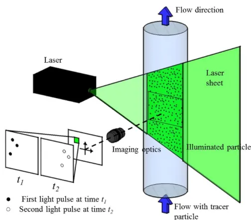
Figure 2.1 Diagram of PIV conceptual diagram
turbulent flow fields using instantaneous flow field information (Westerweel, 1996;
Haigermoser, 2008) and the experimentally induced flows, such as water flow in the limited area or around streamlined objects, air flow around wing profiles and plane models, etc. (Adrian 1991; Stanislas et al. 2000). PIV techniques can be characterized as an optical method of flow visualization that measures the displacement of tracer particles that in the experimental fluid due to its non-intrusive character.
Using a high-speed digital camera, the particle moving is captured by capturing scattered light from the individual particles. The local velocity of a flow field is determined by the micro- linear distance and direction in which the tracer particles passing through a certain point move
during the minute time interval. The displacement of particle in the target region is calculated by captured successive images. To approximate u velocity of x-component and v velocity of y- component to the actual flow velocity, the displacement of particle must be sufficiently small.
In other words, the trajectory drawn by the particles must be guaranteed to be linear and isotropic. PIV conceptual diagram is shown in Figure 2.1. u and v is expressed by following equation 2.1.
2 1 2 1
2 1 2 1
2 1 2 1
lim , lim
t t t t
x x x y y y
u v
t t t t t t
... (2.1)
The captured PIV images are analyzed by divided image into a grid of interrogation areas that is smaller sub-areas. Then, a displacement vector for the tracer particles is detected in each interrogation area by using the cross-correlation statistical calculation. The process is repeated on each next interrogation area until reaching the last interrogation area. The single exposure frame is used to measure the single exposed image pairs between successive frames, by means of cross-correlation. The objective of the method is to locally find the best match between the images in a statistical sense (Figure 2.2). The correlation function RII requires the evaluation of the following equation 2.2 (Raffel et al, 2007):
( , ) ( , ) '( , )
K L
II
i K j L
R x y I i j I i x j y
... (2.2)where I(i, j) represents the intensity value for the (i, j) pixel. This function statistically measures the degree of correlation between two samples I and I' for a given shift (x, y). The shift position where the pixel values align with each other gives the highest cross-correlation value, and this represents the average displacement of the particles in a given interrogation window. A high cross-correlation peak is identified when a particle match up with its corresponding shifted partner, and low cross-correlation peaks may be observed when single particle match up with surrounding particles. The former correlation is correct correlation, and the latter one is called random correlation or undesired correlation. If the shift of each particle is stable then the correct correlation produce a peak value that must be higher than the noise peaks produced by the random correlations. The height of the main peak relates to the number of particle pair correlations and hence to the signal to noise ratio. Seeding particles entering or leaving the interrogation area between the recording of the first and the second image, will not contribute to the true correlation. They do contribute to the random correlations that make decrease the signal-to-noise ratio. This phenomenon is called as “loss-of-pairs” or “signal drop-out”.
Determination of the location of the peak value is the key factor to define displacements precisely. RII can be decomposed into the following components
C P F
II D D
R R R R R R ... (2.3)
RC is the convolution of mean image intensity, RP is the pedestal component resulting from each
particle image correlating with itself, and RF is the fluctuating component resulting from the correlation between fluctuating image intensity with mean image intensity (Adrian, 1988). The positive and negative displacement components are RD+ and RD-, respectively (see Figure 2.3).
The signal used to measure displacement is contained only in the RD+ component. Contributions from all other components of the correlation function may bias the measurements, add random noise to the measurements, or even cause erroneous measurements. Therefore, it is desirable to reduce or eliminate as much as possible the other components. In practice, to efficiently compute the correlation plane, Fourier transform processing is adopted in PIV. A camera image may be considered a two-dimensional signal field analogous to a one-dimensional time series.
Fast Fourier Transforms (FFT’s) are used to speed up the cross-correlation process. The FFT’s
cross-correlation method resulted in a single peak on the correlation plane that represented the average displacement of the particles in the window during the time delay between two frames.
Instead of performing a sum over all elements of the sampled region, the operation can be reduced to a complex conjugate multiplication of each corresponding pair of Fourier coefficients. The cross-correlation was then obtained by using the FFT’s algorithm in Equation 2.4 and 2.5:
,
,
,RII x y f x y g x y ... (2.4)
II
,
, * ,F R x y F u v G u v ... (2.5)
where F(u,v) and G(u,v) are the Fourier transforms of f(x, y) and g(x, y), * denotes a complex conjugate and F represents a Fourier transform. The cross-correlation could be computed become simpler and less computer expensive by taking the inverse Fourier transform of the product of the FFT’s of each of the interrogation areas. The position of the correlation peak was
then estimated to sub-pixel accuracy by using a Gaussian fit function.
In this part the basic principles of PIV have been introduced. The following section describes the PIV system and experimental practices used in this study.
Figure 2.2 Description of PIV system
Figure 2.3 Spatial cross correlation function
2.2 3D REPLICA MONKEY AIRWAY MODEL
To perform the PIV measurements, a monkey air way model was made from silicon. The present silicon model was developed from a 3D replica model of the monkey using computed tomography (CT) data. Figure 2.4 is shown the CT data. The subject monkey, Macaca fascicularis, was a 6-month-old male with a weight of 1.2 kg. Micro-CT imaging from the upper airway of the monkey including nasal and oral cavities and trachea were performed at a resolution of 200 μm. The original CT images were converted into a compatible file format by
using Mimics ®(Materialise NV) to generate and modify 3D surface models of medical images.
A surface model was generated from continuous 2D contour data by translating segmented, modified, and smoothed contour points into a data series that was loaded into ANSYS preprocessing software package ICEM-CFD (ANSYS Inc.). Additionally, ICEM-CFD was used to modify the surface mesh and create a volume mesh of the model with unstructured
tetrahedral elements (See figure 2.5). Surface geometries of the monkey respiratory tract were also exported as an STL file format. The monkey respiratory tract model possessed a length and inner surface area approximately corresponding to 1.05 × 10⁻¹ m and 2.81 × 10⁻⁵ m2, respectively. Table 2.1 lists the details of the monkey’s geometry.
Table 2.1 Details of the 3D replica monkey model by using the STL data.
Original data Scale-up 1.5 time data
Total inner surface area (m2) 2.81×10⁻⁵ 6.32×10⁻⁵
Total inner volume (m3) 1.27×10⁻⁵ 4.29×10⁻⁵
Total length (m) 1.05×10⁻¹ 1.58×10⁻¹
Maximum height excluding pipe (m) 4.32×10⁻² 6.48×10⁻²
Maximum width excluding pipe (m) 2.81×10⁻² 4.22×10⁻²
Area of right naris (m2)
/Equivalent diameter (m) 5.48×10⁻⁶/2.64×10-3 1.23×10⁻⁵/3.96×10-3 Area of left naris (m2)
/Equivalent diameter (m) 5.46×10⁻⁶/2.64×10-3 1.23×10⁻⁵/3.96×10-3 Area of mouth (m2)
/Equivalent diameter (m) 4.08×10⁻⁶/7.21×10-3 9.18×10⁻⁵/1.08×10-2 Area of trachea (m2)
/Equivalent diameter (m) 2.81×10⁻⁵/5.98×10-3 6.32×10⁻⁵/8.97×10-3
2.3 PIV APPARATUS AND EXPERIMENTAL PROCEDURES
2.3.1 Creation of a 3D silicon model
In order to create a 3D silicone model, a 3D respiratory tract model was created with a 3D
printer (CMET Inc., ATOMm-4000) by using the STL data. First, a negative model that represented the monkey’s upper airway was constructed from a water-soluble plastic. The lamination layer in the z-direction corresponded to 15 μm and the object resolution corresponded to 20 × 20 μm in the x- and y-direction. Following a precise and suitable surface
treatment of a negative model, the model was placed in a rectangular box, and transparent silicon material (TSR-833) was poured into the box. Finally, a plastic (a negative model in silicon material) was dissolved and flushed out by water to create a positive model that corresponded to a solid containing void space to reproduce the respiratory tract geometry with a transparent silicone material as shown in figure 2.6.
Figure 2.4 CT data of a real monkey airway using Mimics ®(Materialise NV)
Figure 2.5 Computational geometry and mesh of virtual airway
Figure 2.6 A silicone monkey airway model created by a 3D printer
In order to ensure the measurement accuracy of the PIV experiment, a silicone airway model that was 1.5 times larger than the actual size was created. This CT data was provided by third parties (Ina-Research Co.) and corresponds to secondary usage of in vivo data acquired in experiments conducted completely separately from this study.
2.3.2 PIV measurement setup
The PIV is a technique for measuring the velocities of tracer particle ensembles from images of particles captured at successive times by assuming that the particle movement is the same as the fluid motion. The instantaneous velocity field that plays an important role in the structure of turbulent flow fields is measured by using light scattered from tracer particles on an illuminated plane. In the PIV algorithm, the consecutive images are compared to calculate the particle displacement of the interested area. The two velocity vectors between pairs of frames at any point are determined by dividing the distance of displacement by the time delay. The analysis of the PIV images is conducted by dividing the single frame into an interrogation area
(IA) consisting of smaller sub-areas. A displacement vector for the tracer particles is detected in each IA by using a cross–correlation statistical method. All the fore-mentioned procedures are repeated in the next interrogation area until all areas of captured frames are completed. In the PIV measurement in the study, the visualization of the 2D flow field in the monkey upper airway was conducted by using silver-coated hollow glass spheres with a mean diameter of 10 µm as tracer (seeding) particles. The movement of tracer particles were captured by using a high-speed camera (Photron, Inc., FASTCAM SA4 model 500K-C1) and recorded on a complementary metal-oxide semiconductor (CMOS) sensor. The density of the hollow glass spheres corresponded to 1.4 g/cm3. The field of view in the CMOS camera was focused on the target region by illuminating a light sheet with a thickness of 3 mm discharged from the continuous wave (CW) laser. A CW laser (Beamtech Optronics, Diode-pumped solid-state green laser 2W) with a wavelength of 532 nm was used as the light source. The image data were analyzed with Dynamic studio 3.31. The frame rate was defined as 500 frames per second and 2000 frames per second based on the flow rate for the flow velocity at a full size corresponding to 1024 × 1024 pixels. Initially, the particle displacements were determined by using an interrogation size corresponding to 128 × 128 pixels. The vector fields were analyzed by using the cross–correlation method adaptive based on fast Fourier Transform (FFT) algorithms. The size of the initial interrogation area (IA) was set as 8 × 8 pixels with a 50%
overlap to satisfy the Nyquist criterion. The adaptive correlation method iteratively calculated velocity vectors with an initial IA of a size equal to N times the size of the final IA and used the
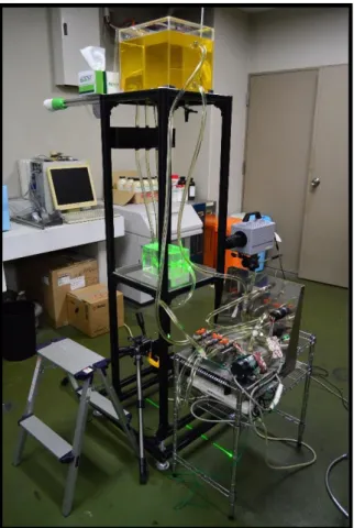
intermediary results as information for the next IA of a smaller size until the final IA size was reached. The spurious vectors on the vector field were removed by using velocity range, peak ratio, and local median filters. The vector statistics map was calculated by using 5456 velocity vector maps of an averaged velocity vector obtained from two consecutive images. Figures 2.7 show the experimental setup with the monkey airway model for the PIV system.
Figure 2.7 The experimental setup for PIV
The silicone material forming a positive model for a monkey upper airway and pure water possesses a different refractive index (RI). In order to capture particle motion by using a laser light sheet without refraction, it is necessary to match the refractive index of the silicone material with the working fluid. Because, if the light passes through different material, the refraction happen. Then we can’t get the correct image (See figure 2.8).
Figure 2.8 The action of refractions
In order to eliminate the refraction of laser sheet, we used water/sodium iodide mixture as working fluid. The Refractive index (RI) of the working fluid and silicon material model is matched with the naked eye. In the experiment, a 61/39 water/sodium iodide mass percentage mixture was used as a working fluid to match the RI of the flow of the working fluid and the silicone material constituting the monkey airway model. The refractive index of the NaI solution changed based on the temperature. With respect to a solubility of the NaI solution dependent on temperature, the PIV experiment was conducted at a constant temperature. The RI of the experiment was specified as 1.413. The gridline examination for matching the RI is shown in table 2.2.
Table 2.2 Refractive index matching using Grid line.
Water (ml)
Sodium Iodide(g)
(NaI)
Refractive index of aqueous Nai
solution
Picture Verification of Gridline
100 0 1.336
42 1.390
62 1.413
A liquid was used as a working fluid as opposed to air, and thus the Reynolds number should be the same based on the inhalation condition in real airflow in the numerical simulations as well as in the experimental measurements. Given that model is scaled by a factor of 1.5, the relationship is defined according to equation 2.6 and equation 2.7 as follows:
working fluid real
working fluid air
air silicone model
v L
V V
v L
... (2.6)
siliconemodel NaI
working fluid working fluid silicone model air
real air
L v
Q V A Q
L
... (2.7)
where Vworking fluid denotes the representative velocity in the trachea, Qworking fluid denotes the
volumetric flow rate, ν denotes the kinematic viscosity of the fluid, and L denotes the length
scale (m) of the trachea (Lsilicone model/Lreal=1.5). Additionally, A denotes the representative area (m2) of the trachea. The kinematic viscosity of the working fluid corresponds to νworking fluid = 0.712 × 10⁻⁶ m2/s as determined by using a Cannon-Fenske routine viscometer(See figure 2.9, table 2.3).
Table 2.3 Kinematic viscosity of NaI solution for PIV.
water 100ml, NaI 63g, refractive index 1.413, 20℃
20℃ Dropping time(s)
average of time
1 2 3
NaI aq 55.533 55.531 55.535 55.533
H2O 61.225 61.216 61.280 61.240
T(℃) μH2O (mPa·s) μH2O (kg/m·s)
15 1.140000 0.001140
16 1.110000 0.001110
17 1.083000 0.001083
18 1.056000 0.001056
19 1.030000 0.001030
20 1.005000 0.001005
μNaI 0.00091
ρNaI aq(g/cm3) ρNaI aq(kg/m3)
15.000 1.285 1284.800
19.300 1.282 1282.300
20.100 1.280 1279.587
νNaI aq(m2/s) 0.000000712
The density (ρworking fluid) corresponds to 1.28 × 10³ kg/m3, and the temperature of the working fluid and surrounding environment are maintained at 20℃ during the experiment. The flow rate of the working fluid on the trachea was controlled by using a flow control valve placed behind a high-pressure flowmeter (KOFLOC, model RK1400 with an accuracy of ±2%). In the experiment, the condition of the monkey upper airway model was reproduced for nasal and oral cavities by connecting a pump to the entrances of the oral and nasal cavities. The monkey upper airway model was inverted to control the inflow working fluid profile approaching nasal and/or oral cavities. Working fluid was supplied from the top to bottom, and the formation of fully developed working fluid profile in supplied tube was confirmed in the preliminary experiment.
2.4 RESULTS AND DISCUSSIONS
2.4.1 The case of PIV experiment
In order to measure PIV by using a 3D silicon monkey airway model, the case is divided into two parts under oral and nasal inhalation. With respect to the oral inhalation, the nasal cavity entrance (i.e., the nostril) was closed and vice versa. The flow rate of the working fluid (QNaI) ranged from 0.2826 L/min to 1.5544 L/min in accordance with the Reynolds number matching
Figure 2.9 The equipment for measurement of viscosity and density
of air flow rate, respectively. Table 2.4 shows the experimental cases of PIV measurement based on the Reynolds number setting.
Table 2.4 Cases of PIV measurements based on Reynolds number matching under seven types of oral and nasal inhalation conditions.
Qair
(L/min)
Qworking fluid
(L/min)
Vworking fluid
(m/s)
Vair
(m/s)
Reynolds number
(Re)
Nominal time constant (s)
Recording time (s)
4 0.2826 0.0745 2.3725 938 9.12 10.914
6 0.4239 0.1118 3.5587 1407 6.41 10.914
10 0.7066 0.1863 5.9312 2346 3.64 5.547
14 0.9892 0.2608 8.3037 3284 2.60 5.547
18 1.2718 0.3353 10.6762 4222 2.03 2.7285
20 1.4121 0.3725 11.8624 4692 1.84 2.7285
22 1.5544 0.4098 13.0486 5161 1.49 2.7285
The distance between the CMOS camera and illumination section with respect to the laser light sheet are considered to divide the target X-Y plane into two regions, namely the cavity and trachea regions as shown in figure 2.9.
In the cavity region, lines L1 and L2 were adopted for the oral inhalation condition and line L3 and L4 were adopted for the nasal inhalation condition to discuss the velocity profile of working fluid. In the trachea region, the visualized target region was consistent with respect to the oral and nasal inhalation conditions. The velocity profiles of the oral and nasal inhalation conditions were compared on lines L5 and L6 at the trachea region. The distances of the cross line (from L1 to L6) at the PIV measurements were normalized by dividing them
Figure 2.9 Visualized target region in 2-dimensional captured picture.
with the diameter of inlet (D). The non-dimensional distance was defined as dependent on the diameter of the cross line along the Y-axis, respectively. Individual non-dimensional distances were compared with different diameters of each cross line.
2.4.2 Uncertainty analysis of PIV measurements
In order to examine the PIV results, a preliminary PIV experiment was conducted to locate a suitable tracer particle by using particles of mean diameter (dp) corresponding to 10 µm and 60 µm under oral inhalation with an airflow rate of 10 L/min. The results indicated that the size of the tracer particles was of particular importance in the PIV measurement. Generally, the magnitude of the drag force increased with the frontal area of a sphere that impinges on the fluid, and it can influence particle movement. The density of the permeable tracer particle (dp
= 60 µm) was fairly identical to the working fluid density (ρ = 1.28 × 10³ kg/m3). The tracer (dp
= 10 µm) with a density of 1.4 × 10³ kg/m3 displayed a discrepancy of approximately 9%.
Gravitational settling velocity of the tracer particle (dp = 10 µm) as estimated by Stokes’ Law corresponded to 7.2 × 10⁻⁶ m/s. In a centrifugal force field, a centrifugal force deflects the tracer particle from the actual fluid flow in the flow in the bending tube. In figure 2.10, the branch has a tangential velocity component and a velocity component and has a radial velocity component [m/s]. The direction and force of gravity equilibrium do not move. The order of the settling velocities was considerably smaller than average convective velocity in the cavity and trachea, and these were negligible. It is also necessary to verify deflection by a centrifugal force acting on tracer particle as follows:
2
tan 1
18
t
r P P
t P
u
v d
u r
... (2.8)
where vr denotes settling velocity, and ut denotes representative fluid velocity. In the PIV measurement, the degree of deflections of rotational motion and particle motion (tan θ 4L/min, tan θ 10L/min and tan θ 20L/min) corresponded to 2.0 × 10⁻⁵, 4.6 × 10⁻⁵, and 9.2 × 10⁻⁵, respectively.
The values were reasonably small (tan θ < 0.01), and it was concluded that the tracer particle (dp = 10 µm) perfectly followed the motion of the working fluid.
Figure 2.10 Particle motion in a centrifugal field
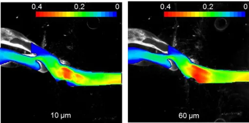
In order to visualize a flow pattern, PIV measurement was conducted using with tracer particles of mean diameter corresponding to 10 µm and 60 µm under oral inhalation of 10 L/min. The normalized scalar velocity in the trachea region is shown as figure 2.11. The tracer (dp = 10 µm) was coated with silver, and relatively definite visualization images were obtained. In case of the tracer (dp = 60 µm), an unstable distribution was observed because of the negative influence of the drag force in the fully developed fluid flow. Figure 2.12 shows a comparison of scalar velocity profiles with two upstream locations (line L5 and L6). The amplitudes of error bars correspond to the standard deviation of the measurements. On the near top surface, the drag force had a larger impact on the tracer (with dp = 60 µm) than on the tracer (with dp = 10 µm).
Figure 2.11 A flow pattern of normalized scalar velocity in the trachea region with tracer
particles of mean diameter corresponding to 10 µm and 60 µm by PIV under oral inhalation of 10 L/min.
Figure 2.12 Profile with standard deviation on line L5 and L6 under oral inhalation of 10 L/min
The velocity magnitude of tracer particle (dp = 60 µm) was smaller than the scalar velocity of the tracer particle (dp = 10 µm). The velocity of the tracer (dp = 60 µm) increased on the near bottom surface because the settling velocity influenced the velocity magnitude of the y- component. In this study, 10 µm tracer particle was adopted with respect to the following PIV experiments.
2.4.3 Velocity vector map and profile obtained by PIV technique
In order to classify the flow pattern as a function of Reynolds number, the results of seven fluid flow rates were compared based on the oral inhalation. The velocity values are calculated as scalar velocities by using two velocity components. Figure 2.13(A) shows the PIV results of the seven cases with scalar velocity at line L6 (see figure 2.9). The mean velocities at cross line L6 were normalized by using the outlet velocity as shown in figure 2.13(B)
( * *
2 2
/ out,
y y
U U U u v , u: velocity magnitude of x-component, v : velocity magnitude of y- component). The flow through the passageway was not sufficiently developed in cases involving 4 L/min and 6 L/min of the fluid flow rate. A gradual increase in the value of flow rate to 22 L/min (Re=5161) led to the flow becoming fully developed in the passageway. In the trachea region, the 10 L/min (Re=2346) flow rate was located in the transition zone.
Figure 2.13 Profiles of all conducted experimental result on line L6 (Figure. 2.9) based on the Reynolds number matching under oral inhalation.
2.4.3.1 Velocity map cavity region Oral inhalation condition
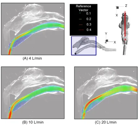
In this study, PIV results divided by cavity and trachea regions were compared in the cases involving fluid flow rates corresponding to 4 L/min, 10 L/min, and 20 L/min. The PIV measurement results of the velocity vectors and velocity distribution of the oral cavity region are shown in figures 2.14 and 2.15, respectively. Figure 2.14 shows the velocity vector map obtained using PIV at cross-section of oral cavity for the flow rates corresponding to (A) 4 L/min, (B) 10 L/min, and (C) 20 L/min. Fig 2.15 shows the two dimensional mean velocity distribution of oral cavity plotted at the vertical cross section A-A' of the mouth entrance center for the flow rates corresponding to (A) 4 L/min, (B) 10 L/min, and (C) 20 L/min. The bottom part of the oral cavity that segued into the trachea presents minute flow fields that appear to be stagnant. Figure 2.16 shows the velocity distribution with velocity vectors of trachea region under oral inhalation condition. The flow is characterized by the region of separated flow at the start of the nasal/oral cavity, pharynx, and larynx and down to trachea. The fluid flow in the oral cavity for the three cases is indicated by a similar flow structure and complicated flow patterns. An angle of the inflow boundary leads to the occurrence of recirculating flow in the vicinity of the mouth opening. In the recirculation zone, back flow and reattachment point is confirmed (see Fig. 2.17).
Figure 2.14 The velocity vector map obtained using PIV at cross-section of oral cavity
Figure 2.15 The contours of the time averaged velocity distribution obtained using PIV at cross-section of oral cavity
Figure 2.16 Contours of time averaged velocity distribution in the trachea with velocity vectors under oral inhalation condition (Cross-section C-C’ : center of trachea region)
(A) The recirculation zone and main stream at cross-section of oral cavity under 4 L/min
(B) Normalized scalar velocity profile and reattachment point
Figure 2.17 The recirculation zone and reattachment point at cross-section of oral cavity
Nasal inhalation condition
The PIV measurement results of the velocity vectors and velocity distribution of the nasal cavity region are shown in figures 2.18 and 2.19, respectively. Figure 2.18 shows contours of time averaged velocity distribution in the left nasal cavity with velocity vectors at cross-section A- A’ for the flow rates corresponding to (A) 4 L/min, (B) 10 L/min, and (C) 20 L/min. Figure 2.18
shows contours of time averaged velocity distribution in the right nasal cavity with velocity vectors at cross-section A-A’ for the flow rates corresponding to (A) 4 L/min, (B) 10 L/min, and (C) 20 L/min. The velocity distribution under a nasal inhalation condition with velocity vectors of the vertical cross section are plotted on cross section A-A' (left cavity) and B-B' (right cavity) by the center of the nostril. The velocity vectors were scaled to a common reference value to improve the clarity of the results. The PIV results do not indicate the same geometry in the left and right nasal cavities since the shape of nasal cavity is not symmetric. It was not possible to confirm the flow patterns of vicinal maxillary sinus because of the deposition of particles on the wall. However, the flow pattern in the region passing through the oral cavity to the pharynx was reliably obtained. A similar flow structure at the inlet was confirmed despite a difference in shape. The protruding part around the inlet changes the flow pattern abruptly. The velocity is reduced due to the interference of walls with complex shapes. The velocity increases again after the airflow moves into the pharynx area. Figure 2.20 shows the velocity distribution with velocity vectors of trachea region under nasal inhalation condition. The PIV results between oral and nasal inhalation are compared with a scalar velocity distribution of an outlet
Figure 2.18 Contours of time averaged velocity distribution in the nasal cavity with velocity
vectors at cross-section A-A’of left nasal cavity
Figure 2.19 Contours of time averaged velocity distribution in the nasal cavity with velocity vectors at cross-section B-B’of right nasal cavity
Figure 2.20 Contours of time averaged velocity distribution in the trachea with velocity vectors under nasal inhalation condition (Cross-section C-C’ : center of trachea region)
part that possesses the same geometry. The flow of nasal inhalation condition also is characterized by the region of separated flow at the start of the nasal/oral cavity, pharynx, and larynx and down to trachea. The velocity vector plots exhibited a similar flow structure in oral and nasal inhalation for all three flow rates. However, flow structural variations exist due to the
(A) The left nasal cavity under 4, 10 and 20 L/min
(B) The right nasal cavity under 4, 10 and 20 L/min
Figure 2.21 Observed flow structures on nasal vestibule in the monkey nasal airway.
inlet location to access trachea. After the fluid flow passes the converging path of pharynx, the velocity vector increases, and thus flow separation occurred with abrupt geometrical changes from the larynx to trachea.
2.4.3.2 Profile of Oral and Nasal cavities Profile of oral inhalation condition
In order to compare the profile of three flow rate, the mean velocities at each cross line were normalized by using the outlet velocity ( * *
2 2
/ out,
y y
U U U u v , u: velocity magnitude of x- component, v : velocity magnitude of y-component). Figure 2.20 shows the normalized velocity profiles for the three inspiratory flow rates that are plotted at two cross line locations for oral inhalation. As shown in Figure 2.22A, the normalized scalar velocity profiles of the line L1 indicates that the fluid on the upper (vicinal palate) side moves faster while the fluid on the lower (vicinal tongue) side moves slower. Hence, the deposition is expected to occur at the lower side of trachea with a weak velocity magnitude as shown in Fig 2.22A. Figure 2.22B shows the normalized velocity profiles for the three inspiratory flow rates at two cross line locations in trachea region. The fluid flow corresponding to 4 L/min exhibits a precipitous inclination of the velocity magnitude at the upper sides.
Figure 2.22 Profile of normalized scalar velocity in oral cavity and trachea region under oral inhalation.
Profile of nasal inhalation condition
The velocity magnitude of the line L2 in figure 2.9 corresponds to a developed convex profile.
In the case of line L2, normalized scalar velocities indicate a minute value near the bottom surface. The normalized velocity profiles for the three inspiratory flow rates are plotted at three cross line locations for nasal inhalations as shown in figure 2.9. As described above, the nasal cavity with unequal geometry exhibits different patterns in the flow field. As shown in figure
2.23A (left nasal cavity), a pronounced concave curve profile appears as indicated by the protruding portion around the inlet. Figure 2.23C (right nasal cavity) shows unstable profiles that are due to complex shapes. The flow field profile is well developed in the trachea region in the cases involving oral inhalation corresponding to 10 L/min and 20 L/min. In a manner similar to the flow rate corresponding to 4 L/min under an oral inhalation condition, the fluid flows corresponding to 4 L/min under the nasal inhalation condition are represented by unevenly developed flow rates as shown in figure 2.23C(trachea region). The fluid flow from the nasal cavity passes through the top of the larynx at a high velocity. The profiles of flow rates corresponding to 10 L/min and 20 L/min under nasal inhalation condition reveal that the velocity magnitude exhibits a discrepancy between the two flows. The highest velocities in the flow field are achieved at the lower side in the trachea for nasal inhalation. This acceleration is caused by a unique shape, an angle, and a contracting cross-sectional area from the larynx to the trachea region. The results indicate that the velocities on the upper side are smaller when compared to those on the lower side.
Figure 2.23 Profile of normalized scalar velocity in the nasal cavity and trachea under nasal inhalation condition
2.4.4 Conclusion and discussions
2.4.4.1 Conclusion
In this study, a PIV experiment was conducted to investigate the fluid flow pattern of the upper airway of a monkey by using transparent realistic replica model and visualization techniques, and the representative results were reported. This realistic monkey upper airway model was used to investigate flow patterns under three constant inhalation conditions involving the following flow rates: 4 L/min, 10 L/min, and 20 L/min. The target was divided into the cavity and trachea regions. The fluid flow passing through the inlet to the trachea was measured to obtain the characteristic flow mechanisms. The respiratory tract model provided the flow pattern around the inlet and the end of trachea. The phenomenon of flow in the trachea region was confirmed with a characterized flow field. An increasing in the flow rate led to a constant profile of velocity magnitude at the position of upper and lower sides in trachea region. In the oral inhalation scenario, the particle is expected to be deposited on the bottom surface because the case of three flow rates (4 L/min, 10 L/min, and 20 L/min) led to recirculation near the inlet and the end of the oral cavity. It is expected that the results of this chapter will significantly contribute to a validation study for developing an in silicone model and especially with respect to the CFD analysis involved.
2.4.4.2 Discussion
The PIV measurement was limited due to the complex geometry and bias error. It was assumed that the total error in estimating a single displacement vector corresponded to a sum of the bias
error and the measurement uncertainty. Each displacement vector is related with a certain degree of over or underestimation error, i.e., bias error, and a specific degree of random error or measurement uncertainty. Bias errors involve a correlation mapping error and a conversion error resulting from the conversion of the pixel spacing to dimensional measurements. These errors were assumed to be negligible in the measurements performed in this study. Measurement uncertainty was attributed to the collection techniques used for the experimental data. Common sources included variations and uncertainties in the range of particle diameter, flow rates of the working fluid, laser reflections, refractive index, air bubbles, and tracer particle attached on the model surface. The PIV experiment was carefully conducted to reduce experimental error.
In order to determine the kinematic viscosity of working fluid, the efflux time measurement using a Cannon-Fenske routine viscometer was obtained through the average of eight-times measurements. It was assumed that the error in the determination of viscosity of working fluid is related to the efflux time measurement because the efflux time was measured with a stopwatch through naked eye. The efflux time depended on the temperature range and fluctuations of ambient conditions. The 10µm mean diameter particle as a tracer consisted typically of a diameter in the order of 2 to 20 µm. Thus particle size was balanced to scatter enough light to accurately visualize all particles within the laser sheet plane with the assumption that small particle size has weak scattering from a laser sheet. The minimum airway caliber to relate the captured left and right nasal meatus has over 3mm against the laser light sheet.
Concerning interrogation area (IA), initial IA starts with 128 × 128 pixels and decreases
gradually until 8 8 pixels. The side length of 8 pixels did not exceed 36% of the minimum larynx diameter in the captured frame. An average of 10 or more particles per IA was employed in order to maximize PIV algorithm accuracy (Keane, R.D et al., 1992). Also, the particle displacement did not exceed the standard of 25% of the IA length (in our case 22%). The particle size was determined according to minimum passage width of the model at the target region by laser light sheet. The spatial resolution was determined by the maximum spatial separation of captured particle displacement as well as the first interrogation area that had enough pixel size.
The PIV experiment in this study was carefully conducted to reduce experimental error.
The study involved successfully constructing a rigid and compliant optically transparent model that contained a reproduced detailed geometry of the monkey’s upper airway region suitable for flow visualization by PIV experiments.
Reference
2-1) AndersenⅠand Proctor DF. The fate and effects of inhaled materials. In: the nose:
Upper
2-2) Vardoulakis, S. et al. Impact of climate change on the domestic indoor environment and associated health risks in the UK. Environ. Int. 85, 299–313. 2015.
2-3) Phuong, N. L. & Ito, K. Investigation of flow pattern in upper human airway including oral and nasal inhalation by PIV and CFD. Build. Environ. 94, 504–515. 2015.
2-4) Phuong, N. L., Yamashita, M., Yoo, S. J. & Ito, K. Prediction of convective heat transfer coefficient of human upper and lower airway surfaces in steady and unsteady breathing conditions. Build. Environ. 100, 172–185. 2016.
2-5) Yoo, S.-J. & Ito, K. Numerical prediction of tissue dosimetry in respiratory tract using computer simulated person integrated with physiologically based pharmacokinetic–
computational fluid dynamics hybrid analysis. Indoor Built Environ.
1420326X1769447. 2017. doi:10.1177/1420326X17694475
2-6) Kuga, K. et al. First- and second-hand smoke dispersion analysis from e-cigarettes using a computer-simulated person with a respiratory tract model. Indoor Built Environ. 1420326X1769447. 2017. doi:10.1177/1420326x17694476
2-7) Ito, K. et al. Prediction of convective heat transfer coefficients for the upper respiratory tracts of rat, dog, monkey, and humans. Indoor Built Environ.t. 2016.
doi:10.1177/1420326x16662111
2-8) Raub, J. a, Mathieu-Nolf, M., Hampson, N. B. & Thom, S. R. Carbon monoxide poisoning - a public health perspective. Toxicology 145, 1–14. 2000.
2-9) Darby, S. et al. Radon in homes and risk of lung cancer: collaborative analysis of individual data from 13 European case-control studies. BMJ 330, 223. 2005.
2-10) Chauhan, A. J. & Johnston, S. L. Air pollution and infection in respiratory illness. Br.
Med. Bull. 68, 95–112. 2003.
2-11) Gilmour, M. I., Jaakkola, M. S., London, S. J., Nel, A. E. & Rogers, C. A. How exposure to environmental tobacco smoke, outdoor air pollutants, and increased pollen burdens influences the incidence of asthma. Environ. Health Perspect. 114, 627–633.
2006.
2-12) Blanc, P. D. et al. Impact of the home indoor environment on adult asthma and rhinitis.
J. Occup. Environ. Med. 47, 362–372. 2005.
2-13) Vermeulen, M. et al. Flow Analysis in Patient Specific Lower Airways Using PIV.
Appl. Laser Tech. to Fluid Mech. 15th Int. Symp. Proc. 2010.
2-14) Adler, K. & Brücker, C. Dynamic flow in a realistic model of the upper human lung airways. Exp. Fluids 43, 411–423. 2007.
2-15) Report, T. Estimation of human toxicity from animal data (dstl 1987).pdf. 2, 2004.