O
pt i m
al H
edgi ng of Bas ket Bar r i er O
pt i ons w
i t h
Addi t i ve M
odel s and I t s Appl i c at i on t o Equi t y
Val ue Separ at i on Pr obl em
著者
Yam
ada Yuj i
j our nal or
publ i c at i on t i t l e
As i a- Pac i f i c f i nanc i al m
ar ket s
vol um
e
24
num
ber
1
page r ange
1- 18
year
2017- 03
権利
( C) Spr i nger J apan 2017
The f i nal publ i c at i on i s avai l abl e at Spr i nger
vi a
ht t p: / / dx. doi . or g/ 10. 1007/ s 10690- 016- 9221- y
U
RL
ht t p: / / hdl . handl e. net / 2241/ 00146057
Optimal Hedging of Basket Barrier Options with Additive Models
and its Application to Equity Value Separation Problem
∗Yuji Yamada
†Abstract
At the heart of optimal hedging with additive models is to replicate the payoff of European basket options using separate options as close as possible. In this paper, we extend those technique for the case of path-dependent barrier options, where the mean square error of the payoffs between the basket barrier option and the sum of options on the individual assets is minimized over any smooth payoff functions. To this end, we propose to represent the underlying assets using the Brownian bride decomposition and show that computations involving conditional expectations of basket bar-rier optons boil down to those of unconditional expectations. This procedure enables us to provide an alogrithm to compute the necessary and sufficient condition for the optimal hedging problem based on the Monte Carlo method. Then, we consider to apply our methodology to the Black-Cox type first passage time structural model, where a dafaultable company possesses/runs multiple as-sets/projects and the default may occur the first time the asset value hits a certain lower threshold before the maturity. We formulate the equity value separation problem using additive models, in which individual equity values are introduced so that their sum approximates the total equity value as close as possible. It is also shown that any portion of total equity value may be assigned as an initial value of each individual equity when using the optimal smooth functions. Finally, we examine the contributions of individual equity values to default or survival by applying a certain normaliza-tion for condinormaliza-tional expectanormaliza-tions via numerical experiments to illustrate our proposed methodology.
Keywords: Basket barrier options, Optimal hedging, Additive models, Smooth functions, First pas-sage time structural models
1
Introduction
Options theory has played an important role not only for pricing applications but also for default risk modeling known as the so-called structural models. In this context, Merton (1974) provided a pioneering work which indicates that the default is assumed to occur when the firm value is below the face value (or the settlement value) of the debt at the maturity. Thus, the equity holders are considered to possess European call options whose values may be computed based on the Black-Scholes-Merton formula (Black and Scholes (1973), Merton (1973)) under the standard assumptions. On the other hand, Black and Cox (1976) extends the original model for the case where the default may occur the first time the asset value hits a certain lower threshold before the
∗This work is supported by Grant-in-Aid for Scientific Research (A) 16H01833 from Japan Society for the Promotion of Science
(JSPS).
†Faculty of Business Sciences, University of Tsukuba, 3-29-1 Otsuka, Bunkyo-ku, Tokyo, Japan 112-0012. E-mail:
maturity, providing the equity holders with the down-and-out knock-out options. In either cases, developments of options theory lead to useful interpretations of the relations between default risk and equity values.
In this paper, we consider to generalize the optimal hedging technique with additive models in Yamada (2010–2012) to address the case of basket barrier options and discuss its application to the first passage time structural model. The optimal hedging problem is formulated as follows: Minimize the mean square error between the terminal payoff of basket options and the sum of smooth functions on individual underlying assets over any smooth payoff functions. Since each payoff may be replicated using standard European options as shown in Carr and Madan (2001), the resulting optimal hedging technique may be interpreted to provide a static hedging strategy for basket options using individual European options. It should be mentioned that our approach is related to the multivariate generalization of static hedging problem in Carr et. al (1998), in which the barrier option payoff on the single underlying asset is replicated based on the standard European options. Also note that, for hedging European basket options using options on individual assets, a super-hedging strategy consisting of the weighted sum of options with the same types (i.e., calls or puts) may be available as described in Hobson et al. (2005) and Su (2008), where the super-hedging strategy is to find a portfolio whose terminal value is always larger than that of the multivariate option. Moreover, there is another approach for hedging basket options using dynamic trading strategy, where a semi-definite programming based receding horizon control approach has been developed in Primbs (2009). To the best of our knowledge, hedging path-dependent basket options in terms of individual options has been uncovered in spite of the problem importance.
At the heart of optimal hedging with additive models in Yamada (2010–2012) is to solve the necessary and sufficient condition expressed in terms of a system of linear equations of conditional expectations, where the computations involving conditional expectations for the multivariate derivatives is shown to boil down to those of unconditional expectations based on the Independence Lemma (see e.g., S.E. Shreve (2004)) by assuming that the underlying assets follow multivariate geometric Brownian motions. On the other hand, one cannot apply the Independence Lemma directly to the path-dependent options due to the autocorrelations of Brownian motions. In this paper, we propose to represent the underlying assets using the Brownian bride processes and prove that computations involving conditional expectations of basket barrier options may be reduced to those of unconditional expectations based on the Independence Lemma. This procedure enables us to provide an algorithm to solve the necessary and sufficient condition for the optimal hedging problem based on the Monte Carlo method.
Then, we consider to apply our methodology to the Black-Cox type first passage time structural model, where a dafaultable company possesses/runs multiple assets/projects and the default may occur the first time the asset value hits a certain lower threshold before the maturity. We formulate the equity value separation problem using additive models, in which individual equity values are introduced so that their sum approximates the total equity value as close as possible under the risk neutral probability measure. It is also shown that any portion of total equity value may be assigned as an initial value of each individual equity when using the optimal smooth functions. Finally, we examine the contributions of individual equity values to default or survival by applying a certain normalization for conditional expectations based on the numerical experiments to illustrate our proposed methodology.
experiments are also provided to illustrate our proposed methodology in Section 5. Section 6 offers some concluding remarks.
2
Problem formulation
2.1
Optimal hedging problem with additive models
Let Si,t, i = 1, . . . , m be the values of m underlying assets at time t ∈ [0, ∞) under a probability space
(Ω, F, P) and filtration {Ft}t∈[0,∞). Also, let At and τ denote the value of basket portfolio and the first
passage time with a lower thresholdLgiven as
At:=S1,t+· · ·+Sm,t, t∈[0, ∞).
and
τ:= arg min{t >0|At=L}, (2.1)
respectively. Then, the optimal hedging problem with additive models is defined as follows:
min
fi∈S
E
{
GT −
m
∑
i=1
fi(Si,T)
}2
(2.2)
whereGT is the terminal value of basket barrier option at the expiration T >0, e.g.,
GT =I{τ >T}×(AT−K)
+
, (2.3)
in the case of a call with a strike priceK, andS a set of smooth functions. Note that the problem formulation in (2.2) clearly addresses the case of European options in Yamada (2010–2012) whenL = 0 and that we will consider the case where the payoff is of the form of call options in (2.3) for simplicity of the notation.
There are some useful interpretations of the problem (2.2). First, the problem (2.2) may be considered as a multivariate generalization of static hedging problem for the single variate barrier option in Carr et. al (1998) using European options. Since each payoffs defined by optimal smooth functions may be replicated based on the standard European options as shown in Carr and Madan (2001), our problem aims to find a static hedging strategy using European options on individual underlying assets that approximates the basket barrier option payoff as close as possible in the minimum mean square error sense. Second, our problem may provide a separation problem of the equity value using individual smooth functions in the sense of first passage time structural models, in which the equity value of a defaultable company with multiple assets may be given by the value of basket barrier option in structural models. We will discuss this equity value separation problem with additive models later in this paper.
2.2
Necessary and sufficient condition
Similar to the European options case in Yamada (2012), we use the following lemma, which is introduced in Chapter 5 of Hastie and Tibshirani (1990):
Lemma 1 Smooth functionsf∗
1, . . . , fm∗ provide minimizers of problem (2.2), if and only if the following
con-ditions are satisfied:
m
∑
j=1
E[
f∗
j (Sj,T)
By taking unconditional expectation for both sides of equation (2.4), we have
E[GT] =
m
∑
i=1
E[fi∗(Si,T)]. (2.5)
Therefore, it holds that
Var [
GT −
m
∑
i=1
fi∗(Si,T)
] =E
(
GT −
m
∑
i=1
fi∗(Si,T)
)2
. (2.6)
Conditions (2.5) and (2.6) suggest that minimizing the mean square error corresponds to the variance mini-mization with zero mean constraint, i.e., the hedge is considered mean-variance optimal.
As in Yamada (2012), we assume that the underlying asset values are modeled via correlated geometric Brownian motions,
dSi,t=µiSi,tdt+σiSi,tdWi,t, i= 1, . . . , m, (2.7)
where W1,t, . . . , Wm,t are (correlated) Brownian motions with dWi,tdWj,t =ρijdt, i, j = 1, . . . , m, i ̸=j on
(Ω, F, P), andµi, σi andρij are given mean rate of return, volatility, and correlation coefficients parameters.
One of the advantages for considering (2.7) is that there exists a dynamic trading strategy to replicate the terminal payofff∗
i (Si,T) once the optimal smooth functions are specified, similar to the Black-Scholes-Merton
dynamic hedging strategy (Black and Scholes (1973), Merton (1973)).
Since the sigma-algebra generated by Wi,T contains the same information as that by Si,T under the price
dynamics in (2.7), condition (2.4) in Lemma 1 may be rewritten as
m
∑
j=1
E[
fj∗(Sj,T)
Wi,T]=E[GT|Wi,T], i= 1, . . . , m. (2.8)
Noting thatGT is nonnegative in general, there exists a unique function ˆgi satisfying E[GT|Wi,T] = ˆgi(Wi,T)
for eachi= 1, . . . , m1, i.e., condition (2.8) may further be written as
m
∑
j=1
E[
f∗
j (Sj,T)
Wi,T]= ˆgi(Wi,T), i= 1, . . . , m. (2.9)
Letpj|i(wj|wi) denote conditional probability density functions (PDFs) ofWj,T givenWi,T =wi∈ ℜ, i.e.,
pj|i(wj|wi) :=
1 √
2π(1−ρ2
ij)T
exp {
−(wj−ρijwi)
2
2( 1−ρ2
ij
)
T
}
. (2.10)
Then, the problem boils down to searching over a set of real functions,f∗
i, i= 1, . . . , m, satisfying the following
condition for anywi∈ ℜ:
fi∗
(
Si,0eνiT+σiwi )
+∑
j̸=i
∫
fj∗
(
Sj,0eνjT+σjwj )
pj|i(wj|wi) dwj = ˆgi(wi), i= 1, . . . , m. (2.11)
If we have a methodology to compute ˆgi(wi) efficiently for anywi ∈ ℜ, then one can findfi∗, i= 1, . . . , m by
constructing a set of linear equations with suitable discretization of (2.11) as shown in Yamada (2012).
3
Computational method
In this section, we show a key result that enables us to express ˆg(wi) using unconditional expectation and
provide the computational procedure.
3.1
Representation of underlying assets using Brownian bridge decomposition
To this end, we use an equivalent representation for the solution of SDE (2.7) based on the following Cholesky decomposition: Assume that Σdt ∈ ℜm×m denotes the covariance matrix of dS
j,t/Sj,t, j = 1, . . . , m being
decomposed as Σ = Λ1Λ⊤
1dt∈ ℜm×mby a lower triangular matrix Λ1∈ ℜm×m, where
Λ1:=
σ11 0 · · · 0
σ21 σ22 . .. ...
..
. ... . .. 0
σm1 σm2 · · · σmm
∈ ℜm×m, σ
11=σ1.
Then, there exist independent Brownian motions,Bj,t, j= 1, . . . , m, on (Ω, F, P) such that
Sj,t=Sj,0exp (
νjt+ j
∑
k=1
σjkBk,t
)
, νj :=µj−
σ2
j
2 , j= 1, . . . , m, (3.1)
Note thatS1,t depends onB1,t only and therefore,W1,t≡B1,tholds.
Although the lower triangular matrix is unique in the Cholesky decomposition, we havemdifferent ways of representations by sortingSj,t asj∈ {1, . . . , m}, {2, . . . , m,1}, {3, . . . , m,1,2},. . ., or{m,1, . . . , m−1}. Let
Λibe the lower triangle matrix of the Cholesky decomposition whenSj,tis sorted asj∈ {i, . . . , m,1, . . . , i−1},
i.e., ΛiΛ⊤i dtis the covariance matrix of dSj,t/Sj,t, j=i, . . . , m,1, . . . , i−1. Similar to the casej ∈ {1, . . . , m},
Sj,t may be represented as in (3.1) by replacing j ∈ {1, . . . , m} with j ∈ {i, . . . , m,1, . . . , i−1}, and in this
case, we see thatSi,t depends onBi,t only and thatWi,t≡Bi,t holds.
In the case of European options, i.e.,L= 0, there exists anm-variate functionhi such that
GT = (AT−K)+=hi(Wi,T, Bi+1,T, . . . , Bm,T, B1,T, . . . , Bi−1,T). (3.2)
Noting thatWi,t is independent of the other Brownian motions, we can apply the Independence Lemma2 that
a function ˆhi of a dummy variablewi∈ ℜ,
ˆ
hi(wi) :=E[hi(wi, Bi+1,T, . . . , Bm,T, B1,T, . . . , Bi−1,T)], (3.3)
satisfies the following condition:
ˆ
hi(Wi,T) = E[GT|Wi,T]
= E[hi(Wi,T, Bi+1,T, . . . , Bm,T, B1,T, . . . , Bi−1,T)|Wi,T]. (3.4)
Clearly, conditions (3.3) and (3.4) indicate that ˆgi≡hˆi, i= 1, . . . , mholds.
On the other hand, GT depends on the entire paths of multivariate underlying assets, Si,t, i= 1, . . . , m,
in the case of barrier options, i.e.,L >0 in (2.3), and one cannot apply the Independence Lemma directly to derive equivalent conditions to (3.3) due to the autocorrelations of Brownian motions,
E[Wi,tWi,s] =s∧t, i= 1, . . . , m, s, t∈[0, T].
To identify the independence condition, here we propose to apply the Brownian bridge decomposition below. LetXi,t, t∈[0, T] be a Brownian bridge process such that
Xi,t:=Bi,t−
t
TBi,T, i= 1, . . . , m. (3.5)
Then, the independent Brownian motions,Bi,t, i= 1, . . . , m, may be expressed as
Bi,t=Xi,t+
t
TBi,T, i= 1, . . . , m. (3.6)
Condition (3.6) implies that each Brownian motion may be described as a function oft, Brownian bridge process
Xi,t, and the terminal conditionBi,T. It can easily be shown thatXi,t is a Gaussian process and thatBi,T is
independent ofXi,t, i= 1, . . . , m.
Consider the case that Si,t is sorted as i ∈ {1, . . . , m}. Using the Brownian bridge, Si,t, t ∈ [0, T] is
rewritten as
Si,t=Si,0exp
νit+ i
∑
j=1
σij
(
Xj,t+
t
TBj,T
)
, i= 1, . . . , m. (3.7)
Since eachSi,t is a function of (t, B1,T, . . . , Bm,T, X1,t, . . . , Xm,t) with B1,t≡W1,t, the barrier option payoff
GT is a function of the following arguments:
W1,T, B2,T, . . . , Bm,T, {t, X1,t, . . . , Xm,t}t∈[0, T], (3.8)
i.e., there is a functionφ1 satisfying
GT =φ1
(
W1,T, B2,T, . . . , Bm,T, {t, X1,t, . . . , Xm,t}t∈[0, T]
)
. (3.9)
Noting thatW1,T is independent ofB2,T, . . . , Bm,T andX1,t, . . . , Xm,tfor anyt∈[0, T], we can now apply the
Independence Lemma as follows: The function ˆg which gives the conditional expectation,
ˆ
g1(W1,T) =E[GT|W1,T] =E
[
φ1 (
W1,T, B2,T, . . . , Bm,T, {t, X1,t, . . . , Xm,t}t∈[0, T] )
W1,T
]
(3.10)
satisfies the following condition for a nonrandom dummy variablew1∈ ℜ:
ˆ
g(w1) =E[φ1 (
w1, B2,T, . . . , Bm,T, {t, X1,t, . . . , Xm,t}t∈[0, T]
)]
. (3.11)
Similarly, we can construct a functionφk, k= 2, . . . , mby sortingSi,t asi∈ {2, . . . , m,1}, {3, . . . , m,1,2},. . .
, and{m,1, . . . , m−1}and applying the same procedure. As a result, we obtain the following theorem:
Theorem 1 Assume that GT is given by (2.3). Then, for each i∈ {1,2, . . . , m} and a (nonrandom) dummy variablewi ∈ ℜ, there exists a functionφi satisfying
ˆ
gi(wi) =E
[
φi
(
wi, {Bj,T}j=1,...,m, j̸=i, {t, X1,t, . . . , Xm,t}t∈[0, T]
)]
. (3.12)
3.2
Computational procedure for barrier options
We see that, for any given real numberwi∈ ℜ, i= 1, . . . , m, ˆgi(wi) is computed using a Monte Carlo method for
unconditional expectation (3.12). In this case, we need to generate Brownian bridge processes,Xi,t, i= 1, . . . , m
Step 0: LetN be appropriate number of observations andδT :=T /N. For giveni∈ {1, . . . , m}andwi, repeat
Steps 1–3 below.
Step 1: For the time periods,tn:=n·δT, n= 0,1, . . . , N, generate sample paths of m-dimensional
(indepen-dent) Brownian motions,Bi,tn, i= 1, . . . , m.
Step 2: For eachBi,tn, compute the Brownian bridge processes, as
Xi,tn:=Bi,tn−
tn
tN
Bi,tN, i= 1, . . . , m, n= 0,1, . . . , N. (3.13)
Step 3: SubstituteXi,tn andBi,tN intoφi in (3.12) for i= 1, . . . , m as
φi
(
wi, {Bj,tN}j=1,...,m, j̸=i, {tn, X1,tn, . . . , Xm,tn}n=0,1,...,N
)
. (3.14)
Step 4: After repeating Steps 1–3 sufficiently many times, compute the average of equation (3.14) to obtain an estimated value of ˆgi(wi), i= 1, . . . , m.
4
Equity value separation using additive models
In this section, we demonstrate how we can apply the optimal hedging technique with additive models for the equity value separation problem. To this end, we consider a dafaultable firm owing a debt paying no coupon until the maturityT >0. Also, assume that the firm consists ofmindividual assets, Si,t, i= 1, . . . , m, where
the firm’s asset value is denoted by
At:=S1,t+· · ·Sm,t, t∈[0, ∞). (4.1)
4.1
Individual equity values
LetEt, t∈[0, T] denote the equity shareholders’ value of the firm whose terminal value value,ET, depends on
whether or not the firm is default. For example, in the case of Merton’s structural model, the default is defined when the terminal asset valueAT is below Dand the terminal equity value may be given as
ET = (AT −D)+, (4.2)
whereD >0 is the total amount of face value. On the other hand, in the case of first passage time structural model, the default is defined by the first timeτ the asset value hits a certain lower thresholdL >0 before the maturityT >0, i.e.,τ < T, andET is given as
ET =I{τ >T}×(AT−D)+. (4.3)
As in (4.1), the asset values are considered to be additive, i.e., the total asset value of the firm corresponds to the sum of individual asset values. Then, how about equity values? Are equity values considered to be additive? Or in the similar content, is the equity value, denoted byEt, splittable into individual equity values
the following discussion: Let ˜Ebe conditional expectation under risk neutral probability measure ˜P, and define individual equity values,Ei,T, i= 1, . . . , m, by
Ei,t =e−r(T−t)E˜[Ei,T| Ft], Ei,T = (Si,T−Di)+, (4.4)
whereDi, i= 1, . . . , m denote face values of the debts assigned for each assets such thatD1+· · ·+Dm=D.
Then it holds that
m
∑
i=1
Ei,T =
m
∑
i=1
(Si,T −Di)+≥
(m
∑
i=1
(Si,T−Di)
)+
= (AT −D)+=ET. (4.5)
Condition (4.5) implies that the sum of individual equity values (under the Merton’s structural model) is always greater than or equal to the total equity value.
In stead of applying the Merton’s structural model for individual assets directly, here we consider to introduce individual equity values so that their sum approximates the total equity value as close as possible. A formal definition may be described as follows:
Definition 1 Let Fi,t, t ∈ [0, T], i = 1, . . . , m be filtration generated by each individual asset process, Si,t. Then, the individual equity value, denoted by Ei,t, is defined as a stochastic process adapted toFi,t whose sum approximates the total equity valueEtas close as possible, i.e.,
Et≃E1,t+· · ·+Em,t, t∈[0, T]. (4.6)
We discuss that the individual equity values satisfying Definition 1 may be obtained using a solution of the optimal hedging problem with additive models. To this end, we define the following optimal hedging problem with additive models under the risk neutral measure ˜P:
min
fi∈S
˜
E
{
ET −
m
∑
i=1
fi(Si,T)
}2
, (4.7)
Also, letf∗
i, i= 1, . . . , m denote optimal smooth functions for the optimal hedging problem (4.7).
4.2
Optimal hedging problem under risk neutral measure
At first, we assume thatL= 0 and consider optimal smooth functions, f∗
i, i= 1, . . . , m, withET defined by
(4.2). For these optimal smooth functions, there exists a functionh∗
i,t such that
h∗i,t(Si,t) := ˜E[fi∗(Si,T)|Si,t], t∈[0, T], i= 1, . . . , m. (4.8)
from the Markov property (see, e.g., Shreve (2004)), whereh∗
i,T =fi∗. Then, an interesting question is to ask
ifh∗
i,t, i= 1, . . . , m provide optimal smooth functions of the problem,
min
hi,t∈S
˜
E
{
Et−
m
∑
i=1
hi,t(Si,t)
}2
, (4.9)
for any givent∈[0, T]. This statement holds true from the following theorem:
Theorem 2 (Yamada 2012) For any givent∈[0, T], the smooth functionsh∗
Clearly,h∗
i,t(Si,t) is adapted toFi,t fort∈[0, T] and the sum ofh∗i,t(Si,t) approximates the total equity value
Ei,t in the mean square optimal sense from Theorem 2. Therefore, we conclude thath∗i,t(Si,t), i = 1, . . . , m
provides a candidate of the individual equity value in Definition 1.
In the case of L > 0 where the terminal equity value is defined by (4.3), one cannot obtain the property corresponding to Theorem 2 due to the path-dependent features inτ. Although the further investigation may be our future work, here we show that the optimal smooth functions,f∗
i, i= 1, . . . , m, of the problem (4.7) may
provide individual equities for the total equity value being approximated by a multivariate European option. Letψ∗(S
1,T, . . . , Sm,T) be the optimal projection ofET onto the sigma algebra generated by the terminal values
of individual assets, σ(S1,T, . . . , Sm,T), under the risk neutral probability measure, ˜P, i.e., ψ∗ is a solution of
the following problem:
min
ψi∈Sm
˜
E[{ET−ψ(S1,T, . . . , Sm,T)}2
]
(4.10)
where Sm is a set of m-dimensional smooth functions. Then, it can readily be confirmed that ψ∗ provides
conditional expectation ofET givenσ(S1,T, . . . , Sm,T), i.e.,
ψ∗(S
1,T, . . . , Sm,T) = ˜E[ET|S1,T, . . . , Sm,T]. (4.11)
Usingφ∗in (4.11), we demonstrate that the optimal hedging problem (4.7) boils down to the following problem:
min
fi∈S
˜
E
{
ψ∗(S1,T, . . . , Sm,T)− m
∑
i=1
fi(Si,T)
}2
. (4.12)
Sincef∗
i,t are optimal smooth functions for the problem (4.7), the following conditions are satisfied:
m ∑ j=1 ˜ E[ f∗
j (Sj,T)
Si,T
]
= ˜E[ET|Si,T
]
, i= 1, . . . , m (4.13)
Based on the tower property for conditional expectations, the right hand side of (4.13) may be written as
˜
E[ET|Si,T] = E˜
[ ˜
E[ET|S1,T, . . . , Sm,T]
Si,T
]
= E˜ [ψ∗(S1,T, . . . , Sm,T)|Si,T]. (4.14)
Therefore, it holds that
m
∑
j=1 ˜
E[fj∗(Sj,T)
Si,T
]
= ˜E[ψ∗(S1,T, . . . , Sm,T)|Si,T
]
, i= 1, . . . , m, (4.15)
and hence, we conclude thatfi,t∗ provides optimal smooth functions for the problem (4.12) as well as those for
the problem (4.7).
The above argument (together with Theorem 2) implies that the functions, ˆhi, i= 1, . . . , m, satisfying
˜
E[fi∗(Si,T)| Ft] = ˜E[fi∗(Si,T)|Si,t] = ˆhi(Si,t), i= 1, . . . , m, (4.16)
provide the optimizers of
min
hi,t∈S
˜ E { ˆ
Et−
m
∑
i=1
hi,t(Si,t)
}2
where ˆEtis defined by
ˆ
Et:= ˜E[ψ∗(S1,T, . . . , Sm,T)| Ft] (4.18)
andψ∗(S
1,T, . . . , Sm,T) is the mean square optimal approximation ofET using conditional expectation (4.11).
Since ˆEt ̸=Et in general, fi∗, i = 1, . . . , m do not necessarily provide desired solutions of individual equity
values with respect to the total equity valueEt. As mentioned earlier in this subsection, this is mainly due to
the path-dependentness of barrier options and the further investigation may be required in our future work. In this paper, we regard ˆhi(Si,t) in (4.16) as proxies of individual equity values and illustrate the relations between
the individual equity values and the equity debt ratio via numerical experiments in the next section.
4.3
Initial value assignment
Before providing the numerical experiments, we show that any portion of total equity value may be assigned as an initial value of each individual equity when using the optimal smooth functions of (4.7). Let ¯fi be another
smooth function defined by
¯
fi(Si,T) :=fi∗(Si,T) +ηiE[ET]−E[fi∗(Si,T)], i= 1, . . . , m (4.19)
whereηi is any parameter satisfying η1+· · ·ηm= 1. Then, the following condition holds from (2.5):
m
∑
i=1 ¯
fi(Si,T) = m
∑
i=1
fi∗(Si,T). (4.20)
Condition (4.20) suggests that ¯fi, i= 1, . . . , mdefined in (4.19) are optimizers of the problem (4.7) as well.
Instead of usingfi∗, we defineEi,t as
Ei,t:=e−r(T−t)E[f¯(Si,T)
Ft], i= 1, . . . , m, (4.21)
Then, at the maturityt=T, the sum ofEi,T, i= 1, . . . , mprovides an optimal approximation of the terminal
equity valueET, i.e.,ET ≃∑ m
i=1Ei,T, in the sense of minimum mean square errors3. On the other hand, the
initial value may be computed as
Ei,0=e−rTE [¯
fi(Si,T)
] =e−rT
E[fi∗(Si,T)] +ηie−rTE[ET]−e−rTE[fi∗(Si,T)] =ηiE0, (4.22)
which indicates that individual equity values may be constructed so that their initial values are assigned with arbitrarily portions of the total equity value at timet = 0. This result may be useful for the situation that the initial values of individual equities are given a priori. For example, in the case of merger of two companies, their individual equity values may be observable until the merger is carried out and one can set the initial values of individual equities using the ones right before the merger. Even though individual equity values become unobservable after the merger, it may be possible to use the individual equity values estimated from the optimal hedging technique with additive models provided in this section.
5
Numerical experiment
Here we illustrate our optimal hedging technique for the equity value separation problem via numerical experi-ments. Assume that a firm possesses five individual assets, Si,t, i= 1, . . . ,5, which follow SDEs in (2.7) with
3For the Merton’s structural model ofE
T = (AT−D)
+
,Et≃∑mi=1Ei,tholds for anyt∈[0, T] in the sense of minimum mean
volatility and correlation parameters of Table 5.1, where we note that the higher the asset number the smaller the volatility. We also suppose thatµi= 0, i= 1, . . . ,5 andr= 0 to investigate the effect of volatility of each
asset on default or survival. In this case, the physical probability measure provides the risk neutral probability measure. We setT = 3 (years),Si,0 = 20, i= 1, . . . , m, and A0 =∑5i=1Si,0 = 100, whereas the face value
D of the zero-coupon debt (maturing at T) is varied according to the debt/equity ratio, denoted by D/E, as D/E = 0.5, 1, 2, 4, e.g., D=A0×0.5/(1 + 0.5) when D/E = 0.5. The default thresholdLis given byL=D for the first time structural model (Barrier option) and L = 0 for the Merton’s structural model (European option).
Table 5.1: Volatilities and correlations
S1 S2 S3 S4 S5
S1 1
S2 0.476 1
S3 0.291 0.341 1
S4 0.315 0.287 0.389 1
S5 0.298 0.346 0.406 0.457 1 Volatility 0.549 0.421 0.307 0.232 0.157
Table 5.2: Default probabilities
D/E 0.5 1 2 4
European option (%) 0.29 5.57 21.6 38.1
Barrier option (%) 0.46 9.47 35.8 63.2
For finding optimal smooth functions of the problem (4.7), we need to compute ˆg(wi) by applying Steps
1)–4) in Section 3.2 for each i ∈ {1, . . . ,5} and a dummy variable wi. Since we can use the same set of
random variables to compute the average of φi in Step 4 for any wi ∈ ℜ, the number of random variables
required for the total computation is the same as that of Monte Carlo simulation for independent Brownian motion sample paths. We generate 30,000 sample paths of five dimensional independent Brownian motions, where the number of observations is assumed to be N = 150. In this case, the basic time period is given by δT =T /N = 1/50 (≃1 week) and the total number of independent random variables generated for this
simulation is 5×30,000×150 = 225×105. Then, we compute the Brownian bridge processes as in (3.6). Note that, whenL= 0 for the Merton’s structural model, we need the terminal values of five dimensional Brownian motions only. Table 5.2 summerizes the default probabilities with respect to D/E = 0.5,1,2,4, i.e.,P(AT ≤D)
for the Merton’s structural model entitled (European option) andP(τ ≤T) for the first passage time structural model (Barrier option). We see that the default probability with D/E = 4 for the first passage time structural model is quite high, whereas those with D/E = 0.5 are almost zero for both cases. Also, the default probabilities for the first passage time structural model are more than 50% higher than those for the Merton’s structural model, i.e., more than 1/3 of sample paths related to default hit the threshold L=D before the maturity in this example.
Table 5.3: Squared correlation coefficient
D/E 0.5 1 2 4
European option (%) 100.0 99.9 99.5 98.7
Barrier option (%) 100.0 99.7 96.6 84.6
Table 5.4: Minimum mean square errors
D/E 0.5 1 2 4
European option 0.103 1.86 10.5 21.6
Barrier option 0.161 7.30 68.3 254
deter-mination and the minimum mean square errors, respectively. The two rows in both figures are those between
ET and the sum of optimal smooth functions for the Merton’s and the first passage time structural models.
(European and Barrier options). From these results, although the higher the default probabilities the worse the sizes of hedge errors for both the squared correlation coefficients and the minimum mean square errors, we can get a reasonably good hedge performance even with D/E = 4 for the first passage time structural model, e.g., the squared correlation coefficient is about 85% indicating that 85% of total fluctuation may be explained by the sum of optimal smooth functions.
Finally, we investigate the effect of default or survival on individual equity values estimated from the optimal hedging technique with additive models. Here we compute normalized conditional expectations given survival or default related to the first passage timeτ, where the normalized conditional expectation ofEi,T given survival,
τ > T, is defined as a quantity being proportional to the following value:
E[
I{τ >T}Ei,T
]
(5.1)
Similarly, the one given default is proportional to
E[
I{τ≤T}Ei,T] (5.2)
Since the larger (5.1) or (5.2) the higher correlation between the individual equity value and the default or the survival event, conditions (5.1) and (5.2) with a certain normalization may provide contribution rates of the total equity value given survival or default. LetVi(s)andV
(d)
i , i= 1, . . . , mdenote such normalized conditional
expectations given by
Vi(s) = a·E
[
I{τ >T}Ei,T]+b
Vi(d) = a·E
[
I{τ≤T}Ei,T]+b
whereaandbare constant parameters such that
m
∑
i=1
Vi(s)= 1, m
∑
i=1
Vi(d)= 0.
Note that conditions (5.1) and (5.2) may be estimated once smooth functions,f∗
i, i = 1, . . . , m, are specified
using the same set of sample paths generated for the Monte Carlo simulation.
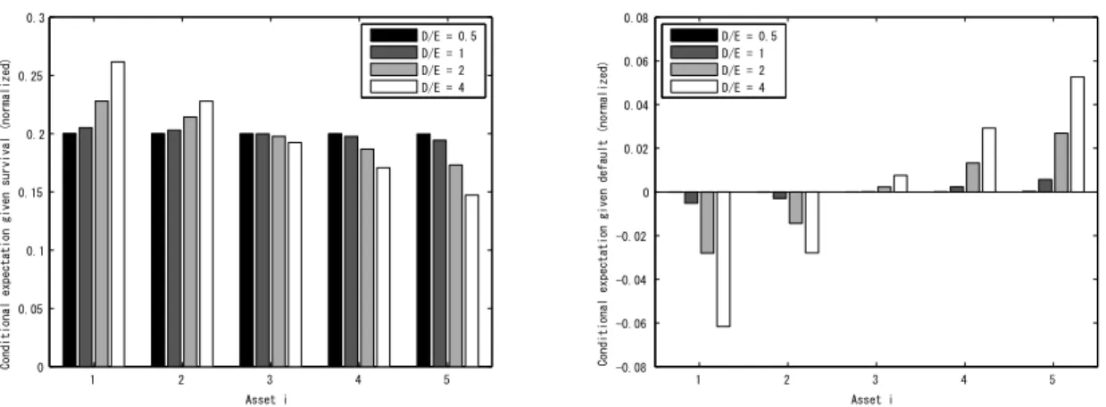
Fig. 5.1 shows the relation between the asset number vs. normalized conditional expectations given survival or default for European options. The value of each bin in the left hand side denotes the normalized conditional expectationVi(s)given survival (i.e.,AT >0) for D/E = 0.5,1,2,4 with respect to the asset numberi= 1, . . . ,5.
Since the sum of each bin with the same D/E is 1, the vertical axis may be interpreted to provide a contribution rate of assetito the equity value of the firm conditioned on survival. From the figure, we see that each equity value is indifferent on average for D/E = 0.5 in which default probability is very small, whereas the larger the volatility the higher contribution to the equity value and the difference becomes more significant with the larger D/E. This indicates that, in the case where the firm is still survival under default risk, the source of excess profit is mainly brought from a high volatility asset (or project) and the contribution of low volatility asset (or project) is not so significant. The right hand side of Fig 5.1 shows the normalized conditional expectations,
Vi(d), i= 1, . . . ,5, given the firm is default for D/E = 0.5,1,2,4 andi= 1, . . . ,5. Note thatV
(d)
i for each asset
1 2 3 4 5 0
0.05 0.1 0.15 0.2 0.25 0.3
Conditional expectation given survival (normalized)
Asset i
D/E = 0.5 D/E = 1 D/E = 2 D/E = 4
1 2 3 4 5
-0.08 -0.06 -0.04 -0.02 0 0.02 0.04 0.06 0.08
Conditional expectation given default (normalized)
Asset i D/E = 0.5
D/E = 1 D/E = 2 D/E = 4
Fig. 5.1: Normalized conditional expectations given survival (Left; V(si), i = 1, . . . ,5) or default (Right; V(i)
d , i= 1, . . . ,5) for European options
1 2 3 4 5
0 0.05 0.1 0.15 0.2 0.25 0.3
Conditional expectation given survival (normalized)
Asset i
D/E = 0.5 D/E = 1 D/E = 2 D/E = 4
1 2 3 4 5
-0.08 -0.06 -0.04 -0.02 0 0.02 0.04 0.06 0.08
Conditional expectation given default (normalized)
Asset i D/E = 0.5
D/E = 1 D/E = 2 D/E = 4
Fig. 5.2: Normalized conditional expectations given survival (Left; Vi(s), i = 1, . . . ,5) or default (Right;
Fig. 5.2 shows normalized conditional expectations for Barrier options, where the left and right hand plots compareVi(s)given survival andV
(d)
i given default, respectively, for D/E = 0.5,1,2,4 andi= 1, . . . ,5. Although
the default probability for Barrier options in Table 5.2 is much higher than that for European options for every D/E, one can observe a similar tendency for the normalized conditional expectations given survival as shown in the left hand side of Fig. 5.2, i.e., the conditional expectations given survival depends on D/E and a higher contribution to the excess profit is observed when volatility is higher. On the other hand, for the conditional expectations given default, the difference is a little emphasized compared to those for European options, in particular for D/E = 4, and the higher the volatility the higher impact on the default.
6
Conclusion
In this paper, we first generalized the optimal hedging technique with additive models in Yamada (2010–2012) for the case of path-dependent barrier options, where the problem is to find optimal payoff functions on individual options to replicate the payoff of path-dependent basket option as close as possible. To solve the necessary and sufficient condition for the optimal hedging problem, we proposed to represent the underlying assets based on the Brownian bride decomposition and showed that computations involving conditional expectations of basket barrier options may be reduced to those of unconditional expectations. We also provided an algorithm to compute the unconditional expectations using a Monte Carlo method. We then applied our methodology to the Black-Cox type first passage time structural model, where a dafaultable company is assumed to possess/run multiple assets/projects and the default may occur the first time the asset value hits a certain lower threshold before the maturity. We formulated the equity value separation problem using additive models and introduced individual equity values so that their sum approximates the total equity value as close as possible. It was also shown that any portion of total equity value may be assigned as an initial value of each individual equity when using the optimal smooth functions. Numerical experiments were also included to illustrate our methodology, in which we estimated contributions of individual equity values to default or survival by applying a certain normalization for conditional expectations.
References
[1] F. Black and J.C. Cox (1976), Valuing corporate securities: some effects of bond indenture provisions, Journal of Finance,31, pp. 351–367.
[2] F. Black and M. Scholes (1973), “The Pricing of Options and Corporate Liabilities,” Journal of Political Economy,81, pp. 637–654.
[3] P. Carr, K. Ellis and V. Gupta (1998), “Static Hedging of Exotic Options,” Journal of Finance,53(3), pp. 1165–1190.
[4] P. Carr and D. Madan (2001), “Optimal positioning in derivative securities,” Journal of Financial Econo-metrics,1(3), pp. 327–364.
[5] T. Hastie and R. Tibshirani (1990),Generalized Additive Models, Chapman & Hall.
[7] R. Merton (1973), “Theory of rational option pricing,” Bell Journal of Economics and Management Science, 4, pp. 141–184.
[8] R. Merton (1974), “On the Pricing of Corporate Debt: The Risk Structure of Interest Rates,” Journal of Finance,29, pp. 449–70.
[9] J.A. Primbs (2009), “Dynamic hedging of basket options under proportional transaction costs using receding horizon control,” International Journal of Control,82(10), pp. 1841–1855.
[10] S.E. Shreve (2004),Stochastic Calculus for Finance II: Continuous-Time Models, Springer.
[11] X. Su (2008), “Essays on Basket Options Hedging and Irreversible Investment Valuation,” Ph.D. Disserta-tion, University of Bonn.
[12] Y. Yamada (2010), “Optimal Hedging with Additive Models,” RECENT ADVANCES IN FINANCIAL ENGINEERING: Proceedings of the KIER-TMU International Workshop on Financial Engineering, World Scientific, pp. 225–245.
[13] Y. Yamada (2011), “Optimal Hedging for Multivariate Derivatives Based on Additive Models,” Proceedings of the 2011 American Control Conference, pp. 3856–3861.