つくばリポジトリ AFM 250 251 330

D

o w

i ndbr eaks r educ e t he w

at er c ons um

pt i on of

a c r op f i el d?

著者

SU

G

I TA M

i c hi aki

j our nal or

publ i c at i on t i t l e

Agr i c ul t ur al and For es t M

et eor ol ogy

vol um

e

250- 251

page r ange

330- 342

year

2018- 03- 15

権利

( C) 2017 El s evi er B. V.

U

RL

ht t p: / / hdl . handl e. net / 2241/ 00151170

Do windbreaks reduce the water consumption of a crop field?

Michiaki Sugita

Faculty of Life and Environmental Sciences, University of Tsukuba

Correspondence to: Michiaki Sugita, Faculty of Life and Environmental Sciences, University of Tsukuba, Tsukuba, Ibaraki 305-8572, Japan. E-mail:

Abstract

Two ratios,









0 0

0 0

* *

( )

( )

c a _{c avc}

u u u u

c

c avc u u c a

u u

q q _{r r}

A

r r

q q

 

 

 

 _  _{  }

 _{  }

  _  _{  }

 

 

for the canopy layer and

equivalent ratio Ag for the soil layer, were proposed for use to assess if soil evaporation

(Eg) and canopy transpiration (Ec) decrease when wind speeds are reduced by

windbreaks by a fraction of α, with qa being the specific humidity of the air, qc* the

saturated specific humidity of the canopy layer, rc the canopy resistance, and ravc the

aerodynamic resistance for moisture transfer. These ratios can be organized to form

criteria, ∆Ec < 0 (Ac < 1) and ∆Eg < 0 (Ag < 1). Thus ∆E < 0 if Ac < 1 and Ag < 1. If

only one of the ratios is smaller than unity, the sign of ∆E depends on that of ∆Eg + ∆Ec.

The criteria were examined by a dual-source crop community model to simulate energy

and water balances of a crop field with data obtained in the Nile Delta. It was found

that both ∆E ≥ 0 and ∆E < 0 were possible and ∆E was mainly determined by Eg

during the fallow and early stages of the cropping seasons and by Ec in the late

cropping period. Overall, the scale of the roughness elements hc and soil moisture θ

were found to be the major factors to determineEc, Eg, and E. A larger hc tends

Keywords dual-source crop community model; maize; Nile Delta; evapotranspiration;

1 Introduction

Effects of introducing windbreaks (WBs) on crop fields are one of the subjects

that have drawn much interest in agricultural meteorology as well as in other disciplines

(see, e.g., van Eimern et al. (1964) and Rosenberg (1979) for a review of earlier studies,

and Cleugh (1998), Steven (1998), Cleugh (2002), Brandle et al. (2004) and Helfer et al.

(2009) for a review on more recent works). This was because WBs have been

expected to produce positive effects in a wide range of practical applications in

agronomy. Evapotranspiration reduction has been one of them.

In spite of the long history of the WBs studies, however, we do not appear to

have a full understanding of evapotranspiration differences caused by an introduction of

WBs. For example, a review of Brandle et al. (2004) states that “Evaporation from bare

soil is reduced in shelter… Evaporation from leaf surface is also reduced…” as if there

is no exception. Campi et al. (2009, 2012) appear to be in this position. McNaughton

(1988) and Cleugh (1998, 2002), on the other hand, mentioned that both decrease and

increase of evapotranspiration were possible (see below in Section 2.3 for more details).

In reality, there have been studies that reported increase (e.g., Baker et al., 1989),

decrease (e.g., Miller et al, 1973; Campi et al., 2009, 2012), and both decrease and

contradiction is perhaps not surprising because the influence of WBs on crop fields is

quite complex.

McNaughton (1983) argued one such complexity of WBs that there are both

direct and indirect effects on evapotranspiration of WBs. The direct effects arise from

an altered turbulent exchange between the surface and the atmosphere. The indirect

effects represent changes in evapotranspiration due to modified crop characteristics

developed in different microclimates caused by WBs. Field studies based on

measurements in a crop field with WBs often observe the combined effects of the direct

and indirect effects. Theoretical approaches often focus on part(s) of such effects.

Thus the purposes of our study were (i) to revisit this problem of whether or not,

evapotranspiration should decrease by the introduction of WBs; and (ii) to clarify major

factors that cause the evapotranspiration differences due to WBs. In order to achieve

these goals, first, we summarize available theories to study WBs influences, followed

by the Methods section which introduces dual-source and single-source crop

community models and dataset to be used in numerical experiments to simulate and

compare energy and water balance with and without WBs. Finally, the Results and

Discussion section list and discuss our findings. We focus our study on the direct

crop community. However, to facilitate comparison with previous studies, results from

the single-source model are also presented. Also, in our experiments, the microclimate

including temperature, humidity, and wind speeds in the internal boundary layer above

the vegetated surface in the leeward of WBs is assumed given.

2 Theory

2.1 Influence of wind speeds reduction on a crop community

To study the influence of WBs, it was first assumed that a crop community

consists of two layers, the canopy layer and the soil layer. Surface latent heat fluxes are

expressed by the following bulk transfer equations (see, e.g., Brutsaert, 1982; Garratt,

1992)









*

( )

*

( )

e c a

e c

c avc

p c a

c avc L q q L E =

r r c e e

r r 

 

   



(1)









*

( )

*

( )

e g a

e g

g avg

p g a

g avg

L q q

L E =

r r

c e e

r r

 



   



(2)

for the soil layer. Le is the latent heat of vaporization;  is the atmospheric density; cp

is the specific heat of air at constant pressure; γ is the psychrometric constant; ea and qa

are respectively the vapor pressure and specific humidity both in the air; and e* and q*

are the saturated value of vapor pressure and specific humidity at single-source surface

temperature. In Eqs. (1) – (2), and in the rest of this study, the subscript g and c

represent the soil layer and canopy layer, respectively, and those without a subscript

indicates the whole community. Thus Eg is the soil evaporation; Ec is the canopy

transpiration; and E is the crop community evapotranspiration. rc is the canopy

resistance; rg is the soil resistance; and ravc and ravg are the aerodynamic resistance for

scalar transfer. Similarly, the sensible heat fluxes Hc and Hg are formulated by the

following bulk equations (e.g., Brutsaert, 1982; Garratt, 1992)





c p hc c a

H = c C u T T (3)





g p hg g a

where Ch is the bulk transfer coefficient for sensible heat which is assumed to be the

same as Ce, an equivalent coefficient for water vapor. Tais the air temperature, T is the

single-source surface temperature, and u is the wind speed.

When wind speed is reduced above each layer, the following reaction should

take place according to Eqs. (1) and (2):

1

( )

c avc

c avc c

E

u r

r r H

 

 

     _{    }

    _{    }

  (5)

and

1

.

( )

g avg

s avg g

E

u r

r r H

 

 

         

    _{    }

   

(6)

An up or downward arrow beside each variable(s) indicates an increase or a

decrease of the variable(s), respectively. From the 1st to the 2nd term of Eqs. (5) and (6),

turbulence is weakened as shown by the increase of ravcand ravg, which should then

reduce the turbulent exchanges of Ec, Hc, Eg, and Hg (3rd and 4th terms). However, the

decrease of the outgoing fluxes (4th term) would induce an increase of source

concentration, i.e., the single-source surface temperature Tcand Tg, as well as saturated







*



*

4

c a _c

c a c

c c

c c _c

c nc

c

T T _E

q q H

E T

H q _E

T R H      _{ }  _{   }          __ _ _ _    _  _             _{   }   _{  }      _{ }     (7) and







*



* 4

g a g

g g a

g g

g g _g

g ng

g

T T E

H

q q

E T

H q _E

T R H         _{  }          _  _ _ _      _{ }              _{   }           _{ }  _{ }  (8)

where Rn is the net radiation;



is the Stefan-Boltzmann constant; T is in K. From the

3rd term of Eqs. (7) and (8), there are two separate paths, one indicating increases of the

gradients leading to the fluxes increases (negative feedback), and another showing a

decrease of the net radiation, and the resulting decrease of H and E fluxes (positive

feedback). Because there are feedback loops, an equilibrium should be reached (at

least temporarily) for a given condition, somewhere in Eqs. (5) and (7), and Eqs. (6) and

(8). The key variables that determine the equilibrium position are Tc and Tg because

they link the bulk equations Eqs. (1) – (4) with energy balance equations of the crop

community (see A.1.1. in the Appendix). Thus the equilibrium must be reached at the

2.2 Criteria to determine the fate of evapotranspiration

In view of Eqs. (1) and (2), it is convenient to define the ratio Ac

















0

0 _{0 0}

0 0 0 0 * * * * ( ) ( ) ( ) ( )

cu u c a c a

c

c avc c avc

c u u _{u u u u}

c a _{c avc}

u u u u

c avc u u c a

u u

E q q q q

A

r r r r

E

q q _{r r}

r r q q       _{ }            _  _{  }  _{  }   _  _{  }     (9)

and the ratio Ag

















0

0 0 0

0 0 0 0 * * * * ( ) ( ) ( ) ( )

g _{u u g a g a}

g

s avg s avg

g u u u u u u

g a _{u u} g avg _{u u}

g avg

g a _{u u}

u u

E _{q q q q}

A

r r r r

E

q q r r

r r q q                    _{    }  _{  }   _{    }       (10)

to argue the fate of Eg, Ec, and E when u becomes weaker from uu₀ to uu₀

( 0  1 ). As is clear, whether WBs should reduce evapotranspiration can be judged by comparing the magnitude of the change in the gradient of the q concentration and

that in resistances for the humidity transport. When the gradient change is larger (Ac > 1

or Ag > 1), the equilibrium is reached in the 2nd – 4th term in the upper path of Eqs. (7) –

< 1 or Ag < 1), the equilibrium is likely reached in Eqs. (5) – (6) and Ec and Eg should

decrease. Thus Ac and Ag can be organized to formulate the following criteria,













0 1

0 1 ,

0 1 c c c c A E A A        _  _ _{ }    (11)













0 1 0 1 0 1 g g g g A E A A         _  _         (12) and





































































































































1 1

0 1 1

1 1

1 1

0 1 1

1 1

1 1

0 1 1

1 1

c g

c g c g

c g c g

c g

c g c g

c g c g

c g

c g c g

c g c g

A A

A A E E

A A E E

A A

E A A E E

A A E E

A A

A A E E

A A E E

  _{   }     _  _{       }        _        _   _{     }  _{ }  _{ }   _{ }        _     _        _  _{   }       _        _                                           _ (13)

in which symbols and represent the logical operation of “and” and “or” respectively.

In our study, the Δx symbol represents the difference between x for α = 1.0 and x for a

2.3 Analysis based on the Penman-Monteith equation

It is also possible to study E in a simpler manner if one assumes a single-source model. McNaughton (1988) and Cleugh (1998, 2002) have introduced this

approach by using the Penman-Monteith (P-M) equation given by











_ _



* 1

1 /

n p a a

PM

e c PM a PM

s R G c e e

E

L s r r

 

 _{  } 

  

 

 

  (14)

where EPM is the evapotranspiration; Rn is the net radiation; G the soil heat flux; s is the

slope of the saturation vapor pressure (ea*) curve at Ta; ra_PM is the aerodynamic

resistance; and rc_PM is the surface resistance.

Whether evapotranspiration would be reduced when wind speed u was decreased

can be studied by evaluating the sign of E_PM /u. It is convenient for this purpose to replace ra_PM with

2

0 0 0 0

0 0

1 /

ln ln

e av

v m

v

k

C u r

z d z d z d z d

z L z L

 

  _{ }      _{ }   

   

 _{ }  _{ }

   

(15)

where z is the measurement height of u, Ta, and ea; d0 is the zero-plane displacement

stability correction function with the subscript v and m representing vapor and

momentum transport (e.g., Brutsaert, 2005); and L is the Obukhov length. With a

simple manipulation, it is possible to show













_ _ _ 0 0 0

c c eq PM

c c eq c c eq

r r E r r u r r       _{ }             (16)

where rc_eq is the equilibrium canopy resistance defined by





_ * a a c eq eq q q r E    (17)

in which Eeq is the equilibrium evaporation.





1

eq n

e

s

E R G

L s 

 

 . (18)

As can be understood by referring to Eq. (17), rc_eq is the canopy resistance that would

be necessary to produce E =Eeq under the actual dryness of the air (qa* − qa).

Note that McNaughton (1988) and Cleugh (1998) used different expressions

from Eqs. (16) – (17). McNaughton (1988)’s version is













* * *

0 ( )

0 ( )

0 ( )

a a eq

PM

a a eq

a a eq

q q D

E

q q D

u

q q D

and Cleugh (1998)’s version reads,













0

0

0

PM eq PM PM

eq eq PM

E E

E

E E

u

E E

  

 

 _{ } 

 

  

 

 

 

(20)

in which D_eq E r_{eq c PM_} /. It is easy to show that Eqs. (16) - (17) can be converted into Eq. (19) or Eq. (20).

In our study, we mainly focus on the framework given in sections 2.1 – 2.2;

however, to facilitate a comparison with previous studies, Eq. (16) will also be

examined.

3 Methods

3.1 Dual-source crop community model

A dual-source crop community model was used to understand how soil

evaporation Eg and transpiration Ec would respond to reduced wind speeds by means of

WBs under given soil, vegetation, and meteorological conditions. The model consists

of the canopy layer and the soil layer, and energy and water balance of the two layers

The details of the model are explained in the Appendix. Briefly, those processes

above the soil surface were formulated by means of three energy balance equations for

the canopy layer, for the soil layer, and for the crop community; it was assumed that

interactions between the atmosphere and the canopy layer, and those between the

atmosphere and the soil surface work side by side, and the sum of the two fluxes results

in the community level flux to satisfy the conservation equations (Kondo and Watanabe,

1992). Subsurface hydrological processes from the surface down to water table were

also included in the model. They were formulated based on previous proposals with

locally calibrated parameters whenever possible. Soil moisture content θ was then

derived as the residual of the soil water balance equations and used to estimate the soil

resistance r_avgand the canopy resistance r_avc which control Eg and Ec, respectively.

3.2 Dataset

A dataset obtained in an irrigated crop field without WBs in the Nile Delta in

Egypt was used as inputs to the model. The details of the site, measurements, and

experiments are explained in El-Kilani and Sugita (2017) and Sugita et al. (2017);

in the central part of the Delta. An eddy correlation system together with

meteorological and hydrological instruments was mounted on and around a 5-m tower

at the center of a 200 by 200 m crop field (see Table 3 of Sugita et al. (2017) for the

details of the measurements). In our analysis, those data obtained in the summer of

2011 were mainly used. The 2011 summer season consists of a fallow season (May 21

– June 13) and a summer cropping season (June 14 – September 17) in which maize

(Zea mays L., cv., Three Ways Cross (Hybrid) 324) was cultivated using the furrow

irrigation method with an irrigation interval of approximately two weeks. Other

relevant variables of vegetation, soil, irrigation, etc. were also measured in this field.

3.3 Numerical experiments

3.3.1 Experiment I

In this experiment, nine sets of simulated outputs of energy and water balance

components for a hypothetical crop field were generated for the 2011 summer season

under various assumed conditions. El-Kilani and Sugita (2017) also produced six

similar sets. In each set, simulations were carried out with wind speeds u specified as a

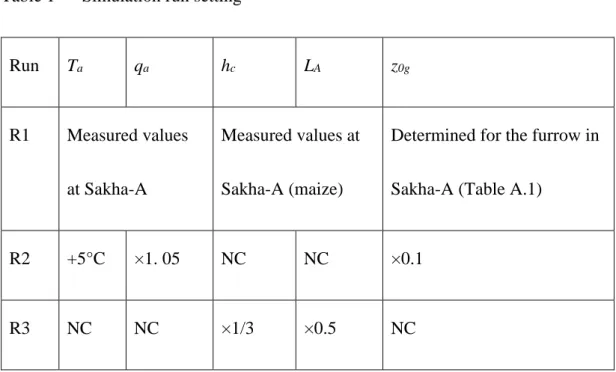
study, three sets of outputs (run R1 – R3; Table 1), each with =0.1, 0.9 and 1.0, were

chosen out of these 15 sets so that the selected cases represent a wide variety of

conditions and results of Ec, Eg, and E.

Run R1 is the baseline case representing the maize field without WBs with the

measured meteorological variables used as inputs. Run R2 represents the case in which

Ta, qa, and the soil surface roughness z0g were altered from those of run R2. We varied

z0g to represent the surface condition of a different irrigation method. The z0g value for

the furrow irrigation is generally larger than that for a flat soil surface using drip and

basin irrigation. By varying qa, the case of altered microclimate in the so-called quiet

and wake regions in the leeward of WBs can be realized. The magnitude of the qa

variation was determined from the observed differences between qa in the leeward and

in the windward of WBs in a field experiment in the Nile Delta (El-Kilani and Sugita,

2017). In the same experiment, the Ta differences were found negligible; nevertheless,

we varied Ta in run R2 to see the influence of a different climatic condition.

The setting of run R3 is the same as that of run R1 except for the size of the

crop, and the crop height (hc) and leaf area index LAI (LA) were altered from those of

zone depth zrz, and the canopy cover fraction fcc, while the change of hcalters

momentum and scalar roughness lengths (see Appendix).

3.3.2 Experiment II

This experiment was intended to focus specifically on the influence of the scale

of roughness elements on ΔE, ΔEc, and ΔEg under the same condition as run R1 of

experiment I. However, the simulations were carried out only for one day, August 1,

selected arbitrarily from the midseason stage of maize. This was because

meteorological conditions do not affect much in the outcome of ΔE, ΔEc, and ΔEg (see

also the results presented in section 3.3) and that increased soil moisture to saturation

did not produce markedly different simulated results for August 1, as was found in a

preliminary analysis.

The same model was used except that the soil water balance part was disabled

and water content value on this day determined in run R1 was prescribed as an input.

The canopy height hc was varied from the actual value of 2.2 m in the range of 0.1 < hc

on Aug.1) was adopted regardless of hc in this experiment. The difference between the

result for = 0.1 and those for 1.0 was examined.

4 Results and discussion

4.1 Different responses of the canopy and soil layers

Fig. 1a and b indicate the relation between ΔE and E_c for the two cases of α = 0.1 and 0.9 based on the outputs of the experiment I. Clearly, both E > 0 and E < 0 occurred, which agree with McNaughton (1988) and Cleugh (1998, 2002), and

assessments of observational studies mentioned in the Introduction section. It was

found that E > 0 accounts for approximately 50 - 60%. A general positive correlation (R2 = 0.83 - 0.85) can be noticed between E_c and ΔE, if we ignore the points with E_c= 0 during the fallow season and other outlier points among the results of run R2 (α = 0.1) during the crop development stage when LA and hc were still small

and soil surfaces were not fully covered by vegetation.

g

E

 < 0 constitutes 32% while that of E_c< 0 and E_g> 0 accounts for 21%. In the case of α = 0.1, the percentages are 36% and 8%, respectively.

These results tend to imply that a single-source treatment of a crop community is

likely an oversimplification if we need to study all stages of the cropping season. On

the other hand, if the only target is the stages with mature canopy, it is likely acceptable

to work with a single-source model.

Fig. 1e and f show whether the criterion given by Eq. (16) produced predictions

of ΔE which agree with the ΔE results of the simulation runs. For this purpose, the

outputs of runs R1, R2 and R3 of experiment I were organized accordingly and shown

in Fig.1e for α=0.1, and in Fig.1f for α=0.9. The value of rc_PM was determined by

inverting Eq. (14) with the simulated values of E, Rn, G, and by setting ra_PM = rav in Eq.

(17). It is immediately clear that there are cases which do not agree with what Eq. (16)

suggests in both figures.

There should be at least four possible causes which induced failure of the

criterion Eq. (16) to predict ΔE. First is the case when the sins of ΔEc and ΔEg were

different. Failure is possible in this case because the canopy and the soil layers are

open triangles or green squares symbols based on Eqs. (9) and (10). The majority of

those points against Eq. (16) are found for r_{c PM_} /r_{c eq_} 1 and  E 0, but some are for

_ / _ 1

c PM c eq

r r  and  E 0. The second cause is related to the fact that Eq. (16) is based on the derivative of the P-M equation evaluated at uu₀ to estimate the change in E for an infinitely small change of u while E was determined for a finite difference of uu₀ and uu₀; naturally they are not necessarily the same. The third cause originates from the fact that (16) does not consider the change in Rn resulting from the

single-source surface temperature changes as indicated by Eqs. (7) and (8). Finally, the

assumption in the derivation of the P-M equation,

* *

* _{s a}

a s a

e e de

s

dT T T



 

 , could be the

source of disagreement. It is this assumption that allows us to use



e_a*e_a



, instead of the specific humidity difference between evaporating surface and the atmosphere



qs qa



, as one of the driving forces of evapotranspiration.

4.2 Factors that influence E_c, E_g, and E

Since surface fluxes are closely linked to the turbulent exchange between the

candidate to investigate as the main factor to determine E_c, E_g, and E. This was studied with the results of experiment II (Fig. 2a – c).

Fig. 2a indicates that









0

0 * 0.1 * c a u u c a u u q q q q   

 > 1 and

0

0

( )

( )

c avc u u c avc _{u u} r r r r    

 > 1 for all hc

values. This was caused by the increase of *

c

q and r_avcas u decreased and the turbulent

exchange was suppressed (Eq. (5)). Rnc always decreased as u decreased (Eq. (7)).

It can also be noticed that 0

0

0.1

( )

( )

c avc u u c avc _{u u} r r

r r







 decreased while









0

0 * 0.1 * c a u u c a u u q q q q    

increased when hc increased. As a result, Ac kept increasing and became larger than 1.0

at hc=1.93 m. This is where E_c started to take positive values. Thus Ec tends to

decrease when u is reduced for a smaller canopy while Ec increases are more likely to

occur for a larger canopy. This is qualitatively in agreement with the assessment of

Cleugh (1998) who showed, based on the P-M equation, the increase of the possibility

of E reduction as the aerodynamic resistance increased (that is, as hc decreased).

The fact that 0

0

0.1

( )

( )

c avc u u c avc _{u u} r r

r r







 decreased as hc increased means that (rcravc) is

more sensitive to the u change when the scale of the roughness elements is smaller.

This can be understood by evaluating









 

2

1 / 1 /

c avc h h

r r C u C u

u u

 _{ }  _{ }

  for a

hc = 0.2 m, d0 = 2/3hc, and zov = 6.8 10-3),



r_c r_avc



u  _

 = − 42 at u=2 m/s (z = 10 m/s).

For a large canopy, Ch = 0.006 (z0 = 0.15 m, hc = 2 m, d0 = 2/3hc, and zov= 2.0 10-2 m),

and



r_c r_avc



u

 _

 = −63 for the same wind speed. Therefore,

0

0

0.1

( )

( )

c avc u u c avc _{u u} r r

r r







 is 50%

larger for the small canopy.

The same observations can be made for the soil layer (Fig. 2b) except that Ag < 1

and E_g< 0 all the time and their dependence on hc is weak. As a result, the relation

between E and hc is similar to that between E_cand hc except that E< 0 for all hc

values examined. Overall, it can be concluded that the size difference of the roughness

elements affects mainly E_c, and to a lesser degree E_g.

3.3 Seasonal changes in E_c, E_g, and E

In order to investigate how other factors than the roughness scale influence

evapotranspiration differences due to WBs, a comparison was made between the

Fig. 3a and b clearly show the same dependence of E_c, E_g, and Eon the roughness size observed in Fig. 2a - c: the canopy part is more sensitive to the

roughness scale than the soil surface part; and 0

0

0.1

( )

( )

c avc u u c avc u u

r r

r r



 

 decreased,









0

0 * 0.1 * c a u u c a u u q q q q   

 increased, and Ac increased as hc increased, particularly at later stages

of the cropping season (after the middle of July). In this periods, ΔEc≫ΔEg and thus

ΔEc essentially controls the fate of ΔE. ΔEc (and thus ΔE) shows a general decrease as

hc increased. However, these changes are not monotonous, unlike the case of Fig. 2a -

c. For example, 0

0

0.1

( )

( )

c avc u u c avc u u

r r

r r



 

 shows periodic peaks in response to irrigation events.

The same behavior can also be observed for









0

0 * 0.1 * c a u u c a u u q q q q   

 . Those changes were

caused by the increases in the θ value and resulting decreases in rc and rg. This agrees

with Cleugh (1998) in general who indicated that wet soil conditions tended to result in

the reduction of E. Also noticed in the figures are that the impact of irrigation was more

pronounced in the early stages of the cropping season. This is because the root zone

became deeper at later stages (Sugita et al., 2017) and therefore the soil moisture

In addition, it can be noted that in the fallow and early cropping seasons

(through the middle of July), ΔE = ΔEg or ΔE≒ΔEg and thus behavior of ΔEg is

important. ΔEg is mostly positive and shows periodic negative values. The cases of

ΔEg < 0 correspond to the periods of increased θwith irrigation events. This is why

ΔEg > 0 most of the time during the fallow season with small θ without irrigation

events.

Seasonal changes in meteorological elements such as incoming radiation, air

temperature, humidity and wind speed did not significantly affect E_c, E_g, and E. This is partly because the climate in Egypt is stable (Sugita et al., 2017) and seasonal

fluctuations in these elements were small during the cropping season. Therefore this

part of the results could be area specific. Indeed, a comparison of the simulated results

of different Ta and/or qa values (results not shown) has indicated that the increased Ta

and qa tend to enhance the magnitude of E_c and E_g for α < 1 while the increase of

qa alone weakened E_c and E_g.

Overall, factors which affected the seasonal changes in E_c and E_g can be summarized as the height of the roughness elements and surface resistance mainly

5. Conclusions

In order to study the influence of windbreaks on crop evapotranspiration, two

ratios (Eqs. (9) and (10)) have been proposed using the framework of a dual-source crop

community model. They were organized to form the criteria given by Eqs. (11) - (13)

to determine whether windbreaks could reduce evapotranspiration (ΔE < 0).

It was shown that both ΔE > 0 and ΔE < 0 occurred in the results of the

numerical experiments under three different conditions with two cases of wind speeds

reduction by a fraction of α = 0.1 and 0.9 using the dataset obtained in a crop field in the

Nile Delta. The results with ΔE > 0 account for approximately 50 - 60%. Generally,

∆E > 0 can be observed as canopy height increased. This was because the main factor

that determines ∆Ec and ∆Eg is the turbulent exchange which is influenced by the

roughness scale. An additional contribution was made by the soil moisture increase

due to irrigation events which reduce surface resistance for humidity transport above the

soil and canopy layer. As a result, ∆Ec and ∆Eg decreased with θ increases.

speeds were found to have a minor influence in the case of the dataset obtained in the

Nile Delta.

The results with different signs of ΔEc and ΔEg account for 42% (α = 0.1) and

53% (α = 0.9). In these cases, the sign of ΔE was determined mostly by ΔEg during the

fallow and early cropping seasons and by ΔEc as the canopy height increased. The

correlation between ΔEc and ΔEg was very weak. ΔEc and ΔE, on the other hand, show

a higher correlation in the later stages of cropping season with mature canopy. As a

result, a single-source treatment of a crop community is not recommended to study

windbreaks influences, particularly in the early stages of the cropping season when the

soil surface plays an important role in the surface-atmosphere interaction; this can be

treated better by the dual- or multi-layer crop community models. Indeed, the criterion

(16) proposed based on the Penman-Monteith (P-M) equation did not always produce

correct predictions of ΔE.

Acknowledgements

Authors are also grateful for El-Kilani, Rushdi M.M. (Cairo University) for

University) and Hoshino, A. (Univ. Tsukuba) for providing us with their soil moisture

and soil physics data, for Kubota, A. and Maruyama, S. (Univ. Tsukuba) for sharing

their results on plant physiology and observation, for Fukuda, T., Matsuno A., Shimizu,

T., Tsuchihira, K., Irigaki, Y. and Tsuji, I. (Univ. Tsukuba) for their participation in the

field observations, and for Osada, A., Kamitani, T., Sayed El Nehlak, Hassan Mohamed

Abd El Baki, and Hussein Al Nadar, among others (WAT project office, JICA) for

supporting field observations for this study. Finally, the authors also express their

appreciation to Satoh, M. (Univ. Tsukuba) without whose initiatives and leadership the

experiment for this study would not have been possible. This research has been

supported and financed, in part, through SATREPS of JST/JICA.

Appendix

A.1 Dual-source crop community model

A.1.1 Energy balance

The energy balance equation can be expressed as,





4 4

(1 ) (1 ) 2(1 )

nc c sd su ld c g c c c e c

R   f R R R   f T   f T H L E (A.1)





4 4

(1 )

ng c sd su ld c c g g e g

R  f R R R   f T T H L E G (A.2)

for the soil layer, and as





4 4

(1 )

n sd su ld c g c c g e g c e c

R  R R R _fT   f T _H L E H L E G (A.3) for the crop community. In Eqs. (A.1) – (A.3), Rsd and Rsu are the downward and

upward short-wave radiation; Rld is the downward long-wave radiation; fc is the canopy

transmissivity; and G is the soil heat flux.

A.1.1.1 Resistance parameterizations

The soil resistance rg was estimated by

1

1

1.75 0

( )

273.16

b s g

g a r

T D

 



 

 

 

(A.4)

(Kondo et al., 1990) where D0 = 2.23×10-5 m2/s is the molecular diffusivity at soil

surface temperature Tg = 0°C, and a1 and b1 are the soil-type specific constants. Model

calibration with the data during the fallow period allowed determination of these

The canopy resistance rc was estimated based on the so-called Jarvis-type

models (e.g., Jacquemin and Noilhan, 1990),

 





   



*



,min/ 1 2 3 4

c st A sd a a a

r r L f R f e e f T f  (A.5)

where rst,min is the minimum bulk stomatal resistance, f1 through f4 (0 f 1 ) are

respectively a function of Rsd, that of (ea* – ea), and so on. The same functional forms

of Jacquemin and Noihen (1990) were adopted, but the coefficients were determined by

the resistance measurements of maize in the Sakha-A field (Kubota, 2014, personal

comm.). They are,

,min 1 ,max 1 1 st st r f F r F   _  _{ }

  (A.6)

where rst, max is the maximum bulk stomatal resistance and F is another function

1 0.55 sd gl A R F R L    _ _

  (A.7)

and













2









* 2

* *

2

0.1 10 hPa

1 10 hPa

a a

b

a a a a

e e f

a e e e e

 _{ }       _  _    (A.8)

The value of rst, min was also adopted initially from the in situ measurements by Kubota

(2014, personal comm.), but in the calibration stage, it was adjusted to produce the best

cropping season of maize, after the parameters of rg had been calibrated (see section

A.3). The final value together with coefficients a2 and b2 are listed in Table A.1. Other

functions are





2

3 1 3 a ref, a

f  a T T (A.9)

where a3 = 0.0016 (Jacquemin and Noihan, 1990) is a coefficient, and Ta,ref is the air

temperature that produces the smallest rst, and

4

w fc w f  

 



 . (A.10)

in which θw is θ at the wilting point and θfc is the field capacity.

The values of rac and rag were determined from Eq. (15) and the equivalent

equation for the soil layer from bulk transfer coefficients (see below in section A.1.1.2).

A.1.1.2 Bulk transfer coefficients

The bulk transfer coefficients of the maize community for sensible heat Ch were

determined from Eq. (15) for each time step with momentum roughness z0and scalar

roughness z0h by assuming similarity between the sensible heat and latent heat transport.

z0hg. Finally, the bulk transfer coefficients for the canopy layer Chc were determined

from

hc h hg

C C C . (A.11)

The momentum roughness of the soil surface z0gwas determined by applying

the method of Toda and Sugita (2003) in which the z0g value was selected, that

produced the best agreement of friction velocity u* values estimated from the profile

equation in the surface layer,

0 0

*

0

( ) ln m

z d z d

u u z

k z L

      

 _{  }  _{ }

 

 

  (A.12)

and those measured by the eddy correlation method(Sugita et al., 2017). The

application was made to the data during the fallow season when d0=0 and z0=z0g. The

selected z0g value (Table A.1) is larger than the textbook value for bare soil surfaces.

This is reasonable as the Sakha-A field was cultivated using furrow irrigation (the bed

interval: 0.8 m, and the bed width and height: 0.2 m each). The larger z0g obviously

reflects this rougher surface condition.

The scalar roughness length of the soil surface z0hg was also determined by the

same procedure. However, instead of u* values, the sensible heat fluxes H were

0 0

* 0

( ) ln

g a h

p h

z d z d

H

T T z

kuc z L

      

  _{  }  _{ }

 

 

  (A.13)

and in the analysis, d0 = 0 and z0h = z0hg were assigned.

Also determined were the momentum roughness z0 and the scalar roughness for

sensible heat z0h of the crop community. The determination was made several times

during the maize cropping season by applying the same procedure outlined above. The

following regression equations were derived that relate canopy height hc with z0 and z0h

2 3

=0.0292 + 0.000828 0.00573 + 0.0135

0 c c c

z h  h h (A.14)



2



=exp 6.76 0.284 0.677

0h c c

z   h  h

from which daily values were estimated.

A.1.1.3 Wind speeds below canopy

For the application of Eqs. (2) and (4), the wind speeds below canopy at z = zg

were estimated from the measured wind speeds above the canopy. zg = 0.1 m was

arbitrarily selected. First, ( )u h_c was estimated from the measurement at z = 5.78 m by

applying the wind profile equation Eq. (A.12). Then the wind profile function below





4

( _g) ( ) exp_c 1 _g / _c

u z u h _a z h _ (A.15)

was applied to ( )u h_c for the case of hc > 0.1 m, with the coefficient a4 = 2.0 based on

Inoue and Uchijima (1979). The estimated u z( _g) was finally converted to u at z = 5.78

m by applying (A.12) for use in the model. When hc  0.1 m, the measured u at z =

5.78 m was simply used in the model by ignoring the small canopy.

Note that wind profile functions such as (A.15) have been developed from the

horizontal equation of motion in the absence of a pressure gradient and the Coriolis

force but with a momentum sink term due to the presence of stems and leaves below a

canopy. Assumptions were then made that the shear stress is proportional to the wind

speed gradients by means of eddy viscosity Km and that the sink term is proportional to

u(z), the foliage drag coefficient cdf and the foliage surface area Af. (A.15) can be

obtained if we assume of a constant value of Afcdf and a constant mixing length (and

thus Km). Other functions can be obtained by assuming a different form of Km (e.g.,

Cowan, 1968). Also, adopting different closure scheme other than the mixing length

approach allows derivation of different forms (e.g., Yi, 2008); however, this approach is

not without criticism (Finnigan et al, 2015). Massman et al. (2017) adopted a

parameterization of u*/u(hc) as a function of height and proposed a wind profile model

profile and another near the surface. It was aimed to represent a realistic wind profile

near the surface, which should be close to a logarithmic shape with u(z) approaching

zero at z0.

Although it was tempting to use the model by Massman et al. (2017) as it likely

produces a more realistic value of u z( _g)near the surface, it was decided not to adopt

this model at present since it was tested only by one profile measurement for maize. In

contrast, (A.15) has been tested and used extensively and successfully in the literature.

However, to test uncertainties to use (A.15), u z( _g)values from (A.15) were changed by

±15% in the numerical experiments, and the results were compared against those from

simulations without change of u z( _g). The conclusions obtained in our study with

(A.15) were found to remain the same with ±15% changes of u z( _g)values.

A.1.1.4 Canopy transmittance and coverage

The canopy transmittance fc and LAI (LA) were determined by a canopy analyzer

(Li-cor, LAI2200 or LAI2000) several times during the maize cropping season at

made around noon for the fc measurement, and shortly after sunset for LA. These data

were used to determine the following empirical equation





1 1.015 1 exp 0.633

c A

f   _   L _ (A.16)

which was used to estimate the daily value of fc as a function of LA in the model.

The canopy cover fraction fcc was necessary to estimate infiltration of rainfall

differently under the canopy and in the canopy gaps. However, no rainfall was recorded

during the 2011 summer season, and fcc was therefore not used for our study.

Nevertheless, for the sake of completeness, the empirical function adopted in the model

is given below as

0.551

34.097

cc A

f  L . (A.17)

in which its functional form and coefficients were determined by comparing the

measured LAand fcc values. The values of fcc were determined by image processing of

digital camera images taken at a nadir-looking position at eight locations in the field

(Tsuchihira, 2011; see also Byambakhuu et al, 2010 for the details of the method).

The water balance equations for the crop community including the soil layer

beneath the surface are given by

w s

g rz rz c

dS dS

I W I E

dt   dt     (A.18)

s

i r g g

dS

P P I E

dt     (A.19)

in which Pi is the irrigation, Pr is the rainfall, Ss is the surface water storage resulting

from Pi or Pr, Ig is the infiltration into the soil at soil surface, Irz is the drainage from the

bottom of the root zone z = zrz, Wrz is the upward capillary flux evaluated at zrz, and Sw is

the water storage in the form of soil moisture in the soil layer. Also, the community

level evapotranspiration is given by

g c

EE E . (A.20)

The thickness of the soil layer was arbitrarily determined as 0.17 m for the fallow

season and set equal to the depth of the root zone (zrz) during the cropping season which

was given as a function of LA (see below in section A.1.2.3).

Soil water content was estimated as a residual of Eq. (A.18) – (A.19) by

considering two cases. The first case was when the top of the capillary fringe on water

table was within the soil layer. In this case, saturation was simply assumed in the soil

layer. Then, the mean θ in the soil layer was estimated in the model by solving soil

water balance Eq. (A.18) for Sw. To determine which case applies, the depth to water

table (zgw) was used. The depth of the capillary rise was assumed constant at air entry

value (Hb) (see Table A.1).

A.1.2.1 Depth to water table

Groundwater level was measured continuously in an observation well of a depth

of 2 m. The timing and amount of the irrigation were also recorded (Sugita et al.,

2017). They were used to derive the relation between zgw and the elapsed time t (d)

measured from the end of the last irrigation event. It was found that the relationships

observed in different events looked similar, and therefore it was decided to estimate zgw

in meters by the following empirical function fitted to the measurements,











5



1.1 1 exp 0.115 / 2

gw

z  _   t _

 . (A.21)

A.1.2.2 Soil water balance components

In Eq. (A.19), Pr can be neglected for the present purpose to apply the model in

an i-th time step was determined from S i( )S i(  1) _P i_i(  1) I i_g(  1)_ t in which

Δt is the time step employed for the model implementation (=1 d). The infiltration into

the soil at surface Ig was estimated from the following expression of Milly (1986),

1 0.5 5

5 2

0

4

1 1 1 gc

g

a i

I a

A



 _{   } 

 _{ } 

 _    _{  }

   

 _{ } 

 

(A.22)

which makes use of the infiltration capacity (Philip, 1957). In Eq. (A.22), a5 is a constant

and assumed as 1/2 of the hydraulic conductivity Ks (Table A.1); A0 is the sorptivity and

was estimated from

1/ 2 0

0.165 0.67

0 1.458 u s

A   K d



 

 _



_ (A.23)

(Eq. (11) of Milly (1986)), in which  is the matric head, and _uis at satiation with

 =0 (Table A.1). The values of A0 for different depth ranges of the root zone were

calculated by Eq. (A.23) and are listed in Table A.1). igc is the cumulative infiltration

(Philip, 1957) given by

1/ 2

0 5

gc

i A a (A.24)

in which τ is the elapsed time measured from the start of the irrigation event.

Parameters in these equations (Table A.1) were derived from soil samples taken in the

Sakha-A field and subsequent laboratory experiments (Fujimaki and Hoshino, 2010,

The drainage Irz from the bottom of the root zone z = zrz was determined by

( )

rz rz

I K  (A.25)

in which K( ) is the unsaturated hydraulic conductivity as a function of soil water

content θ at zrz. The K( ) values of soil samples taken in the Sakha-A field were

determined by Fujimaki and Hoshino (2010, Personal comm.). The parameter a6 (Table

S.1) of the following expression by Brooks and Corey (1966) was determined by fitting

Eq. (A.26) to the data,

6 6

( 2 3 )/

( )

a a s

s

K  K 



  

 _{ }

  . (A.26)

The upward capillary flux Wrz was set equal to zero because soil water potential

measurements at two levels (−0.7 and −0.9 m) above water table indicated steady

downward moisture flux (Fujimaki, personal comm., 2013).

A.1.2.3 Root zone depth

The depth of the root zone was determined from root distribution measurements

of Tsuchihira (2011), and additionally from the data of Fujimaki (2014, personal

of 0.2×0.2×0.1 m taken from the surface to −0.5 m at a 0.1-m interval. For our study,

the following functional relationships were established for the maximum depth zrz

obtained for maize using the drip irrigation and using the furrow irrigation.









0.483exp / 1.092 0.49 (furrow)

0.550 exp / 0.352 0.56 (drip)

A rz

A L z

L

 



  _{ }

 . (A.27)

In the case of zrz < 0.1 m, zrz = 0.17 m was arbitrarily assigned.

A.2 Model implementation

The simulation was carried out starting on April 1 in experiment I, to provide a

spin-up period for the model to produce reasonable soil moisture at the beginning of the

summer season on May 21.

The model was solved for each time step by employing an iteration procedure.

More specifically, initial guess values of Tg and Tc were assigned and this allowed initial

estimations of Hg, Eg, Hc, and Ec from Eqs. (1) - (4), which were then inserted into the

right-hand side of Eqs. (A.1) – (A.3) and Eqs. (A.18) – (A.19) to examine whether or

not the energy balance of each layer closed sufficiently. If the closure was not

balance closure; this process was repeated until the closure had been achieved

sufficiently (<5 W/m2) for both (A.1) and (A.2).

The model was operated at a daily time step. The atmospheric stability was

considered. This was because evapotranspiration takes place mainly during daytime

under unstable atmospheric conditions, and even if daily averaging was employed,

resulting daily mean fluxes of H, E and u* usually indicate unstable conditions.

Therefore the daily values of the Obukhov length L were determined from the measured

daily mean values of H, LeE and u* and were used in all simulation runs. Note that a

more accurate treatment should have been an iteration procedure, in which the first H

and LeE values produced by the model, and u* obtainable from the wind speed data and

the profile equation Eq. (A.12) with assumed neutral stability, can be used to derive the

first estimate of L, which in turn allows the second estimate of the fluxes, and so on.

However, this is quite complicated and was not adopted because the stability correction

functions s are only a mild function of z/L.

A preliminary analysis carried out to compare the results from hourly simulation

and those from daily simulation did not show significant differences so that the

A.3 Model calibration

The estimated values of E and Eg were compared with the measurements in

order to calibrate the coefficients in Eqs (A.4) and (A.5). As mentioned above, it was

aimed to produce the best agreement between the measured E and the simulated E

values, on average. A regression constant a = 1.00, the coefficient of determination R2

= 0.94 for a regression equation through the origin yax (x and y represent the simulated and the measured variables), and the RMS difference = 0.51 mm (defined as





₂ 0.5

/ i i

x y n

 _ 





 ) were obtained for the fallow season; similarly, a = 0.99, R2 = 0.97,

and the RMS difference = 0.70 mm were obtained for the cropping season. On average,

the model reproduced E values (or Eg during the fallow season) reasonably well (see

also Fig. A.1.

A comparison was also made visually between the measured and the simulated

time series variables of E, θ, and Rlu, the upward long wave radiation (Fig. A.2).

Although the time changes in all three variables are well reproduced by the model, the

agreement in terms of magnitude is not necessarily excellent, particularly for θ.

not propagate into the evapotranspiration estimation too much. This was partly because

References

Baker, G.L., Hatfield, J.L., Wanjura, D.F., 1989. Influence of wind on cotton growth

and yield. Trans. ASAE, 32, 97-104.

Brandle, J.R., Hodges, L., Zhou, X.H., 2004. Windbreaks in North American

agricultural systems. Agrofor. Syst., 61, 65-78.

Brooks, R.H., Corey, A.T., 1966. Properties of porous media affecting fluid flow.

Proc. Am. Soc. Civ. Eng., J. Irrigation Drainage Div. IR2, 61-68.

Brown, K.W., Rosenberg, N.J., 1972. Shelter-effects on microclimate, growth and

water use by irrigated sugar beets in the great plains. Agr. Meteorol., 9, 241-263.

Brutsaert, W., 1982. Evaporation into the Atmosphere: Theory, History, and

Applications. D. Reidel Pub. Co., Dordrecht.

Brutsaert, W., 2005. Hydrology: An Introduction. Cambridge University Press,

Cambridge.

Byambakhuu, I., Sugita, M., Matsushima, D., 2010. Spectral unmixing model to assess

land cover fractions in Mongolian steppe regions. Remote Sens. Environ., 114,

Campi, P., Palumbo, A.D., Mastrorilli, M., 2009. Effects of tree windbreak on

microclimate and what productivity in a Mediterranean environment, Eur. J. Agron.,

30, 220-227. doi:10.1016/j.eja.2008.10.004

Campi, P., Palumbo, A.D., Mastrorilli, M., 2012. Evapotranspiration estimation of crops

protected by windbreak in a Mediterranean region. Agri. Wat. Manage, 104,153–162,

doi:10.1016/j.agwat.2011.12.010

Cleugh, H.A., 1998. Effects of windbreaks on airflow, microclimates and crop yields.

Agroforestry Systems, 41, 55-84.

Cleugh H.A., 2002. Parameterising the impact of shelter on crop microclimates and

evaporation fluxes. Australian J. Exp. Agricul., 42, 859-874.

Cowan, I.R., 1968. Mass, heat and momentum exchange between stands of plants and

their atmospheric environment. Q. J. R. Meteorol. Soc. 94, 523-544, doi: 

10.1002/qj.49709440208

El-Kilani, R.M.M. and Sugita, M., 2017. Irrigation methods and water requirements in

the Nile Delta. In: M. Satoh and S. Aboulroos, eds. Irrigated Agriculture in Egypt-