Control of stabilization parameter in bubble function FEM based on the SUPG method
( Application to micro channel flow problems )
Shigetosshi Tai*
Graduate School of Nagaoka University of Technology 1603-1 Kamitomioka, Nagaoka, Niigata, Japan
Email: [email protected]
Takahiko Kurahashi Nagaoka University of Technology 1603-1 Kamitomioka, Nagaoka, Niigata, Japan
Email:[email protected]
Summary
We discuss the stabilization parameter in the bubble function FEM based on the SUPG method. The FEM using the stabilized bubble function element is applied to analyze the rotating cone and the two phase flow problems. In addition, the CSF model is included in numerical simulation of two phase flow problem. In this study, the rotating cone problem is carried out to investigate the numerical of the accuracy of the bubble function FEM using the stabilization parameter in the SUPG method. In addition, the numerical simulation of the two phase flow is carried out based on the FEM using the present bubble function element.
Keywords: Microchannel, FEM, Bubble function, SUPG method, Liquid-Liquid Two-Phase Flow
1 Introduction
Figure 1: Micro-chemical chip
In recent years, various technology developments are carried out using a micro chemical chip (see Figure 1).
For instance, there is a study on the solvent extraction [1].
When the solvent extraction is conducted, it is necessary to make a parallel two phase flow in a micro scale space.
The governing equations, i.e., the Navier-Stokes, the continuity, and the advection equations, are used to represent the two phase flow field. In addition, the surface tension of the fluid in the micro-scale flow channel is represented by the CFS model [2]. As the discretization method, the bubble function FEM using the stabilization parameter in the SUPG method is applied. Furthermore,
the θ method is employed for discretization in time.
In this study, the rotating cone problem is carried out to investigate the advantages of bubble function FEM using stabilization parameter in the SUPG method. Based on the result, we carried out the numerical simulation of the two phase flow in measurement area. In addition, results between numerical simulation and experiment are compared.
2 Governing equation
In this study, the Navier-Stokes equations shown in Equation (1) and (2) are applied to compute flow field.
V ˙ i +V j V i, j + 1
ρ P
,i− ν (V i, j +V j,i )
,j = f i (1)
V i,i = 0 (2)
where V i , P, ρ , ν , and f i V indicate the velocity components, the pressure, the density, the viscosity coefficient and the body force per unit volume. In two phase flow, the interface position is given by the solution of the advection equation shown in equation (3).
φ ˙ +V i φ
,i= 0 (3)
Two kind of fluids are separated by value of index
function φ . The fluid properties ρ , ν are expressed by those
of two fluid ρ
(n), ν
(n)(n=1, 2) and the index function φ such as ρ = (1 − φ ) ρ
(1)+ φρ
(2), ν = (1 − φ ) ν
(1)+ φν
(2). Here, in case of φ = 0 and φ = 1, fluid properties ρ and ν indicate ( ρ
(1), ν
(1)) and ( ρ
(2), ν
(2)), respectively. In addition, the CSF model [2] is applied to express the interfacial tension force. Interface or surface tension is given by Equation (4).
f i V = σκ ρ
,iρ ˆ ρ
ρ ˜ (4)
where σ and κ indicate interface or surface tension coefficient and curvature, and curvature κ is expressed as Equation (5).
κ = | 1 n n n |
[ n i
| n n n | | n n n |
,i− n i,i ]
(5) where n i indicates direction cosine, and is given by the gradient of index function φ
,i.
3 Interpolation function
As the interpolation function of the flow velocities and the index function, the bubble function elements is applied (see Figure 2). In addition, the linear triangular elements is applied to interpolate the pressure (see Figure 3). Interpolation function for flow velocities, pressure and index function are written as Equations (6), (7) and (8).
Figure 2:
Bubble function element
Figure 3:
Linear triangular element
V i = N
1V i1 + N
2V i2 + N
3V i3 +N
4V ˜ i4 = { N B }
T{ V i } (6) P = N
1P
1+ N
2P
2+ N
3P
3= { N }
T{ P } (7) φ = N
1φ
1+ N
2φ
2+N
3φ
3+ N
4φ ˜
4= { N B }
T{ φ } (8) where, N
1, N
2, N
3and N
4indicate shape function, and the shape function is expressed by area coordinate ( η
1, η
2, η
3).
N
1= η
1, N
2= η
2, N
3= η
3, N
4= 27 η
1η
2η
3(9) V ˜ i4 and ˜ φ
4are expressed by Equations (10) and (11).
V ˜ i4 = V
4− 1
3 (V
1+V
2+V
3) (10) φ ˜
4= φ
4− 1
3 ( φ
1+ φ
2+ φ
3) (11)
4 Discretization of the transport equation
In this section, the discretization of the transport equation that represents the movement of the fluid interface is carried out. The transport equation shown in Equation (3) is represented as Equation (12) by the θ method.
φ n+1 + ∆t(1 − θ )V i n+1 φ
,in+1 = φ n −∆t θ V i n φ
,in (12) where θ is a parameter varied in the range of 0 ≤ θ ≤ 1.
Moreover, the weighted residual equation can be expressed as Equation (13). The weighting function of the index function φ is given by w
φ.
∫
Ωew
φφ n+1 dΩ + ∆t(1 − θ ) V ¯ i n+1
∫
Ωew
φφ
,in+1 dΩ
=
∫
Ωew
φφ n dΩ −∆t θ V ¯ i n
∫
Ωew
φφ
,in d Ω (13) The weighting function w
φis interpolated by bubble function element such as the index function as shown in Equation (14).
w
φ= N
1w
φ1+N
2w
φ2+ N
3w
φ3+ N
4w
φ4= { N B }
T{ w
φ} (14) Considering Equations (8) and (14), Equation (13) can be written as Equation (15).
∫
Ωe{ N B }{ N B }
TdΩ{ φ n+1 } +∆t(1 − θ ) V ¯ i n+1 ∫
Ωe
{ N B }{ N B,i }
TdΩ{ φ n+1 }
=
∫
Ωe{ N B }{ N B }
TdΩ{ φ n }
−∆t θ V ¯ i n
∫
Ωe{ N B }{ N B,i }
TdΩ{ φ n } (15) Therefore, the finite element equation is represented by Equation (16).
[M] { φ n+1 } +∆t(1 − θ ) V ¯ i n+1 [G i ] { φ n+1 }
= [M] { φ n } − ∆t θ V ¯ i n [G i ] { φ n } (16) Each integral term in Equation (16) is denoted by Equations (17) and (18).
[M] =
∫
Ωe{ N B }{ N B }
TdΩ (17)
[G i ] =
∫
Ωe{ N B }{ N B,i }
TdΩ (18)
5 The stabilization control parameters in the bubble function element
The stabilization parameter τ Bubble Mom. for bubble function element shown in Equation (19) has been proposed [3], and this parameter is derived such that stabilization parameter in the SUPG method shown in Equation (20) is equivalent to that in the FEM using bubble function element.
τ Bubble Mom. =
( ∫
Ωe
N
4d Ω )
2( ν + ν
′) ∫
ΩeN
4,iN
4,id Ω A e (19)
τ SU PG = (( 2
∆t )
2+ ( 2 | U |
h )
2+ ( 4 ν
h
2)
2)
−12(20) where ν
′and indicates numerical viscosity parameter and area of element, and the stabilization parameter is only operated at bubble function point, gravity point, in element, i.e., in the finite element equation for the motion equation, the numerical viscosity shown in Equation (21) is added at the bubble function point.
( ν + ν
′) ∫
Ωe
N
4,iN
4,idΩ
=Ae1
(
∫ΩeN
4dΩ )
2(
(
∆t2)
2+ (2|U|h
)2
+ (4ν
h2
)2)1
2
(21)
where | U | and h indicate magnitude of velocity in each element and mean element length, and h is given by √
2A e . In addition, the interpolation function for index function is written as Equation (8).
In the finite element equation for the advection equation, the numerical viscosity shown in Equation (22) is added at the bubble function point.
ν
′∫
Ωe
N
4,iN
4,idΩ
= 1 A e
( ∫
Ωe
N
4d Ω )
2((
2
∆t )
2+ ( 2 | U |
h ))
12(22) 6 Rotating cone problem
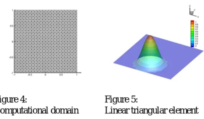
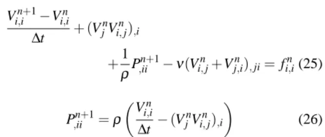
In this section, the rotating cone problem is carried out to investigate the advantages of the bubble function FEM using stabilization parameter in SUPG method. The spatial distribution of variable φ represented in the equation (23) (see Figure 5) is given as shown in Figure 4. The advection velocity field given by the u = − y and v = x. The bubble function element without the stabilization parameter is employed in case 1, the bubble function element with the stabilization parameter which is equivalent to that by the SUPG method is employed in case 2.
φ =
{ 0.5(cos(2 π r) + 1) r ≤ 0.5
0 r > 0.5 (23)
Figure 4:
Computational domain
Figure 5:
Linear triangular element Computational conditions are shown in Table 1. In addition, computational results are shown in Table 2. It is found that the numerical damping can be controlled by using the bubble function element with the stabilization parameter.
Table 1: Computational conditions Number of nodes 1,681 Number of elements 3,200 Time increments 0.001 Time step 6,280
Table 2: Comparison of cone height in cases 1 and 2
Round Coordinates Cone height in case 1 in case 2 0
φ(x=0.0,y=-0.5)
1.0000000 1.0000000
1 0.9566303 1.0010651
2 0.9083724 0.9980166
3 0.8254727 0.9935277
4 0.7544963 0.9928489
7 Flow simulation in the micro-channel
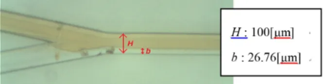
In this section, based on the results of the rotating cone problem, the numerical simulation of the two phase flow in measurement area shown in Figure 6 is carried out. Discretization of the governing equation are indicated below.
7.1 Discretization and derivation of pressure Poisson equation
The discretization of the pressure Poisson equation is carried out to obtain the solution of the pressure field.
The Navier-Stokes equation shown in Equation (1) is represented as Equation (24) by the Euler method.
V i n+1 − V i n
∆t +V j n V i, n j + 1
ρ P
,in+1 − ν (V i, n j +V j,i n )
,j = f i n (24)
where ∆ t is a time increment. Equation (25) can be derived
by differentiating the Equation (24). Moreover, the pressure
Poisson equation can be expressed as Equation (26).
V i,i n+1 − V i,i n
∆t + (V j n V i,j n )
,i+ 1
ρ P
,iin+1 − ν (V i, n j +V j,i n )
,ji = f i,i n (25)
P
,iin+1 = ρ ( V i,i n
∆t − (V j n V i, n j )
,i)
(26) Based on Equation (26), the finite element equation of the pressure Poisson equation shown as Equation (27) is derived by Galerkin method.
[C ii ] { P n+1 }
= − ρ ¯ ( 1
∆t [S i ] { V i n } + V ¯ j n [D i j ] { V i n } )
+ { B n } (27) Each integral term in Equation (27) is denoted by the following Equations (28) - (31).
[C ii ] =
∫
Ωe{ N
,i}{ N
,i}
TdΩ (28) [S i ] =
∫
Ωe{ N }{ N B,i }
TdΩ (29) [D i j ] =
∫
Ωe{ N
,i}{ N B, j }
TdΩ (30)
{ B n } = ρ ¯ V ¯ j n ∫
Γe{ N }{ N B, j }
T{ V i n } n i dΓ +
∫
Γe{ N }{ N
,i}
T{ P n+1 } n i dΓ (31) 7.2 Discretization of the Navier-Stokes equations
The discretization of the Navier-Stokes equation is carried out to obtain the solution of the equation of motion.
The discretized equation in time is expressed as Equation (32).
V i n+1 = V i n − ∆ t (
V j n V i, n j + 1
ρ P
,in+1 − ν (V i, n j +V j,i n )
,j − f i n )
(32) Finally, the finite element equation of the Navier-Stokes equation shown as Equation (33) is derived by Galerkin method.
[M] { V i n+1 }
= [M] { V i n } − ∆t (
[A(V j n )] { V i n } − 1
ρ ¯ [S i ]
T{ P n+1 } + ν
(
[H j j ] { V i n } + [H ji ] { V j n } )
− { F i n } + { T i n } )
(33)
Each integral term in Equation (33) is denoted by the following Equations (34) - (38). { F i n } and { T i n } represent the external force and the traction force terms.
[M] =
∫
Ωe{ N B }{ N B }
Td Ω (34) [A(V j n )] =
∫
Ωe{ N B } ( { N B }
T{ V j n } ) { N B, j }
TdΩ (35) [S i ]
T=
∫
Ωe{ N B,i }{ N }
TdΩ (36) [H j j ] =
∫
Ωe{ N B, j }{ N B, j }
Td Ω (37) [H ji ] =
∫
Ωe{ N B, j }{ N B,i }
TdΩ (38) 7.3 Computational condition
The computational conditions of numerical simulation are shown in Table 3. Two finite element analysis mesh for two phase flow in micro channel are shown in Figure 6. Ethyl acetate Q
(1)and pure water Q
(2)are injected from left side of the channel. Water quantity of ethyl acetate is 10[ µ l/min], and that of pure water is 50[ µ l/min].
Table 3: Computational conditions
Total number of nodes 11,991 Total number of elements 23,200 Time increment∆t (sec.) 3×10⁻⁷
Time steps 1,400,000
Densityρ(1)(kg/mm3) 9.982×10⁻⁷ Kinematic eddy viscosityν(1)(mm3/sec) 0.557
Densityρ(2)(kg/mm3) 8.984×10⁻⁷ Kinematic eddy viscosityν(2)(mm3/sec) 1.004