New Local Search Methods for Improving the Lagrangian Relaxation-Based Unit Commitment Solution

New Local Search Methods for Improving

the Lagrangian Relaxation-Based Unit Commitment Solution

Guidance

Associate Professor Nobuo YAMASHITA

Takeshi SEKI

2006 Graduate Course in

Department of Applied Mathematics and Physics Graduate School of Informatics

Kyoto University

KYOTO UNIVER SITY FO

U N^KYOTODED 1^JAPAN897

February 2008

Abstract

The unit commitment problem (UCP) for an electric power system is to determine the schedules of power units that minimize the total production cost over a planning horizon while satisfying the load demand, spinning reserve, and operating constraints of individual units. The UCP is formulated as a nonlinear mixed-integer programming problem that includes 0-1 variables representing the on-off states of the units. When the number of units is large and the planning horizon is long, the UCP is a large-scale problem, for which an exact optimal solution is difficult to obtain within a reasonable computation time. Therefore, several methods have been proposed to obtain an approximate solution of the UCP. Among these methods, the Lagrangian relaxation (LR) method is useful for large-scale UCPs. The LR method is first used to solve the dual problem of the UCP and is then used to construct a feasible solution from the dual solution by using some heuristics. However, the quality of the feasible solution is not satisfactory.

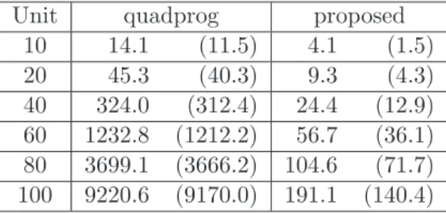
In the present paper, we propose new local search methods for improving the feasible solution obtained by the LR method. We define the neighborhood of the local search as the feasible set in which the schedules of all but one or two units are fixed. The neighborhood search can then be executed by solving the one-unit or two-unit commitment problems, which are efficiently solved by dynamic programming. In this search, quadratic programming problems with a particular structure should be solved frequently. Since a general quadratic programming solver does not exploit such a special structure, a great deal of time is required when the number of units is large. Therefore, we also propose a technique for solving the quadratic programming problems efficiently by exploiting the particular structure of the quadratic programming problems.

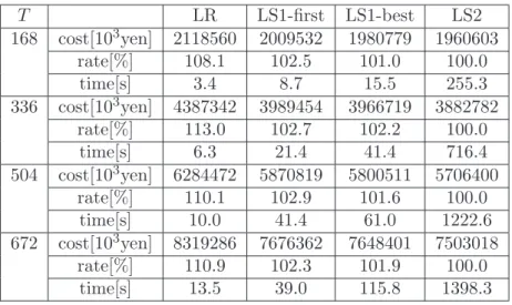
Numerical results show that the proposed local search methods can find feasible schedules for

which the costs are lower than those obtained by the existing methods, which are based on mixed-

integer programming or genetic algorithms. The applicability of the proposed methods to long-term

UCPs is also demonstrated.

Contents

1 Introduction 1

2 Unit Commitment Problem 2

2.1 Notation . . . . 2

2.2 Formulation . . . . 2

3 Lagrangian Relaxation Method 4 3.1 Maximization of the Dual Problem . . . . 6

3.1.1 Subgradient Method for the Dual Problem . . . . 6

3.1.2 Dynamic Programming for the Lagrangian Relaxed Problem . . . . 6

3.2 Construction of a Feasible Solution . . . . 9

3.2.1 Finding a Reserve-Feasible Schedule . . . . 9

3.2.2 Economic Dispatch . . . . 11

4 New Local Search Methods for the Unit Commitment Problem 12 4.1 One-unit Local Search . . . . 13

4.2 Two-unit Local Search . . . . 15

5 Numerical Results 17 5.1 Comparisons of the Quadratic Programming Solvers for ED(t) and (4.1) . . . . 17

5.2 Comparisons with the Existing Methods for the Benchmark Problems . . . . 18

5.3 Behavior of the Proposed Methods for Long-term Problems . . . . 20

6 Conclusion and Future Research 20 A Approximate Methods for the Calculation of Costs in Local Search 23 A.1 An Approximate Method for the Calculation of g _{˜ i} (t; u _{˜ it} ) . . . . 23

A.2 An Approximate Method for the Calculation of g _{˜ i ˜ j} (t; u _{˜ it} , u _{˜ jt} ) . . . . 25

B Problem Data for the Numerical Experiments 28

1 Introduction

Electric power is an essential form of energy in modern life. In many countries and in certain areas, thermal power generation is a major source of power and reducing the production costs is important.

The price of electricity is linked with production costs, especially fuel costs. In recent years, steep increases in the price of natural resources such as heavy oil or natural gas have increased the production costs of thermal power plants.

Power generation systems usually consist of several thermal units. The unit commitment problem (UCP) is to determine the schedules and generations that minimize the total production cost over the planning horizon while satisfying the load demand, spinning reserve, and operating constraints of individual units. The UCP is commonly formulated as a nonlinear mixed-integer programming problem with 0-1 variables representing the on-off states of the thermal units. As such, when the number of units is large and the planning horizon is long, the problem is an extremely large-scale problem. The exact optimal solution of such a large-scale UCP is difficult to obtain in a practical computation time.

Several methods have been proposed by which to obtain an approximate solution of the UCP efficiently [13], including priority list methods [14], dynamic programming (DP) [15], branch-and- bound methods (B&B) [9], mixed-integer programming (MIP) [7], and Lagrangian relaxation methods (LR) [2, 11, 12, 8]. The priority list method is the simplest of these methods and is able to obtain a feasible solution within a short computation time, even if the problem size is large. However, the obtained solution is not satisfactory. Although methods such as DP, B&B, and MIP can theoretically obtain an exact (or near exact) solution, they require an impractical computation time for a large- scale UCP. The LR method basically solves the dual problem of the UCP. The objective function of the dual problem is represented as the optimal value of the Lagrangian relaxed problem, which can be decomposed into small subproblems of each unit. Using this characteristic, we can obtain the dual solution of the UCP efficiently even if the problem size is large. However, in general, obtaining the solution through dual optimization is not feasible for the UCP. Therefore, we must find a feasible solution by some heuristics. The main disadvantage of the LR method is that such a feasible solution is often unsatisfactory.

In the present paper, we consider the large-scale UCP, which consists of several units over a long planning horizon. Therefore, we apply the LR-based method. As stated above, the LR-based feasible solution is often disappointing. In order to overcome this disadvantage, we propose new local search methods to improve the feasible solution. Methods to improve the LR-based solution have been proposed in previous studies [16, 12]. However, since the method proposed in [16] uses mixed-integer programming, it is not suitable for large-scale UCPs. In the method proposed in [12], a local search method is proposed in the present study. This method represents the continuous operating states as one block in order to satisfy the minimum up time constraints and replaces the blocks to improve the solution. Since the local search is restricted to individual blocks, the improvement is limited.

We therefore propose new local search methods, in which we may modify the schedules of one or

two units freely. Therefore, the proposed methods can achieve a wider search than the method of

[12]. Therefore, we expect that the methods proposed herein can obtain a better solution. However,

expanding the search area of the local search might cause a long computation time. In the present

paper, we also propose a technique based on the nonlinear optimization for efficient neighborhood search of the proposed local search methods.

The remainder of the present paper is organized as follows. Section 2 describes the formulation of the common unit commitment problem considered herein. The Lagrangian relaxation procedure for the UCP is discussed in Section 3. Section 4 presents a detailed description of the proposed local search methods. Numerical results are presented and discussed in Section 5. Finally, conclusions are presented in Section 6.

2 Unit Commitment Problem

In this section, we formulate the unit commitment problem (UCP).

2.1 Notation

The following notation will be used herein.

Indices:

i Index for unit.

t Index for time period.

Constants:

I Set of units.

T Total number of time periods.

S _i ^hot Hot startup cost of unit i.

S _i ^cold Cold startup cost of unit i.

D _t Load demand in time period t.

R _t Spinning reserve in time period t.

p ^max _i Maximum generation of unit i.

p ^min _i Minimum generation of unit i.

∆ _i Maximum ramp-rate of unit i.

t ^up _i Minimum uptime of unit i.

t ^down _i Minimum downtime of unit i.

t ^cold _i Cold startup time of unit i.

Decision Variables:

p _it Generation of unit i in time period t.

u _it 0-1 state variable of unit i in time period t (u _it = 1: on, u _it = 0: off).

v _it Number of time periods in which unit i has been on or off during time period t (v _it > 0: unit has been on, v _it < 0: unit has been off).

We denote the vectors (u _i1 , . . . , u _iT )

and (p _i1 , . . . , p _iT )

as u

and p

, respectively. Moreover, u and p denote the schedules and generations of all units. Throughout the reminder of the present paper, one time period corresponds to one hour.

2.2 Formulation

The objective function of the UCP represents the total production cost over the planning horizon.

The total production cost consists of the fuel cost and the startup cost.

The fuel cost of unit i in time period t is usually given as the following convex quadratic function of p _it :

f _i (p _it ) = a _i p ² _it + b _i p _it + c _i , (2.1) where coefficients a _i , b _i , and c _i are generally nonnegative.

The startup cost is related to the energy necessary to turn on a unit that has been off and occurs only when the unit is turned on during time period t (u _i,t−1 = 0 and u _it = 1). In general, the startup cost depends on the number of the time periods that the unit has been off. In the present paper, we assume that two types of startup costs, S _i ^hot and S _i ^cold , are given. Here, S ^hot _i represents the ”hot startup cost”, which is required when a hot off-unit is turned on (when the number −v _it of time periods the unit has been off is below t ^down _i + t ^cold _i ). On the other hand, S _i ^cold represents the ”cold startup cost”, which is required when the cold off-unit is turned on (when the number of −v _it of time periods the unit has been off is greater than t ^down _i + t ^cold _i ). The startup cost of unit i in time period t is then given as

S _i (v _i,t−1 , u _it , u _i,t−1 ) =

( u _it (1 − u _i,t−1 )S _i ^hot if v _i,t−1 < −t ^down _i − t ^cold _i

u _it (1 − u _i,t−1 )S _i ^cold if v _i,t−1 ≥ −t ^down _i − t ^cold _i . (2.2) Using (2.1) and (2.2), the objective function φ of the UCP is defined as

φ(p, u) = X T

t=1

X

i∈I

{u _it f _i (p _it ) + S _i (v _i,t−1 , u _it , u _i,t−1 )}. (2.3)

The constraints of the UCP consist of the system constraints and operating constraints of indi- vidual units.

System Constraints

• Demand constraints:

D _t = X

i∈I

u _it p _it , t = 1, . . . , T. (2.4)

• Spinning reserve constraints:

R _t ≤ X

i∈I

u _it (p ^max _i − p _it ), t = 1, . . . , T. (2.5) The spinning reserve constraint is used in the case of an unexpected increase in the demand or a unit failure. Using (2.4), (2.5) is rewritten as

D _t + R _t ≤ X

i∈I

u _it p ^max _i , t = 1, . . . , T. (2.6)

Operating Constraints of Thermal Unit

• Generation limit constraints:

u _it p ^min _i ≤ p _it ≤ u _it p ^max _i , t = 1, . . . , T. (2.7a)

• Minimum uptime constraints:

u _it = 1 if 1 ≤ v _i,t−1 < t ^up _i , t = 1, . . . , T. (2.7b)

• Minimum downtime constraints:

u _it = 0 if − 1 ≥ v _i,t−1 > −t ^down _i , t = 1, . . . , T. (2.7c)

• State transition equations for t = 1, . . . , T : v _it =

( min(t ^up _i , max(v _i,t−1 , 0) + 1) if u _it = 1

max(−t ^down _i − t ^cold _i , min(v _i,t−1 , 0) − 1) if u _it = 0. (2.7d)

• Ramp-rate limit constraints:

|p _it − u _it p _i,t−1 | ≤ ∆ _i , t = 1, . . . , T. (2.7e)

The minimum uptime (downtime) constraints mean that a unit must be on (off) for a certain number of time periods once it has been turned on (off). The ramp-rate limit constraints mean that a generation cannot change quickly.

Consequently, the UCP is formulated as P ⁰ : min

p;u

φ(p, u)

s.t. (2.4), (2.6), (2.7).

The problem P ⁰ is a mixed-integer programming problem including 0-1 variables. Here, P ⁰ is in the class of NP-hard problems, and an exact optimal solution to this problem is difficult to obtain.

3 Lagrangian Relaxation Method

In this section, we explain the Lagrangian relaxation (LR) method for solving the UCP.

The LR method basically solves the dual problem of the UCP. First, we focus on the relationship between the primal and dual problem of the UCP. Let the dual problem of P ⁰ be denoted by D ⁰ . Then, from the duality theory [3], the following inequality holds:

min(P ⁰ ) ≥ max(D ⁰ ).

Hereinafter, we remove the ramp-rate limit constraints (2.7e) from P ⁰ for simplicity. Let P denote P ⁰ without (2.7e).

P : min

p;u

φ(p, u) s.t. D _t = X

i∈I

u _it p _it , t = 1, . . . , T D _t + R _t ≤ X

i∈I

u _it p ^max _i , t = 1, . . . , T

(p _i , u _i ) ∈ U _i , ∀i ∈ I,

where

U _i := {(p _i , u _i ) | (p _i , u _i ) satisfies (2.7a), (2.7b), (2.7c), and(2.7d)}.

Since the feasible region of P includes that of P ⁰ , the following inequality holds:

min(P ⁰ ) ≥ min(P).

Since the inequality

min(P) ≥ max(D) holds by the duality theory, we have

min(P ⁰ ) ≥ max(D).

Therefore, the optimal value of D provides the lower bound for P ⁰ as well as P. Note that if a feasible solution of P satisfies the ramp-rate limit constraints (2.7e), then it also is feasible for P ⁰ .

In the reminder of the present paper, we focus on the problem P. Now, we define the Lagrangian function L as

L(p, u, λ, µ) := φ(p, u) + X T

t=1

λ _t (D _t − X

i∈I

u _it p _it ) + X T

t=1

µ _t (D _t + R _t − X

i∈I

u _it p ^max _i ),

where λ _t ∈ <, t = 1, . . . , T and µ _t ≥ 0, t = 1, . . . , T are the Lagrangian multipliers to (2.4) and (2.6), respectively, λ = (λ ₁ , . . . , λ _T )

and µ = (µ ₁ , . . . , µ _T )

.

Using the Lagrangian function L, the dual problem of P can be written as D : max θ(λ, µ)

s.t. µ ≥ 0,

where the dual function θ(λ, µ) is defined by the optimal value of the Lagrangian relaxed problem:

min

L(p, u, λ, µ)

s.t. (p _i , u _i ) ∈ U _i , ∀i ∈ I, (3.1)

that is,

θ(λ, µ) = min

p,u

{L(p, u, λ, µ) | (p _i , u _i ) ∈ U _i , i ∈ I}.

If min(P) > max(D) holds, then the duality gap exists. In general, there exists a duality gap for the UCP. If φ(p, u) − θ(λ, µ) is small for given feasible solutions (p, u) and (λ, µ) of P and D, respectively, then (p, u) is considered to be a good approximate solution of P. Thus, we want (λ, µ) to be the maximum solution of D.

Note that even if the maximum (λ

, µ

) of D is obtained, the solution ( ˆ p, u) of the Lagrangian ˆ

relaxed problem (3.1) with (λ

, µ

) is not always feasible for P. Thus, we must find a feasible solution

of P from the solution ( ˆ p, u) of the problem (3.1). Therefore, the Lagrange relaxation method is ˆ

executed in two steps: the maximization of the dual problem (Subsection 3.1) and the construction

of a feasible solution (Subsection 3.2).

3.1 Maximization of the Dual Problem

The dual problem D is a nondifferentiable convex problem. In order to solve such a problem, the subgradient method [2] and the bundle method[6] are useful. In [6], it is reported that the bundle method requires fewer iterations to converge, as compared to the subgradient method. However, the quadratic problem must be solved in each iteration. Since the cost of solving the quadratic programming problem is much greater than that of solving the relaxed problem (3.1), the effect of the reduced number of iterations of the bundle method is limited. Therefore, in the present paper, we apply the standard subgradient method to solve the dual problem.

3.1.1 Subgradient Method for the Dual Problem

Here, we explain the subgradient method for the dual problem of the UCP. Now, let (p ^k , u ^k ) denote the solution of the Lagrangian relaxed problem (3.1) for (λ ^k , µ ^k ). Then, the subgradient ξ ^k of the dual function is given by

ξ ^k =



 

 

 

 



D ₁ − P

i∈I p ^k _i1 .. .

D _T − P

i∈I p ^k _iT D ₁ + R ₁ − P

i∈I u ^k _i1 p ^max _i .. .

D _T + R _T − P

i∈I u ^k _iT p ^max _i



 

 

 

 



∈ ∂θ(λ

, µ

). (3.2)

Using this subgradient ξ ^k , the standard subgradient method updates Lagrangian multipliers as µ λ ^k+1

µ ^k+1

¶

= max

½ 0,

µ λ ^k µ ^k

¶

+ δ _t ^k ξ ^k kξ ^k k

¾

, (3.3)

where

δ ^k = 1

² + σk , ² > 0, σ > 0. (3.4)

Note that δ ^k is the step size, and ² and σ are constant parameters.

The subgradient method for D is described as follows.

Subgradient Method for the Dual Problem D

¶ ³

Step 0: Select initial Lagrangian multipliers (λ ⁰ , µ ⁰ ). Set k := 0.

Step 1: Solve problem (3.1) for (λ ^k , µ ^k ) and obtain the solution (p ^k , u ^k ).

Step 2: If the stopping criteria is satisfied, then set ( ˆ p, u, ˆ λ, ˆ µ) := (p ˆ ^k , u ^k , λ ^k , µ ^k ) and terminate.

Otherwise, go to Step 3.

Step 3: Update (λ ^k+1 , µ ^k+1 ) by (3.3), set k := k + 1, and go to Step 1.

µ ´

3.1.2 Dynamic Programming for the Lagrangian Relaxed Problem

The main task of the subgradient method is to solve the Lagrangian relaxed problem (3.1). Next, we

explain the solution of the Lagrangian relaxed problem (3.1) by dynamic programming (DP) .

First, note that the dual function is separated as θ(λ, µ) = X

i∈I

θ _i (λ, µ) + X T

t=1

{λ _t D _t + µ _t (D _t + R _t )}, where θ _i (λ, µ) is defined by the optimal value of the following problem:

min X T

t=1

[u _it {f _i (p _it ) − λ _t p _it − µ _t p ^max _i } + S _i (v _i,t−1 , u _it , u _i,t−1 )]

s.t. (p _i , u _i ) ∈ U _i .

(3.5)

Problem (3.5) is a subproblem of unit i and can be solved efficiently by the following DP algorithm.

DP is an enumeration method based on the principle of optimality (see [4] for details on DP). The optimal solution of the problem (3.5) is obtained by enumerating the costs of all states from time period 1 to time period T . Recall that v _it denotes the state of unit i during time period t and that the number of all states during each time period is t ^down _i + t ^cold _i + t ^up _i + 1. Let C _i (t, v _i ) denote the cost when the state of unit i during time period t is v _it . Now, assume that the costs C _i (t − 1, v _i,t−1 ), v _i,t−1 = −t ^down _i − t ^cold _i − 1, . . . , −1, 1, . . . , t ^up _i during time period t − 1 are calculated. From (2.2), (2.7b), and (2.7c), the state of unit i must be one of the following:

1) Possible to turn on with cold startup cost S _i ^cold in the next time period (v _i,t−1 = −t ^down _i −t ^cold _i − 1),

2) Possible to turn on with hot startup cost S _i ^hot in the next time period (−t ^down _i ≥ v _i,t−1 ≥

−t ^down _i − t ^cold _i ),

3) Impossible to turn on in the next time period (−1 ≥ v _i,t−1 > −t ^down _i ), 4) Impossible to turn off in the next time period (1 ≤ v _i,t−1 < t ^up _i ), 5) Possible to turn off in the next time period (v _i,t−1 = t ^up _i ).

Then, we can calculate the cost C _i (t, v _it ) of the next time period t by the recursive formula:

C _i (t, v _it ) =

 

 

 

 

 

 

 

 

 

 

 



F _i ⁰ (t) + min{C _i (t − 1, −t ^down _i − t ^cold _i − 1), C _i (t − 1, −t ^down _i − t ^cold _i )} if v _it = −t ^down _i − t ^cold _i − 1 F _i ⁰ (t) + C _i (t − 1, v _it + 1) if − t ^down _i − t ^cold _i ≤ v _it ≤ −2

F _i ⁰ (t) + C _i (t − 1, t ^up _i ) if v _it = −1

F _i ¹ (t)+ min{C _i (t − 1, −t ^down _i − t ^cold _i − 1) + S _i ^cold ,

C _i (t − 1, −t ^down _i − t ^cold _i ) + S _i ^hot , . . . , C _i (t − 1, −t ^down _i ) + S _i ^hot } if v _it = 1

F _i ¹ (t) + C _i (t − 1, v _it − 1) if 2 ≤ v _it ≤ t ^up _i − 1 F _i ¹ (t) + min{C _i (t − 1, t ^up _i ), C _i (t, t ^up _i − 1)} if v _it = t ^up _i ,

(3.6) where F _i ⁰ (t) is the cost when unit i is off during time period t (F _i ⁰ (t) = 0 in general), and F _i ¹ (t) is the fuel cost when unit i is on during time period t. The fuel cost F _i ¹ (t) is given as the optimal value of the convex quadratic programming problem:

min a _i p ² _it + b _i p _it + c _i − λ _t p _it − µ _t p ^max _i

s.t. p ^min _i ≤ p _it ≤ p ^max _i . (3.7)

Therefore,

F _i (t) = a _i p ˜ ² _it + b _i p ˜ _it + c _i − λ _t p ˜ _it − µ _t p ^max _i , where

˜

p _it = max

½

p ^min _i , min

½

p ^max _i , −b _i + λ _t 2a _i

¾¾ .

Figure 1 shows part of the transition graph of unit i having the minimum uptime of four time periods, a minimum downtime of three time periods, and a cold startup time of two time periods.

t t + 1

C

(t − 1, −2)

C

(t − 1, 2) C

(t − 1, 1)

C

(t − 1, 3) C

(t − 1, 4) C

(t − 1, −3)

C

(t − 1, −1)

C

(t, −2)

C

(t, 2) C

(t, 1)

C

(t, 3) C

(t, 4) C

(t, −3)

C

(t, −1)

:ON :OFF C

(t − 1, −4)

C

(t − 1, −5) C

(t − 1, −6)

C

(t, −4) C

(t, −5) C

(t, −6) Cold Start

Hot Start Hot Start

Hot Start

Figure 1: State transition graph for two time periods in DP (t ^up

= 4, t ^down

= 3, t ^cold

= 2)

When an initial state ¯ v _i is given, we set C _i (0, v _i0 ) as C _i (0, v _i0 ) =

( 0 if v _i0 = ¯ v _i

∞ if v _i0 6= ¯ v _i . (3.8)

In the first step of DP, we calculate C _i (t, v _it ), v _it = −t ^down _i − t ^cold _i − 1, . . . , −1, 1, . . . , t ^up _i from time period 1 to time period T using the recursive formula (3.6) and save the state transitions during every time period. Next, we choose the final state v

_iT as the minimizer of C _i (T, ·). The minimum value of problem (3.5) is then C _i (T, v _iT

). Finally, we trace the state transitions backward from v _iT

and obtain the optimal schedule u

and generation p

. The computation cost of the subproblem (3.5) is O(T × (t ^up _i + t ^down _i + t ^cold _i )) if we simply calculate the all costs C _i (t, v _it ), t = 1, . . . , T , v _it =

−t ^down _i −t ^cold _i −1, . . . , −1, 1, . . . , t ^up _i . The cost can be reduced to O(T ×t ^cold _i ) so that it is only necessary

to calculate the costs in state v _it = −t ^down _i − t ^cold _i − 1, . . . , −t ^down _i , t ^up _i .

3.2 Construction of a Feasible Solution

Let ( ˆ p, u) be the solution of the Lagrangian relaxed problem (3.1) for (ˆ ˆ λ, µ). If ( ˆ ˆ p, u) satisfies the ˆ demand constraints (2.4) and the spinning reserve constraints (2.6), then ( ˆ p, u) is a feasible solution ˆ of the primal problem P. However, in general, ( ˆ p, u) does not satisfy (2.4) and (2.6), and we have to ˆ find a feasible solution of P from ( ˆ p, u). ˆ

A schedule that satisfies the spinning reserve constraints (2.6) is called ”reserve-feasible”. Next, we assume that the reserve-feasible schedule u

is created from ˆ u. Then, u

satisfies

D _t + R _t ≤ X

i∈I

u

_it p ^max _i , t = 1, . . . , T.

Moreover, if (ˆ λ, µ) is a good approximate solution to the dual problem, then the reserve-feasible ˆ schedule u

generally satisfies the following equation:

X

i∈I

u

_it p ^min _i ≤ D _t , t = 1, . . . , T.

Therefore, there exist the generation p satisfying the demand constraints (2.4).

The optimal generation for the schedule u

is obtained by solving the economic dispatching (ED) problem:

ED : min

p

X T

t=1

X

i∈I

u

_it f _i (p _it ) s.t. D _t = X

i∈I

u

_it p _it , t = 1, . . . , T

u

_it p ^min _i ≤ p _it ≤ u

_it p ^max _i , ∀i ∈ I, t = 1, . . . , T.

The problem ED is P with the schedule u

fixed and is a convex quadratic programming problem.

The startup costs in the objective function and the minimum up/down constraints are removed because they are constant or are satisfied. ED can be solved efficiently by using its special structure.

The technique to solve ED is given in Subsection 3.2.2.

A feasible solution (p

,u

) is obtained through the following steps.

Construction of a Feasible Solution

¶ ³

Step 1. Find a reserve-feasible schedule u

from ˆ u (( ˆ p, ˆ u) is the solution of the Lagrangian relaxed problem for (ˆ λ, µ)). ˆ

Step 2. Obtain a feasible generation p

by solving ED with schedule u

.

µ ´

3.2.1 Finding a Reserve-Feasible Schedule

For a given schedule ˆ u, we consider the following function:

R ^def (t, u) = ˆ D _t + R _t − X

i∈I

ˆ u _it p ^max _i .

R ^def (t, u) represents the amount of the reserve deficit in time period ˆ t. If R ^def (t, u) ˆ ≤ 0, then ˆ u is

reserve-feasible in time period t. On the other hand, if R ^def (t, u) ˆ > 0, then ˆ u is not reserve-feasible

in time period t. Moreover, the larger the value of R ^def (t, u), the greater the reserve deficit. Thus, ˆ we must make a schedule u

that satisfies R ^def (t, u

) ≤ 0 in every time period.

Several methods for finding a reserve-feasible schedule from the solution of the Lagrangian relaxed problem have been proposed. For example, [17] proposed increasing the Lagrangian multiplier µ _t corresponding to the time period t with the maximum reserve deficit and repeating this until the reserve-feasible schedule is obtained. [17] also presented a method by which to calculate the exact amount of the increase of µ _t needed to turn on a certain unit. However, even if we can increase µ _t exactly, the units that have the same properties are turned on simultaneously. Moreover, there is another disadvantage. It is difficult to determine the exact amount of the increase of µ _t if there exists another schedule with the same total production cost for certain Lagrangian multipliers µ.

In the present paper, we propose local search methods for improving the obtained feasible solution.

Therefore, it is not necessary to obtain the ”best” reserve-feasible schedule by a complicated algorithm.

As such, we use the following simple method. The basic idea of this method is to turn on a unit that is off in the current schedule ˆ u compulsively. Let t ^def be the time period in which the reserve deficit is the maximum. We turn on an off-unit i (that is, ˆ u _it

= 0) and repeat it until the reserve- feasible schedule is obtained. However, just turning on an off-unit might violate the minimum uptime and downtime constraints (2.7b) and (2.7c), respectively. To avoid such violations, we consider the problem of unit i:

p

min

X T

t=1

[u _it {f _i (p _it ) − λ ˆ _t p _it − µ ˆ _t p ^max _i } + S _i (v _i,t−1 , u _it , u _i,t−1 )]

s.t. (p _i , u _i ) ∈ U _i , ∀i ∈ I u _it

= 1

u _it ≥ u ˆ _it , t = 1, . . . , T.

(3.9)

In problem (3.9), the second constraint means that unit i must be turned on during time period t ^def (u _it

is set to 1 compulsively), and the third constraint means that unit i must be on if it is on in the current schedule ˆ u _i . Since problem (3.9) is similar to problem (3.5), we can solve this problem using DP, as explained in Subsection 3.1.2. For the time period t, when unit i must be on, we set F _i ⁰ (t) in (3.6) to ∞ in order to satisfy the second and third constraints of the problem (3.9), that is, we set

F _i ⁰ (t) :=

(

∞ if t = t ^def or ˆ u _it = 1 0 otherwise.

Then, we can solve problem (3.9) in a similar manner as problem (3.5).

Let (p

_i , u

_i ) and θ

(i) denote the optimal solution and optimal value of the problem (3.9), respec- tively, and let u

denote the schedule obtained by replacing ˆ u _i with u

_i . Then, the schedule u

satisfies R ^def (t, u

) ≤ R ^def (t, u), ˆ t = 1, . . . , T . Moreover, R ^def (t ^def , u

) < R ^def (t ^def , u) always holds. ˆ

The method to find a reserve-feasible schedule used in the present paper is as follows.

Finding a Reserve-Feasible Schedule

¶ ³

Step 0: Obtain an approximate solution ˆ u by solving the dual problem D.

Step 1: Calculate R ^def (t, u), ˆ t = 1, . . . , T . If R ^def (t, u) ˆ ≤ 0 holds for all t = 1, . . . , T , then u

:= ˆ u and terminate.

Step 2: Choose the time period t ^def , for which the spinning reserve constraint is most violated.

t ^def := arg max{R ^def (t, u), t ˆ = 1, . . . , T } (3.10) Define the set of units that are off in time period t ^def .

I ^def := {i ∈ I | u ˆ _it

= 0} (3.11) Step 3: For all i ∈ I ^def , obtain the solution (p

_i , u

_i ) of the problem (3.9) and its optimal value

θ

(i).

Step 4: Choose the unit with the smallest value of θ

(i).

j := arg min{θ

(i), i ∈ I ^def } (3.12) Step 5: Set ˆ u _j := u

_j , and go to Step 1.

µ ´

3.2.2 Economic Dispatch

In this subsection, we explain an efficient technique to solve the economic dispatching problem ED.

Problem ED is decomposed into the following subproblem for a time period t.

ED(t) : min X

i∈I

u

_it f _i (p _it ) s.t. D _t = X

i∈I

u

_it p _it

u

_it p ^min _i ≤ p _it ≤ u

_it p ^max _i , ∀i ∈ I,

(3.13)

where u

is a given schedule. Since the objective function of ED(t) is convex and the constraints are linear, there is no duality gap.

The dual problem of ED(t) can be formulated as

max λ

ψ(λ _t ), (3.14)

where ψ(λ _t ) is defined by the optimal value of the problem:

min X

i∈I

u

_it (a _i p ² _it + b _i p _it + c _i ) + λ _t (D _t − X

i∈I

u

_it p _it ) s.t. u

_it p ^min _i ≤ p _it ≤ u

_it p ^max _i , ∀i ∈ I.

(3.15) Problem (3.15) is decomposable by individual units, and its optimal solution is given by

˜ p _it =

( 0 if u

_it = 0 max

n

p ^min _i , min n

p ^max _i ,

_2a

^+λ

i

oo

if u

_it = 1, (3.16)

for all i ∈ I . Since the problem (3.14) is an unconstrained optimization problem with only one variable, we can solve it efficiently using the quasi-Newton method (see [3, Section 8.6] for the quasi- Newton method). In the quasi-Newton method, the gradient of the objective function ∇ψ(λ ^k _t ) is necessary. The objective function of the dual problem is generally not differentiable, However, if problem (3.15) has a unique solution for an arbitrary Lagrangian multiplier, then the objective func- tion ψ is continuously differentiable. Problem (3.15) satisfies this condition because it is a strict convex quadratic programming problem. The gradient of ψ is given by

∇ψ(λ ^k _t ) = D _t − X

i∈I

˜

p _it . (3.17)

The optimal solution λ

_t of (3.14) satisfies ∇ψ(λ

_t ) = 0. From (3.17), the solution p

_it , i ∈ I of the problem (3.15) for λ

_t satisfies the demand constraint (2.4). Therefore, p

_it , i ∈ I is the solution of ED(t).

The quasi-Newton method to solve the dual problem (3.14) is described as follows.

Quasi-Newton Method for the Dual Problem of ED(t)

¶ ³

Step 0: Choose an initial point λ ⁰ _t and H ⁰ . Set k := 0.

Step 1: If λ ^k _t is the optimal solution, then terminate. Otherwise, go to Step 2.

Step 2: Calculate ∇ψ(λ ^k _t ) using (3.16) and (3.17). Set d ^k := −H ^k ∇ψ(λ ^k _t ).

Step 3: Determine the stepsize s _k and set λ ^k+1 _t := λ ^k _t + s _k d ^k .

Step 4: Update H ^k+1 := H ^k using the BFGS formula. Set k := k + 1 and go to Step 1.

µ ´

Note that H ^k denotes the inverse of the approximate matrix of the Hessian of the objective function.

Moreover, H ^k is scalar because the dimension of problem (3.14) is 1. The quasi-Newton method converges very quickly if the initial point λ ⁰ _t and H ⁰ are chosen correctly. The optimal solution λ

_t of problem (3.14) is expected to be close to ˆ λ _t , which is the solution of problem (3.1). Therefore, we set the initial point as λ ⁰ _t := ˆ λ _t in the numerical experiments.

4 New Local Search Methods for the Unit Commitment Problem

The feasible solution (p

, u

) obtained by the LR method is often unsatisfactory compared to the exact optimal solution. As for the reason why the LR-based solution is not good, the following possibilities are considered:

• In the step of maximization of the dual problem (Subsection 3.1), relaxed problem (3.1) is decomposed into subproblems, which are solved independently. Therefore, the same schedules are obtained for units with the same properties.

• In the step of finding a reserve-feasible schedule (Subsection 3.2), some off-units are turned on

not only during the time period with a reserve deficit but also before or after that time period

due to the minimum up/down constraints.

There exist excessive on-units in the schedule obtained by the LR method because of the above reasons.

Thus, the solution would be improved by changing the schedule of individual units. Therefore, we propose a local search method for improving the LR-based feasible solution (p

, u

).

For a given feasible solution z, the local search method (LS) is to find a better solution z

in the neighborhood N (z) of z and replace z with z

. This process is repeated until there exists no better solution in the neighborhood. For the UCP, the optimal generation is uniquely determined by solving the convex problem ED if the schedule is determined. Therefore, in the present, we consider a local search changing an individual schedule from the LR-based feasible solution. We propose two types of neighborhoods: the one-unit neighborhood and the two-unit neighborhood. The one-unit neighborhood is defined as the feasible set in which the schedule of all units except one are fixed, and the two-unit neighborhood is defined as the feasible set in which the schedules of all units except two are fixed. We herein refer to the proposed local search methods using these neighborhoods as the one-unit local search and the two-unit local search, respectively.

4.1 One-unit Local Search

In this subsection, we propose the one-unit local search (LS1).

First, we define the set Ω as

Ω := {(p, u) | (p _i , u _i ) ∈ U _i , i ∈ I, (p, u) satisfies (2.4) and (2.6)}.

The set Ω is the feasible set of the problem P. The proposed method restricts the neighborhood search only in Ω.

For a given feasible solution ( ¯ p, u), we define the feasible set ¯ N ₁ ^{˜ i} ( ¯ p, u) as ¯ N ₁ ^{˜ i} ( ¯ p, u) := ¯ {(p, u) ∈ Ω | u _i = ¯ u _i , i ∈ I \ { ˜ i}}.

The schedules of all units except unit ˜ i are fixed to ¯ u in the set N ₁ ^{˜ i} ( ¯ p, u). We define one-unit ¯ neighborhood N ₁ ( ¯ p, u) as the union of sets ¯ N ^˜ ₁ ⁱ ( ¯ p, u), ¯ ˜ i ∈ I, that is,

N ₁ ( ¯ p, u) := ¯ [

˜ i∈I

N ^˜ ₁ ⁱ ( ¯ p, u). ¯

The candidate solutions in one-unit neighborhood N ₁ ( ¯ p, u) are obtained by enumerating the ¯ minimum cost solutions in N ₁ ^{˜ i} ( ¯ p, u) for all ˜ ¯ i ∈ I. The minimum cost solution in N ₁ ^{˜ i} ( ¯ p, u) for specified ¯

˜ i is a solution of the following problem:

P(˜ i) : min

p,u˜i

X T

t=1

X

i∈I\{ ˜ i}

¯

u _it f _i (p _it ) + X T

t=1

{u _{˜ it} f _k (p _{˜ it} ) + S _{˜ i} (v _{˜ i,t−1} , u _{˜ it} , u _{˜ i,t−1} )}

s.t. D _t = X

i∈I

¯

u _it p _it + u _{˜ it} p _{˜ it} , t = 1, . . . , T D _t + R _t ≤ X

i∈I\{ ˜ i}

¯

u _it p ^max _i + u _{˜ it} p _˜ ^max _i , t = 1, . . . , T

¯

u _it p ^min _i ≤ p _it ≤ u ¯ _it p ^max _i , ∀i ∈ I \ { ˜ i}, t = 1, . . . , T

(p _{˜ i} , u _{˜ i} ) ∈ U _{˜ i} .

Problem P(˜ i) is deduced from P by fixing the schedules of all units except unit ˜ i. The startup costs of all units except unit ˜ i are removed because they are constant. P(˜ i) is considered as a small unit commitment problem for unit ˜ i and is solved using DP. DP in Subsection 3.1.2 can be applied if F _{˜ i} ¹ (t) and F _{˜ i} ⁰ (t) in (3.6), which are the costs when unit ˜ i is on and off, respectively, during time period t, are specified for P(˜ i). We define the function g _{˜ i} (t; u _{˜ it} ) for given u _{˜ it} by the optimal value of the problem:

min X

i∈I\{ ˜ i}

¯

u _it f _i (p _it ) + u _{˜ it} f _{˜ i} (p _{˜ it} ) s.t. D _t = X

i∈I\{ ˜ i}

¯

u _it p _it + u _{˜ it} p _{˜ it} u _{˜ it} p _˜ ^min _i ≤ p _{˜ it} ≤ u _{˜ it} p _˜ ^max _i

¯

u _it p ^min _i ≤ p _it ≤ u ¯ _it p ^max _i , ∀i ∈ I \ { ˜ i}.

(4.1)

Taking into account the feasibility of the problem P(˜ i), F _{˜ i} ¹ (t) and F _{˜ i} ⁰ (t) are given by F _{˜ i} ¹ (t) := g _{˜ i} (t; 1),

F _{˜ i} ⁰ (t) :=

 



 

∞ if D _t + R _t > X

i∈I\{ ˜ i}

¯ u _it p ^max _i g _{˜ i} (t; 0) otherwise.

If turning off unit ˜ i violates of the spinning reserve constraint, then F _{˜ it} ⁰ = ∞. Thus, the second constraint of the problem P(˜ i) is achieved.

For the solution (p

, u _˜

i ) of the problem P(˜ i), we set p ^{˜ i} _i := p

, u ^{˜ i} _i :=

½ u ¯ _i if i ∈ I \ { ˜ i}

u

_i if i = ˜ i.

If φ(p ^{˜ i} , u ^{˜ i} ) < φ( ¯ p, u), then (p ¯ ^{˜ i} , u ^{˜ i} ) is a better solution.

The optimization problem (4.1) must be solved in order to calculate g _{˜ i} (t; u _{˜ it} ). Problem (4.1) can be solved exactly using the same technique for ED(t). In practice, problem P(˜ i) has to be solved several times in LS1. Then, the costs F _{˜ i} ¹ (t) and F _{˜ i} ⁰ (t) must be obtained rapidly. Thus, calculating g _{˜ i} (t; u _{˜ it} ) approximately would be better for large-scale problems (see Appendix A.1). However, the generation p

might violate the constraints if g _{˜ i} (t; u _{˜ it} ) is calculated approximately. Therefore, we solve problem ED with u ^{˜ i} in order to obtain the feasible generation p ^{˜ i} if φ(p

, u _˜

_i ) < φ( ¯ p, u). ¯

There could exist several better solutions in the neighborhood N ₁ ( ¯ p, u). Therefore, we consider ¯ the following two typical strategies:

1. First admissible move strategy: search in the neighborhood N ₁ ^{˜ i} ( ¯ p, u) by some order of ¯ I and move to the first found better solution.

2. Best admissible move strategy: find all better solutions in the neighborhood N ₁ ( ¯ p, u) and move ¯ to the best solution.

We refer to the one-unit local search based on the first admissible move strategy as LS1-first and

the one-unit local search based on the best admissible move strategy as LS1-best. The algorithms of

LS1-first and LS1-best are as follows.

One-unit Local Search Based on the First Move Admissible Strategy (LS1-first)

¶ ³

Step 0: Let an initial feasible solution ( ¯ p, u) be given. ¯ Step 1: Set I ⁰ := I , and choose a unit ˜ i ∈ I ⁰ .

Step 2: Solve problem P(˜ i) and obtain the candidate solution (p ^{˜ i} , u ^{˜ i} ).

Step 3: If φ(p ^{˜ i} , u ^{˜ i} ) < φ( ¯ p, u), then set ( ¯ ¯ p, u) := (p ¯ ^{˜ i} , u ^{˜ i} ) and go to Step1.

Step 4: Set I ⁰ := I ⁰ /{ ˜ i}. If I ⁰ = ∅, then terminate. Otherwise, choose another unit ˜ i ∈ I ⁰ and go to Step 2.

µ ´

One-unit Local Search Based on the Best Admissible Move Strategy (LS1-best)

¶ ³

Step 0: Let an initial feasible solution ( ¯ p, u) be given. ¯ Step 1: Set I ⁰ := I , and choose an unit ˜ i ∈ I ⁰ .

Step 2: Solve problem P(˜ i) and obtain the candidate solution (p ^{˜ i} , u ^{˜ i} ).

Step 3: Set I ⁰ := I ⁰ /{ ˜ i}. If I ⁰ = ∅, then go to Step 4. Otherwise, choose another unit ˜ i ∈ I ⁰ and go to Step 2.

Step 4: Choose the most improved solution.

(p ^{˜ i} , u ^{˜ i} ) := arg min{φ(p ^{˜ i} , u ^{˜ i} ) | ˜ i ∈ I}

Step 5: If φ(p ^{˜ i} , u ^{˜ i} ) < φ( ¯ p, u), then ( ¯ ¯ p, u) := (p ¯ ^{˜ i} , u ^{˜ i} ) and go to Step 1. Otherwise, terminate.

µ ´

4.2 Two-unit Local Search

In this subsection, we propose two-unit local search (LS2). LS2 is a natural extension of LS1.

First, we define the set I ² as

I ² := {(i, j) ∈ I × I | i < j}

I ² is the set of the combinations of two units. For a given feasible solution ( ¯ p, u), we define the ¯ feasible set N ₂ ^{˜ i ˜ j} ( ¯ p, u) as ¯

N ₂ ^{˜ i ˜ j} ( ¯ p, u) := ¯ {(p, u) ∈ Ω | u _i = ¯ u _i , i ∈ I \ { ˜ i, ˜ j}}.

The schedules of all units except units ˜ i and ˜ j are fixed to ¯ u in the set N ^˜ ₂ ^{i ˜ j} ( ¯ p, u). We define two-unit ¯ neighborhood N ₂ ( ¯ p, u) as the union of sets ¯ N ^˜ ₂ ^{i ˜ j} ( ¯ p, u), ¯ (˜ i, ˜ j) ∈ I ² , that is,

N ₂ ( ¯ p, u) := ¯ [

(˜ i, ˜ j)∈I

N ₂ ^{˜ i ˜ j} ( ¯ p, u) ¯

Similar to the case of LS1, the candidate solutions in two-unit neighborhood N ₂ ( ¯ p, u) are obtained ¯

by enumerating the minimum solutions in N ₂ ^{˜ i ˜ j} ( ¯ p, u) for all (˜ ¯ i, ˜ j) ∈ I ² . The minimum solution in