JAIST Repository https://dspace.jaist.ac.jp/

(1)

JAIST Repository

https://dspace.jaist.ac.jp/

Title 複数の放射線源推定のための移動ロボットによる調査

Author(s) PINKAM, NANTAWAT Citation

Issue Date 2020‑09

Type Thesis or Dissertation Text version ETD

URL http://hdl.handle.net/10119/17000 Rights

Description Supervisor:丁洛榮, 情報科学研究科, 博士

(2)

Doctoral Dissertation

EXPLORATION OF MOBILE ROBOTS FOR MULTIPLE RADIATION SOURCE ESTIMATION

Nantawat Pinkam

Supervisor: Professor Chong Nak-Young

School of Information Science

Japan Advanced Institute of Science and Technology September 2020

(3)

(4)

Abstract

In this work, we consider the localization problem of multiple unknown radiation sources with measurement uncertainty by using robotic systems in a geometric environment. The goal is to give an accurate map of radiation which contains a number of sources, locations, and intensities. Furthermore, the exploration cost must be minimized. We proposed the scheme for the localization of multiple radioactive sources using the particle filter. In a normal circumstance, a robot will estimate the source location by pursuing the intensive intensity site. However, a low radiation area has little information which makes an unpredictable estimation. Thus, an exploration algorithm must be utilized. In consequence, the exploration cost must be minimized because the exploration time might be restricted. We propose the exploration method using frontier-based exploration which involves the target point selection algorithm by considering the minimum distance from a robot to an unexplored region, and the increasing gradient direction. In addition, the area pruning algorithm is introduced to further decrease the exploration time by overlooking less important areas and applying Bayesian estimation to further eliminate the potentially no source area. After every source is discovered, we proposed the sources intensity separation algorithm to further raise the estimation accuracy. The proposed method has been verified by the simulations using MATLAB in both ideal environment and SLAM dataset of a real building. In addition, the uncertainty in the robot self-localization was introduced and experimented. The effect of environment attenuation that decreases the radiation measurement is also investigated and the robot is successfully localized the radiation source inside a single entrance room.

The proposed strategy can incredibly decrease the exploration cost compared to the regular techniques and increment the accuracy of multiple sources localization.

Keywords: Bayes’ theorem, source localization, information theory, exploration and path planning, mobile robot

(5)

(6)

Acknowledgment

The author would like to thank my supervisor, Professor Chong Nak-Young who guides me through the research, for the continuous support of my Ph.D. study and related research, for his patience, motivation, and immense knowledge. His guidance helped me in all the time of research and writing of this thesis. I could not have imagined having a better advisor and mentor for my Ph.D. study.

Besides my advisor, I would like to thank the rest of my thesis committee:

Prof. Nguyen Le Minh, Assoc. Prof. Ikeda Kokolo, Prof. Capi Genci, and, Assoc. Prof. Lee Geunho, for their insightful comments and encouragement, but also for the hard questions which incented me to widen my research from various perspectives.

I am highly indebted of Ministry of Education, Culture, Sport, Science and Technology, for the financial support thourgh MEXT scholarship. Lastly, I would like to thank my family and friends who always give me a support when I need.

(7)

(8)

List of Figures

2.1 Alpha particle (α), beta particle (β), and gamma ray (γ) with their penetration properties [1]. . . 4 2.2 The operation inside a Geiger counter [2]. . . 5 2.3 The example plot of the radiation of the source intensity of

10,000 at the location (0,0). The background intensity is set to 1,000. . . 6 2.4 The example plot of the radiation of 4 sources with random

intensities. The background intensity is set to 1,000. . . 7 2.5 A measurement uncertainty of radioactive vary with distances

with the graph fitting using Poisson and Gaussian distribution [3]. 8 3.1 Overall process of the recursive Bayesian estimation algorithm. 12 3.2 A Gaussian belief space. . . 13 3.3 A non-Gaussian belief space. . . 14 3.4 Recursive Bayesian estimation algorithms comparison [4]. . . . 15 3.5 Overall process of the particle filter. . . 16 4.1 Left side, the simulated environment with a robot represented

by a square. Radiation sources are represented by black dots.

Small dots with color indicate the particles with associate weights. Right side, The robot grid map with visited area (white), unvisited area (green) and frontier cells (asterisks). . . 22 4.2 The simulated environment with a robot represented by a

green square. The small squares that follow the robot are the previous reading in the last two time steps (k−1, k−2).

The real location of the source represented by the red circle and the background of the map represents its corresponding radiation level. The estimated location of the radiation source by particle filter represented by the yellow circle. . . 26 4.3 The particles of the robot that represents the hypothesis of the

source. The white area with no particle is the area that the robot already visited with low information, so the particles in the particular area are resampled elsewhere on the map. . . . 27

(9)

4.4 The entropy value vs iteration when the robot explores the radiation field. The entropy value decreases as the iteration increases, which means the information that we gain from the map is lower after each iteration. . . 28 5.1 Overall process of the proposed method for a single robot which

involves exploration and intensity sources estimation. . . 32 5.2 The robot operation in different time step. The black dots with

faded red color are radiation sources. The robot is the yellow square. The real map will be explored by the robot where the unexplored area fills with green color and the explored area is white. The cells between those two areas are frontier cells which form the red line. The blue dot is the next best position for the robot and also serves as the best intensity estimation location. The blue line is the robot trajectory. . . 33 5.3 Apply sources separation algorithm by isolating and deter-

mining true strength of each source and recombine them to increase the map accuracy. . . 34 5.4 The simulation of multiple radiation sources estimation using

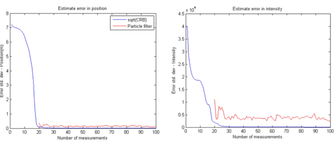
3 robots. The main plot shows the environment where the black dots are the radiation sources and the squares are the robots. The side plots show the corresponding exploration grid maps of each robot. Each exploration grid map shows a robot position (square), partial intensity map (black dot), next frontier cell/current estimated point (yellow diamond), visited area (white) and unvisited area (green). . . 35 5.5 Performance of the particle filter compared with the CR lower

bound. . . 37 5.6 The green line in the radiation map (a) shows the route that

the robot takes to localize the radiation source. The particles in the particles view (b) converges to the source. The map entropy decreases as the iteration increases as expected. . . 40 5.7 Test scenario of intensity estimation algorithms. The top left

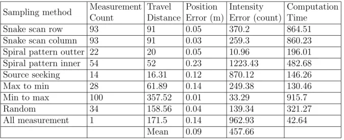
corner is the robot measurement points in magenta. The environment radiation level is indicated by the color (blue = low radiation, yellow = high radiation). The red dot is the intensity estimation location. . . 41 5.8 Sampling methods of radiation estimation algorithms. . . 47 5.9 The comparison between estimation methods and measurement

sampling methods. . . 50

(10)

5.10 Using the source seeking method and multiple landmarks intensity estimation using calculation. We compare between

different memory capacity of the robot. . . 52

5.11 Test scenarios: (a) 4 sources at top right corner, (b) 4 sources at bottom left corner, (c) 9 sources equally distributed. . . 55

5.12 The comparison of position error between the ideal case (0m error), 0.05m, and 0.1m error that were introduced to the measurement reading. . . 56

5.13 The comparison of intensity error between the ideal case (0m error), 0.05m, and 0.1m error that were introduced to the measurement reading. . . 57

5.14 The comparison of measurement count between the ideal case (0m error), 0.05m, and 0.1m error that were introduced to the measurement reading. . . 58

5.15 Algorithms performance in Scenario I. . . 59

5.16 Algorithms performance in Scenario II. . . 60

5.17 Algorithms performance in Scenario III. . . 61

5.18 Comparison between number of robots. . . 62

5.19 Multiple sources experiment: comparison between travel distance vs number of robot with variation in communication range. The vertical bars in the 3 robots case indicate the maximum and the minimum number of travel distance. . . 63

5.20 Inside a configuration spaceC, the algorithm samples nodes in a free space C_{f ree}. Then, the algtorithm will try to connect these nodes to form a graph. The obstacle C_obs is the area that the nodes cannot be connected. . . 64

5.21 Freiburg indoor building 079 as a test map. . . 70

5.22 Node and edge generation of probabilistic roadmap over the map. . . 71

5.23 Frontier cells are generated on free space by removing those frontier cells which are out of bound. . . 72 5.24 Three robots are deployed in the environment. The top figure

is the global map of all robots. The middle maps are the visited (white space), unvisited (green dots) and frontier cells (magenta dots). The bottom maps are the estimated intensity map of each robot. When they are within the communication distance, they are able to share the information about the map e.g.frontier cells, visited and unvisted cells and radiation point. 73

(11)

5.25 Assume that we have the absorber matter that has thickness of x, The initial radiation I₀ on the left hand side will pass through the substance and the reduced intensity I(x) is on the right side as the result. . . 74 5.26 The environment is assume to be indoor with defined boundary.

The robot can spawn anywhere in the environment, also the radiation point. The robot is forbidded to cross the wall. . . . 75 5.27 The grid map created by the robot in order to understand

the free space and occupied area. . . 76 5.28 Probabilistic roadmap created by a robot as a tool to traverse

inside the environment. . . 77 5.29 The plot of the radiation inside the difficult accessible area

(4.5,6). . . 78 5.30 The initial step of the experiment. The robot is placed at

the middle bottom of the environment so the robot will have the difficulty to reach the radiation source inside the difficult accesible space. . . 79 5.31 The robot will travel in the low intensity area and search for

high intensity area. . . 80 5.32 When the robot is in the high intensity area, it will generate

a path to check the estimated intensity point that estimated by particle filter. . . 81 5.33 After the robot has arrived at the estimated area, it will

follow the estimated point and measure the radiation near the estimated point in order to fine tune the estimated location and intensity of the source. . . 82 5.34 The robot will finish the process when the criteria is met. In

this case, if there is no improvement in the result for 5 iteration and the robot has visited the estimated location, the algorithm will end. . . 83

(12)

List of Tables

5.1 Performance comparison of the proposed method vs traditional methods . . . 38 5.2 Single Landmark Intensity Estimation . . . 42 5.3 Multiple Landmarks Intensity Estimation using Optimization . 47 5.4 Multiple Landmarks Intensity Estimation using Calculation . . 50 5.5 Source Separation Algorithm Comparison . . . 53 5.6 Comparison between different in communication range using

real world map. . . 65

(13)

(14)

Chapter 1 Introduction

The environmental hazard is an important threat where chemical substance damages the environment, which has an unfavorable effect on living organisms.

One of the causes that contaminate surroundings is radioactive material leakage, which is an increasing concern in national security [5, 6]. This emerging threat can be either induced by a malicious attack or accidental release of radioactive material. Thus, the radiation source estimation can be a valuable tool in order to plan a counter-measure to the problem, including saving human life and clean up the leakage material [7, 8].

Nowadays, the existing technologies in radiation detection mainly operate manually or stationary [9,10]. The first method is to use human as an explorer by manually waving the radiation detection device in the possible area of radioactive leakage [11]. In this method, the gathered information may not provide the complete visual or statistic data map. In the worst case, the operators may be exposed to the radiation themselves, which can later cause a serious radiation sickness [12]. Another method to detect the radioactive material is to use a stationary portal monitor. This method is mainly used in the port to scan the shipping container or cargo. The drawback of this method is the lack of mobility.

Autonomous robotic systems have become increasingly interested by researchers around the world [13]. The replacement of human force to perform dangerous task such as nuclear radiation detection is the advantage of the robotic systems. In addition, the mobility given by robots can surpass human in the process of data gathering in an inaccessible area by human. Moreover, robots can work together as a team to quickly accomplish the task objective with either centralized or decentralized way. Thus, using robots in the task of radiation intensity mapping is a better choice.

This thesis is divided into 6 chapters. Chapter 1 consists of the introduction. Chapter 2 is the literature review. Next, chapter 3 explains the recursive bayesian estimation and particle filter. Chapter 4 talks about the exploration algorithms for robots. Chapter 5 shows the experimentation and analysis of this research. Lastly, chapter 6 is the conclusion of all works.

(17)

1.1 Problem Statement

The main problem of exploration in the radiation field is the measurement uncertainty [14–16]. Each sensor measurement of the robot at the same position does not guarantee to have the same value. In a particular case, it is based on Poisson distribution. The particle filter is one of the tools that give flexibility over the non-linear system. One way to navigate through the exploration field to locate the radiation source is to follow the estimated source location of the particle filter [17, 18]. However, that does not guarantee to be the optimum path, or the result may be a failure in the worst case due to the distance between the robot and the source. If the location of the robot is far away from the source or in low radiation area, the particle filter does not guarantee to give an accurate result due to lack of information. This work proposed the method for both exploration and multiple sources localization using robotic systems. The minimum cost in exploration can be achieved by moving a robot to the appropriate position. We proposed the algorithm for selecting the next best position by considering several conditions, such as, the minimum distance from the current position of the robot to the available target position and the largest gradient direction. Furthermore, the area pruning algorithms are employed to decrease the exploration cost by avoiding the possibly low intensity area using recursive Bayesian estimation pruning and low priority flag. In addition, for single source case, information gain based exploration has been investigated. The robot will use the information gain-based exploration, which can calculate the best possible action for the robot by using the particles information (weight, intensity, and location).

Finally, after the sources localization is finished, unknown sources intensity separation algorithm will be applied to further increase the measurement accuracy.

(18)

Chapter 2 Literature Review

2.1 Basic Knowledge of Radioactivity

Radioactivity is a process of an unstable atom emits ionization radiation. The atom loses a nucleus in the process. Radioactivity is also known as radiation decay, or nuclear decay. The material which emits radiation is consider a radioactive [19–21].

2.1.1 Type of Radiation

The types of energy that emit from an unstable atom are alpha particle (α), beta particle (β), and gamma ray (γ). Fig. 2.1 shows those particles and their penetration properties.

2.1.1.1 Alpha Particle

Alpha particle is the weakest type of radiation. It consists of two neutrons and two protons which weight about 8,000 times of an electron. It can be shielded by a piece of paper which means it is completely harmless to human when a body get exposed. However, it is only harmful when it is inside the body.

2.1.1.2 Beta Particle

Beta particle is an electron particle which has very light weight around 1/2000 the mass of single proton or neutron. It can be shielded by a wall of wood or aluminium. It is able to penetrate the human skin a little which is not harmful to human in a small dose.

2.1.1.3 Gamma Ray

Gamma ray is the third kind of radiation which is not particle. It is a high energy form of light which has no mass. It has high penetration property

(19)

Figure 2.1: Alpha particle (α), beta particle (β), and gamma ray (γ) with their penetration properties [1].

which mean it can penetrate through almost everything including human body. However, it can be blocked by a thick wall of lead. It is very hazard to living organisms [22].

2.1.2 Radioactivity Measurement

The most common radioactivity measurement is a Geiger counter. It consists of a metallic tube which is filled with a gas. Fig. 2.2 shows how a Geiger counter works. When the device is exposed to the radiation, The atom inside the tube will be ionized by the radiation. The negatively charged electrons (blue particle) are attracted the positively charged anode (red wire) while the positively charged protons (red particle) are attracted to the side of the tube which is a negatively charged cathode (blue wall). A Geiger counter will count the electron that passed the anode wire. The unit of a Geiger counter is count per second (count/s) [22].

2.1.3 Radiation Model

The radiation reading from a measurement device follows the inverse square relationship. The intensity of the radiation source is inversely proportional to the distance relatively to the instrument according to the following equation

(20)

Figure 2.2: The operation inside a Geiger counter [2].

[23]:

λ_k = I

(x_k−x₀)²+ (y_k−y₀)² + (z_k−z₀)² +λ_b (2.1) where λ_k is the intensity at the measurement device. I is the intensity of the source, (x_k, y_k, z_k) is the position of the measurement device, (x₀, y₀, z₀) is the position of the source, andλb is the background intensity at the measurement point. In our case, we use a ground mobile robot and we assume that the intensity source is on the ground. Therefore, the altitudes z_k, z₀ are zero.

However, from the experiment, if the robot moves closer to the source point, the reading becomes near infinity because the different between (x_k, y_k) and (x₀, y₀) is near zero. To solve this problem, we set the altitude different z to

be 1. The new equation is as follow:

λk = I

(x_k−x₀)²+ (y_k−y₀)²+ 1 +λb (2.2) The example plot of the radiation using Eq. 2.2 is shown in Fig. 2.3. For multiple sources case, since there are two or more sources, the intensity model

(21)

Figure 2.3: The example plot of the radiation of the source intensity of 10,000 at the location (0,0). The background intensity is set to 1,000.

equation (Eq. 2.2) cannot be applied to map the source. In this case, we adopt the new intensity model by combining every sources using the following equation:

λ_k = ( _M

X

i=1

I_i

(x_k−x_i)²+ (y_k−y_i)²+ 1 )

+λ_b (2.3)

where λk is the k^th measurement at (xk, yk). M is the maximum number of the source. I_i is thei^th intensity at (x_i, y_i). λ_b is the background radiation.

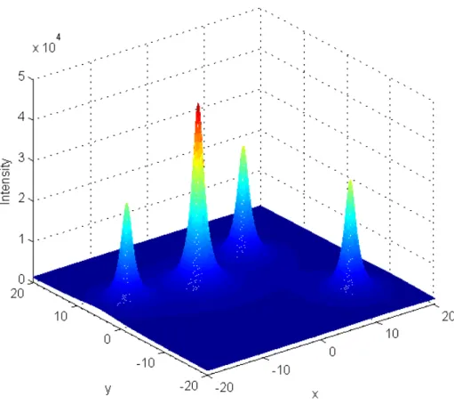
The example plot of the radiation using Eq. 2.3 is shown in Fig. 2.4.

However, each decay event of radioactive is random, independent and occurs at a fixed mean rate λ. [24] describes the model of radioactive decay using Poisson statistics as the following equation:

f(k, λ) = λ^ke^−λ

k! (2.4)

(22)

Figure 2.4: The example plot of the radiation of 4 sources with random intensities. The background intensity is set to 1,000.

where λ = I is the average number of count for that period of time. k is the exact measurement reading from the source. Gaussian distribution can be used to approximate Poisson distribution when λ becomes large (with λ = µ = σ²). Fig. 2.5 shows the uncertainty of measurement vary with distances and graph fitting using Poisson and Gaussian distribution.

We assume that the radiation detector attached to the robot location (x_k, y_k) is uniformly directional response and neglect the air attenuation. The measurement by a robot is independently distributed and the exposure time τ of all measurement is constant. The radioactive are separable point sources and have a finite number of points in a known geometric area without obstacle.

However, the number of sources is unknown by the robot.

(23)

Figure 2.5: A measurement uncertainty of radioactive vary with distances with the graph fitting using Poisson and Gaussian distribution [3].

2.2 Related Works

The radioactive measurement gives a non-linear output [25,26], yet introduces uncertainty in measurement [24]. In order to handle these issues, there are several studies addressing the problem of source localization and estimation.

The radioactive source localization can be achieve using several techniques.

The main categories for localizing the radiation source lies in the single source and multiple sources localization. For a single source localization, the common method is to use radiation reading as signal strength in different locations to determine the possible source in a certain area. [3], [27] utilize this approach by measurement the radiation circularly around the possible intensity source. The author applied three estimation techniques: maximum likelihood estimator (MLE), the extended Kalman filter (EKF), and the unscented Kalman filter (UKF). The Cram´er-Rao lower bound was used to find the lower bound for estimation algorithms. The MLE gave the best result among other methods, but the computational intensive is the problem of this algorithm. It is unlikely that MLE can be used in real-time application. The EKF and UKF gave inaccurate result. The EKF, moreover, diverged from the CRLB. The test was done on both simulated source and trial data.

Similar technique of MLE was used in [28] to detemine multiple sources by measuring the source from the distance which the number of source, intensity strength and location are unknown. The author managed to estimate the source location using MLE and use generalize maximum likelihood to find the

(24)

number of souces. Another technique is to estimate the sources parameters using particle filter using important sampling with a progressive correction.

The author successfully estimates 0-2 sources but from three sources onward, it was not very good using MLE. Bayesian estimation perform well in both cases.

[29] use the concept similar to global positioning system calculation by finding the level curves of the sources using the detector placed in the corner of the room. Thus, they said the intersection point has the highest probability that the source exist. The recursive least square optimization was used to estimate the sources from different sensors. However, the source intensity is claimed to be known as a priori. They successfully utilized realtime tracking of the source with some error in an indoor environment.

One of the interesting approaches is to use a vehicle to carry a detection device for measuring the intensity. [4] used a helicopter to carry a detector and flew over the area to localize the radiation source. The particle filter was used as the localization technique with a prior knowledge of the intensity of the source type of 1/R². [30] used a mobile ground robot equipped with a detector to localize a source. There are obstacles in the environment and the author used the artificial force field algorithm with the control vector to avoid them. As a result, the smooth path was generated and the robot successfully located the source.

The multi sensor approach is presented in [31]. The author used a group of mobile robots with detectors to map the radiation over a given polygonal area.

Each robot is capable to share the measurement information and its location with another robot using wireless communication. The search environment was divided into a grid map. The robots will follow the information gradient and map the radiation by measure every grid cell. The test was done using a red LED as a simulated source.

For multiple radiation sources localization, [32] presents glowworm algorithm for a swarm of robots for multiple sources localization. The glowworm optimization is a well-known algorithm for localize the local optima of function.

The agents in the algorithm carry a luminescence quantity called luciferin, which used to for information sharing. The agent will vary its sensor range parameter in order to compute its movement and move toward the one that has higher luciferin then its own. The author adapted the glowworm optimization for the case of radiation sources localization. It is successfully run with a swarm of 100 agents. The achieve minimum distance between two sources is 0.39m.

Another interesting technique for multiple sources localization is the contour tracking technique as in [23]. The author used a helicopter that equipped with the measurement device. The helicopter flew in the radiation

(25)

field by tracking its contour at low intensity measurement. Since the shape of the radiation that emits from the source is a circular shape. The contour of a single source is circle. For multiple sources, the Hough transform is used to determine multiple circles, in order to find the centers of the circles, which leads to the source locations. The limitation of the helicopter is that the fuel burns very fast. The author managed to swiftly tracking contour and provided a rough estimation of the radioactive sources.

In an intense radiation field, it is possible to locate the radioactive source by letting a robot follows the intensity gradient. However, if the robot is a long distance from the radiation source, the intensity measurement will be weak.

Thus, a robot needs an exploration algorithm to efficiently locate the strong measurement which will lead it to the source. In addition, the exploration time might be constrained since there is limited measure of battery and limit evacuation time. Thus, an efficient exploration scheme for a robot must be utilized, which should minimize the exploration cost (e.g. traveling distance, time) but maximize the information for a robot. For exploration strategy, [33]

presented the frontier-based exploration algorithm by directing robots to a region, called frontier cells, which lies between known and unknown areas.

The algorithm is able to fully explore a reachable workspace and generate a reachability map [34, 35]. A robot will use appropriate criteria for choosing the best frontier for the best performance. The common criterion is the minimum distance from a robot to the frontier cell. However, it depends on the environment that additional criteria may be applied (e.g. terrain type, path cost, input measurement).

(26)

Chapter 3 Radiation Estimation Algorithm

Due to the fact that the reading of a measurement device is uncertain as discuss in Section 2.1.3, the gradient-based methods may not work because they do not consider sensor uncertainty [36]. Thus, the estimation algorithm is needed to tackle the problem of noisy measurement.

3.1 Recursive Bayesian Estimation

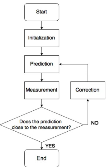
Recursive Bayesian estimation (RBE) or Bayes filter is an excellent method to deal with sensor uncertainty [37, 38]. It also provide the real-time computational feasibility with localization accuracy [9, 39]. Most recursive Bayesian estimations have the same concept which is to predict the system behavior by using the measurement to correct the prediction following Bayes theorem:

P(x|z₁, . . . , z_n) = P(z_n|x, z₁, . . . , zn−1)P(x|z₁, . . . , zn−1)

P(z_n|z₁, . . . , zn−1) (3.1) where x is the estimated state. z is the observation as the measurement.

The left hand side of the equation is P(x|z1, . . . , zn) which is the posterior belief. It is the product of the measurement model P(z_n | x, z₁, . . . , zn−1) and the prior belief P(x|z₁, . . . , zn−1) divided by the normalization constant P(zn |z1, . . . , zn−1).

Recursive Bayesian estimation start with the initial state. Next step is the prediction step, it will update the belief space. Then the measurement step, the prediction is corrected using the measured data [40]. The process will repeat at the prediction step and will converge when the prediction is close to the measurement. Fig. 3.1 shows the basic of recursive Bayesian estimation operation. There are two kinds of belief space in recursive Bayesian estimation. The first one is the bell-shape belief space called Gaussian belief space as in Fig. 3.2. The Kalman filter utilizes this kind of belief space due to the fact that it has only two parameters; mean and covariance. Another one is the non-Gaussian belief space which has an arbitrary shape [41, 42].

(27)

Figure 3.1: Overall process of the recursive Bayesian estimation algorithm.

This belief space suits for recursive Bayesian estimation algorithms like the particle filter because the filter has particles which have random attributes and each of them represent a single belief. The plot of these beliefs can be any shape, for instance in Fig. 3.3. The grid-based method and element-based method are also suit non-Gaussian belief space. the In this work, we use the non-Gaussian belief space because a single static sensor measurement of a source intensity cannot be used to determine the source location directly.

The non-Gaussian belief space would provide a ring-like shape which tells us where the source may locate.

Each recursive Bayesian estimation algorithms comes with different performance in efficiency, ability for non-Gaussian, and ability for non-linearity as in Fig.3.4. The simplest algorithm of recursive Bayesian estimation is the Kalman filter (KF). It is the most efficient but perform poorly in non-Gaussian

(28)

Figure 3.2: A Gaussian belief space.

system and it is a very linear process model [43, 44]. The extended Kalman filter (EKF) uses the Jacobian matrix to relax the linear constraint but it still suffer from non-Gaussian distribution [45, 46]. The unscented Kalman filter (UKF) allows some non-Gaussian belief space but does not work well with highly non-linear and non-Gaussian system [3, 47]. The grid-Based method (GM) has the performance depends on the selection of grid mesh or the number of elements and it suffers from computational complexity because the convolution of motion and measurement update e.g. the 3-D grid update requires 6-D operation [48–50]. The same reasons go for element-based method (EM). The most compromise of efficiency and performance for non-linear and non-Gaussian system is the particle filter (PF) [51]. In addition, the particle filter is non-parametric, thus it provides heuristic and more flexibility than other algorithms [52–55]. Therefore, it is used for intensity mapping algorithm in this work.

(29)

Figure 3.3: A non-Gaussian belief space.

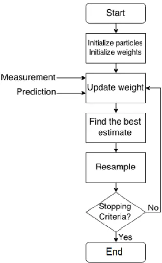
3.2 Particle Filter

In this work, we choose the particle filter as the mapping algorithm since it compromises efficiency and performance for the non-linear and non-Gaussian systems [56, 57]. In addition, the particle filter is non-parametric. Thus, it provides heuristic, and it is more flexible than other algorithms [58, 59]. The particle filter or Sequential Monte Carlo (SMC) is the method representing the posterior belief using a set of random state samples as particles [60].

Each particle is basically a hypothesis of the real state at time t with an associate weight to represent the accuracy of the hypothesis based on the state measurement. The detail of the particle filter algorithm is in Algorithm 3.1. The particle filter starts with initialization of random hypothesis states as initial particles with equally associated weights. Then, the error model is used to find the error between measurement and prediction. The weight of each particle will be updated by the product of the weight of previous time step and the likelihood function. The likelihood function comes in the form of the normal distribution of the error with mean µ and variance σ. The

(30)

Figure 3.4: Recursive Bayesian estimation algorithms comparison [4].

weight must be normalized so they sum up to 1. The estimated state will be calculated by state estimate model. Some of the lowest weight particles will be resampled at the high weight particles at resampling step. Finally, the particles and the weights will be updated to be used in the next time step.

3.2.1 Target State

We use mobile robots to explore and map the radiation. The estimation state xfor each particle requires the location (x, y) of the source and its intensity I as:

x=

x y I

(3.2)

3.2.2 Intensity Estimation of Particles

We can use Eq. 2.2 to calculate the particle expected intensityIat the location (x, y) as we have ak^thmeasurementz_kat the robot location (x_k, y_k). However, it may introduce an estimation accuracy problem since we only use the current measurement that only provides the information at a specific location. If we combine the previous measurements, which include measurement locations

(31)

Figure 3.5: Overall process of the particle filter.

(x_1:k, y_1:k) and intensity measurement λ_1:k, the particles’ intensity estimation will be more accurate.

3.2.2.1 Single Landmark Intensity Estimation

From Eq. 2.2, we can estimate the particle’s intensity Iⁱ at (xⁱ, yⁱ) using the current measurement z_k by:

Iⁱ

d²_k +λ_b =z_k (3.3)

where d_k = p

(x_k−xⁱ)²+ (y_k−yⁱ)². However, the drawback of single landmark intensity estimation is that, the current measurement does not estimate the intensity quite well. The reason is because the measurement

(32)

Algorithm 3.1 Particle Filter

1: Initialize particles: x₀ =rand(N,1)

2: Initialize particles’ weights: w₀ = 1/N

3: while Not converge do

4: errorⁱ =error model(measurementⁱ, predictionⁱ)

5: for i= 1 to N do

6: Update weight: wⁱ_k=wⁱ_k−1·likelihood f unction(errorⁱ)

7: end for

8: Normalize weights: w = PN^w i=1wⁱ

9: Calculate state estimate: ˆx=state estimate model(w, x)

10: Resampling process

11: Update particles: x_k+1 =x_k

12: Update weights: w_k+1 =w_k

13: end while

error from sensor worsen the estimation. Thus, using multiple estimation points can improve the measurement drastically.

3.2.2.2 Multiple Landmarks Intensity Estimation Algorithm

Optimization method To get more accurate estimation of the intensity point Iⁱ is to use all n measurement z_k−n, . . . , z_k. Optimization algorithm is one of the method to achieve this goal. In this work, we want to show you the example of using an optimization algorithm to determine the estimation intensity. The algorithm that we choose is the nonlinear program solver in MATLAB called fmincon, which specify the constrains and function by:

minx f(x) such that











c(x)<0 ceq(x) = 0 A·x≤b Aeq·x=beq lb≤x≤ub,

where c(x) and ceq(x) are the subject of minimization of inequality and equality of nonlinear function respectively. A·x≤bandAeq·x=beq subject to the minimization of linear inequality. lb andub are lower bound and upper bound of x. For this work, we only require lb and ub parameters for intensity Iⁱ. The rest of the parameters are empty. The objective function is the likelihood function equation (Eq. 3.14) in section 3.2.3.

(33)

However, the drawback of the optimization method is the computational time. Since it requires intensive calculation from the lower bound lb to upper bound ub of every particle, the computation time increases directly proportional to the number of particles.

Calculation method From section 3.2.2.1, consider the previous measurements from the first measurement to measurement n, they also can estimate the intensity Iⁱ by:

Iⁱ

d²_k +λ_b =z_k (3.4)

Iⁱ

d²_k−1 +λb =zk−1 (3.5)

Iⁱ

d²_k−n +λb =zk−n (3.6)

combining those terms, we have:

Iⁱ

d²_k +λ_b+ Iⁱ

d²_k−1 +λ_b +· · ·+ Iⁱ

d²_k−n +λ_b =z_k+zk−1+· · ·+zk−n (3.7) Iⁱ

d²_k + Iⁱ

d²_k−1 +· · ·+ Iⁱ d²_k−n =

n

X

j=0

(zk−j −λ_b) (3.8) Iⁱ·(d⁻²_k +d⁻²_k−1+· · ·+d⁻²_k−n) =

n

X

j=0

(z_j −λ_b) (3.9) Iⁱ·

n

X

j=0

d⁻²_k−j =

n

X

j=0

(zk−j −λ_b) (3.10) Iⁱ =

Pn

j=0(zk−j−λ_b) Pn

j=0d⁻²_k−j (3.11) Thus, Eq. 3.11 can be used to estimate the particle’s intensity Iⁱ using previous and current measurements.

3.2.3 Likelihood Function

By using Eq. 2.4, we can calculate the likelihood x_i of particle i by using the k^th measurement z_k and the predicted intensity λⁱ_k from Eq. 2.2, in the case of single landmark estimation. Here, we approximate the Poisson distribution to the Gaussian distribution to reduce the computational complexity [3]:

(34)

p(z_k;xⁱ) =P(z_k;λⁱ_k) (3.12)

≈ N(z_k;λⁱ_k, λⁱ_k) (3.13) In the case of multiple landmarks estimation using the previous and current measurements z_1:k at (x_1:k, y_1:k), the new likelihood function is the product of all likelihoods from all measurements as:

p(z_1:k;xⁱ)≈

k

Y

j=1

N(z_j;λⁱ_j, λⁱ_j) (3.14)

where z_k is the measurement update from the robot at time step k. xⁱ is the current state of the particle i which is used to calculate the predicted intensity λⁱ_k at the robot location using Eq. 2.2 as follow:

λⁱ_k= I_i

(x_k−x_i)²+ (y_k−y_i)² +λ_b (3.15) where (x_k, y_k) is the robot position at time step k. I_i is the intensity of the particle i. (x_i, y_i) is the location of the particle i. λ_b is the background radiation. The Poisson distribution is approximated as the Gaussian distribution by µ=σ² =λ_k.

The state estimation of the particle filter is usually the average state of the particles with the highest weights. If the portion of the top particles is too high, the algorithm may not converge. If the portion is too low, the algorithm may converge to the wrong location.

3.2.4 Resampling Process

The resampling process is on how to remove the lowest weight particles and resample them elsewhere in order to avoid the problem of degeneracy [61].

The degeneracy problem is the usual problem in the particle filter, which is a few highest weight particles dominate the distribution while most particles will have weights close to zero [62]. The resampling process will remove a portion of the lowest particle weights and resample them at the high weight particles using the roulette wheel selection [63, 64]. In addition, the particles that have zero weight will be resampled as well. It is to ensure that some of the high weight particles will be selected and also add diversity to the

(35)

population from lower weight particles. The newly born particles x^index

j L

k+1 will have the a uniform weight as:

w_k^index^L =U(1/N) (3.16)

where w^index_k ^L is the low weight particles with index indexL, and N is the number of particles. The Gaussian noise is applied to the portion of those which are resampled near the high weight particles x^target_k to increase the diversity as in the following equation:

x^index

j L

k+1 =x^target_k +N(µ, σ²) (3.17)

wherex^index

j L

k is the low weight particle j. x^target_k is the selected target of high index using the roulette wheel selection. randnis the Gaussian noise with the mean µ= 0 and the standard deviation σ is mag. However, as the process continues, the standard deviation of the noise mag becomes linearly lower overtime to make the algorithm converge. When the measurement is higher than the detection threshold, the robot will pretty much know which area contains the source. Thus, resample the particle at the estimated states will accelerate the convergence process.

3.2.5 Termination Criteria

The algorithm will converge when the termination criteria are met. In this case, we set the termination criteria as: if the root mean square error of the estimated intensity is less than 5% for 5 iterations and if the robot has visited the area within 1.5m around the estimated location, the algorithm has converged. The reason why the robot has to visit the estimated location is to prevent the algorithm from ending too soon, which may lead to the false location of the radiation source.

(36)

Chapter 4 Exploration Algorithms

4.1 Frontier-base Exploration

In order to explore the environment, the robot needs to know which part of the area is not visited and which part is visited. By knowing visited and unvisited area, the robot will not have to move to the same location, thus it gives an efficient exploration [65]. Frontier-based exploration is the excellent tool for a robot exploration. It uses a grid map to determine visited and unvisited area. The cells between visited and unvisited area are called frontier cells, which the robot uses to determine where to go next [33, 66–69].

Fig. 4.1 shows how a robot creates grid map. The white area is the area that has already been visited by the robot. The green area is the area that has not been visited by the robot yet. The blue asterisks are the frontier cells.

4.1.1 Target Point Selection

To determine the direction of a robot, an algorithm for choosing an appropriate frontier cell is needed. We will use a cost function to determine the for the robot using the following criteria:

1. Intensity gradient: the robot will choose the frontier in which the intensity measurement tends to be higher by following the direction of increasing intensity gradient.

2. Distance: the robot will calculate the Euclidean distance from itself to the frontier.

The minimum-cost path is computed using the following equation:

V_tⁱ =α||i−t||+ (1−α)D(ax₀+by₀+c,(t_x, t_y)) (4.1) where V_tⁱ is the cost of a robot i_x,y to reach frontier position t_x,y. α is the importance weight of the distance and the intensity gradient which set between [0,1]. From experiment, we set α = 0.8. The intensity gradient

(37)

Figure 4.1: Left side, the simulated environment with a robot represented by a square. Radiation sources are represented by black dots. Small dots with color indicate the particles with associate weights. Right side, The robot grid map with visited area (white), unvisited area (green) and frontier cells (asterisks).

can be achieved by using the past and current measurements of a robot.

D(ax₀+by₀ +c,(x, y)) is the distance from a frontier position (x, y) to the gradient line ax0 +by0+cas in Eq. 4.2.

D(ax0+by0+c,(tx, ty)) = |at_x+bt_y+c|

√a²+b² (4.2)

whereax0+by0+c is the line equation of the gradient direction and (tx, ty) is the position of a frontier cell.

4.1.2 Area Pruning

To create an accurate map, the robot needs to visit every cell in the grid map.

However, a small isolated unvisited cell that is surrounded by explored cells with low intensity can be ignored because it gives low exploration gain. In addition, a source is unlikely located in that area because the surrounding cells are examined. We can apply Eq. 2.2 to find the possible intensity of that cell, if it is lower than the detection threshold, it can be ignored, thus, explored. The situation like this usually happen by chance. In our case, we will assume that some frontier cells are not worth to visit. We intentionally skip some frontier cells and flagged them as low priority cells in order to

(38)

examine the surrounding area. The flagged frontier cells are not adjacent to each other. As a result, we can increase the chance that the cells are automatically avoided as we explored.

Every unvisited cells in the grid map can still potentially be ignored. We introduce the cells’ weight by applying recursive Bayesian estimation (RBE).

The intention of this algorithm is not to find the radioactive sources, but it determines which cells has low value as a robot travel and measure the intensity along the way. RBE uses the same technique as PF (Eq. 3.13) to determine the weight of each cell. Thus, if the measurement is decreasing as the robot moves toward one cell, that cell could be ignored because the probability of finding a source in that cell is low. However, the low weight cells can only be remove when the robot moves close to that cells, to prevent the problem of over pruning, since a single measurement cannot determine the whole weight of all cells. In addition, the algorithm will not work in the high intensity area (e.g. near the sources) because it will be come a source searching algorithm instead, which is the task of the particle filter.

Fig. 4.1 also shows the cells those are marked with low priority flags () and all unexplored cells are assigned with weights.

4.1.3 Multi-robot Systems Extension

From a single robot, we can extend our work to muti-robot systems by adding one or more robots to the workspace. Each robot can communicate to exchange information, including grid map, partial intensity map, and the current source estimation. However, in some cases, two or more robots choose the same frontier cell which is not the optimal solution. To prevent this, robots will compute the utility of frontier cells U_t [70]. Initially, each frontier cell t will have the utility U_t set to 1. Once a robot choose a frontier cell t⁰, the utility of that frontier cell and adjacent frontier cells in distance d from t⁰ are reduced by P(d). Thus, the utility U(t_n|t₁, ..., tn−1) of a frontier cellt_n given that the frontier cells t₁, ..., t_n−1 are assigned to the robots 1, ..., n−1 is computed by

U(t_n|t₁, ..., tn−1) =U_t_n −

n−1

X

i=1

P(||t_n−t_i||) (4.3) If there are many robots which choose the frontier cellt_n, the utility of that cell tends to be low. In our case, the environment is known and has no obstacles. P(d) is set to be the normal distribution with µ= 0 and σ = 0.4, so the utility of the target frontier cell t_n will be close to 0.

(39)

Algorithm 4.1 Target Point Selection

1: Determine frontier cells of all robots

2: Compute the cost V_tⁱ for each robot

3: Set the utility U_t = 1 for all frontier cells

4: while there is a robot without a target point do

5: Determine a roboti and a frontier t that satisfy:

(i, t) = argmax_(i⁰_,t⁰₎U_t−γV_tⁱ

6: Reduce the utility of the selected frontier cell and adjacent frontier cells byU_t⁰ ←U_t⁰ −P(||t⁰ −t_n||)

7: end while

By considering a trade-off between the cost of moving to the target frontier cell V_tⁱ and the its utility U_t, the target point selection can be calculated using Algorithm 4.1.

From Algorithm 4.1,U_t−γV_tⁱ is used to find the roboti and the frontier t which give the best evaluation. The process continues iteratively until all robots choose their frontier cells. γ ∈[0.01,50] gives the importance of cost versus utility. It is set to 1 in this case.

When any robots discovers any neighbors, they will start sharing information to each other. The exchange information process aims to reduce the exploration time. Thus, there are several crucial information to be shared, which are the current source estimation, exploration map, and partial intensity map. The current source estimation is shared among neighbors in order to increase the converging process. When two or more robots have the same source estimation, the robot will accelerate the termination process. To reduce the exploration time, the unvisited grid maps of robots will intersect and the intersection part could be where both robots have not visited. Another piece of information to share is the partial map of the sources discovered by each robot. The partial intensity maps of each robot will be merged so each robot knows the locations of the sources that have already been discovered. The merging process is to compare discovered sources with each other. If there are any new sources from other robots, the sources will be added. If there are sources which are already discovered, the position and intensity of any duplicate sources will be averaged.

4.2 Information Gain-based Exploration

The entropy is the tool to measure the uncertainty of a random variable [71,72].

In this case, we want to evaluate the uncertainty of the map using the entropy

(40)

to model this in the probabilistic manner [73].

H[P(x)] =− Z

x

p_ilogp_i (4.4)

≈ −

n

X

i=1

p_ilogp_i (4.5)

where, p_i = P(x = x_i). In our case, the particle filter entropy is as the following equation:

H[P(x|z_t)] =−

#particle

X

i=1

w_ip(x_i|z_t) logp(x_i|z_t) (4.6) where, xis the distribution of the particles. w_i is the weight of each particle i. z_t is the observation that we obtain at the time step t. Then, the action of the robot a_t can be evaluated using the expected information gain. It is the change of the entropy for the particle filter when we apply the action as:

I(ˆz, a_t) = H[P(x|z_t)]−H[P(x,x|aˆ _t,z)]ˆ (4.7) where ˆz is the observation to be obtained when action a is taken. This value can be calculated by Eq. 2.2, using the estimated intensity value from the current particle filter time step t. ˆx is the new distribution of particles introduces by the action a_t. The expected information gain can be obtained by integrating all the possible measurements ˆz when the robot takes action a_t.

E[I(a_t)] = Z

ˆ z

p(ˆz|a_t, z_t)I(ˆz, a_t)dz (4.8) However, to compute the expected information gain is usually a complicated task. Instead, the utility function using the greedy aspect of the maximum information gain I when the robot takes action a as:

a^∗ = argmax

a

H[P(x|z_t)]−H[P(x,x|a,ˆ z)]ˆ (4.9) The utility function becomes:

U(a) =I(a)−αcost(a) (4.10)

where α is the weight of the cost of the action a that the robot has to take.

We choose the best action, i.e., the action that gives the highest utility as the robot action. The robot will evaluate the available adjacent cells around

(41)

Figure 4.2: The simulated environment with a robot represented by a green square. The small squares that follow the robot are the previous reading in the last two time steps (k −1, k−2). The real location of the source represented by the red circle and the background of the map represents its corresponding radiation level. The estimated location of the radiation source by particle filter represented by the yellow circle.

the robot, at most 8 cells, to calculate the utility of those cells and choose the highest utility as the next action.

Fig. 4.2 shows the overall radiation map that the robot has to explore.

The radiation map is the map with different radiation levels corresponding to the radiation source. According to Eq. 2.2, radiation intensity will reduce inversely proportional to the distance from the radiation source. Fig. 4.3 shows the particles of the robot that are the possible location of the source.

However, as the robot progress through the area, the entropy of the map becomes less and less significant, according to Fig. 4.4. On the opposite, when the robot is getting closer to the radiation source, the particle filter estimation becomes more accurate. Thus, in order to get an accurate result,

(42)

Figure 4.3: The particles of the robot that represents the hypothesis of the source. The white area with no particle is the area that the robot already visited with low information, so the particles in the particular area are resampled elsewhere on the map.

(43)

Figure 4.4: The entropy value vs iteration when the robot explores the radiation field. The entropy value decreases as the iteration increases, which means the information that we gain from the map is lower after each iteration.

the robot should switch to use the particle filter estimation as the target, and takes the action that makes the robot get closer to the target.

4.3 Unknown Sources Intensity Separation

A robot will move to the target frontier until the measurement is higher than a certain threshold. Then, a robot will use the particle filter to estimate the source. The source will be determined sequentially and a robot will use discovered sources to create a partial intensity map using Eq. 2.3. Then, a robot will subtract the intensity of sources of the partial map from the measurement in the real world, using the following formula:

z_k⁰ =z_k−

M⁰

X

i=1

I_i

(x_k−x_i)²+ (y_k−y_i)² (4.11) where z_k⁰ is the k^th measurement subtracted by the partial map. zk is the original k^th measurement at (x_k, y_k). M⁰ is the number of source that the robot has discovered so far. I_i is the i^th discovered source at (x_i, y_i).

From Eq. 2.3, a source is created and summed with other sources of different location and intensity. Thus, each source will add some intensity to each other according to this equation:

I_i⁰ = ( _M

X

j=1

I_j

(x_i−x_j)²+ (y_i−y_j)² )

+λ_b (4.12)

where I_i⁰ is the i^th output intensity source at (x_i, y_i). M is the number of intensity points. I_j is the intensity point at (x_j, y_j). The estimated intensity

(44)

from particle filter is the measurement of I_i⁰. If the robot uses the direct measurement, the intensity map created by the robot will be inaccurate. To solve this, we need the intensity correction algorithm. We know that:

I₁⁰ =I₁+ I₂

d²_1,2 +· · ·+ IM

d²_1,M +λ_b (4.13)

I₂⁰ = I₁

d²_2,1 +I₂+· · ·+ IM

d²_2,M +λ_b (4.14)

... I_M⁰ = I₁

d²_M,1 + I₂

d²_M,2 +· · ·+IM+λ_b (4.15) whereI₁⁰, I₂⁰, . . . , I_M⁰ are the sources which have influence from other sources.

I₁, I₂, . . . , IM are the original sources without influence from other sources.

di,j is the Euclidean distance from pointi to point j. We know I₁⁰, I₂⁰, . . . , I_M⁰ from the measurement and also the location of each source which can be used to calculated d_i,j. Only I₁, I₂, . . . , IM are unknown. Thus, there will be M unknown variables with M equations which are linear equations. The Gauss-Jordan elimination can be used to solve this as: