Memory Saving Feature Descriptor Using Scale and Rotation Invariant Patches around the Feature Ppoints

(1)

LETTER

Memory Saving Feature Descriptor Using Scale and Rotation Invariant Patches around the Feature Ppoints

Masamichi KITAGAWA^†a),Nonmember andIkuko SHIMIZU^†b),Member

SUMMARY To expand the use of systems using a camera on portable devices such as tablets and smartphones, we have developed and propose a memory saving feature descriptor, the use of which is one of the essential techniques in computer vision. The proposed descriptor compares pixel values of pre-fixed positions in the small patch around the feature point and stores binary values. Like the conventional descriptors, it extracts the patch on the basis of the scale and orientation of the feature point. For memories of the same size, it achieves higher accuracy than ORB and BRISK in all cases and AKAZE for the images with textured regions.

key words: image matching, feature descriptor, keypoints

1. Introduction

Portable devices have been equipped with high performance multi-core processors and cameras which can capture very high quality images in recent years. Therefore, many device applications that use cameras have been developed.

Even though the devices show very high performance, they have much smaller main memory size and storage size than PCs. Consequently, memory-saving methods are useful for many portable device applications.

Using feature descriptors is one of the most important techniques in image matching. However, many descriptors that have been proposed in the literature require large memory size. The most famous feature descriptors are Scale In- variant Feature Transform (SIFT)[1] and Speeded-Up Ro- bust Feature (SURF)[2], which describe the gradient vector of pixels and have been used in many applications. These descriptors achieve robust image matching and have rela- tively high ability to describe the feature point because they are rotation and scale invariant. However, they require large memory size.

Randomized tree[3]and Ferns[4]descriptors use possible transformations to transform the patch around the feature point and store binary values by comparing pixel values in the patch to describe possible patch appearances. They require smaller memory size than feature descriptors like SIFT and SURF. However, to enhance robustness for scale and rotational changes, they have to store the compared values by using all possible transformations.

Manuscript received August 18, 2018.

Manuscript revised November 30, 2018.

Manuscript publicized February 5, 2019.

†The authors are with the Graduate School of Engineering, Tokyo University of Agriculture and Technology, Koganei-shi, 184–8588 Japan.

a) E-mail: [email protected]

b) E-mail: [email protected] (Corresponding author) DOI: 10.1587/transinf.2018EDL8176

On the other hand, some feature descriptors based on the binary values[5]–[9]compares pixel values in the patch around the feature point which is normalized the direction and direction. Binary Robust Independent Elemen- tary Features (BRIEF)[5], Binary Robust Invariant Scalable Keypoints (BRISK)[6], Features from Accelerated Seg- ment Test (FAST)[7] binary descriptor based on BRIEF (ORB)[8], Fast Explicit Diﬀusion for Accelerated Features in Nonlinear Scale Spaces (AKAZE)[9]are widely used in recent years. In these methods, the extracted normalized patch contains rather simple pixel value patterns, for example, pixel values changes monotonically and the description ability of the patch is not enough in these method.

This paper describes a memory saving feature descriptor we have developed and propose. It compares pixel values of the points randomly selected in the scale and rotation invariant patch around the feature point by utilizing the scale calculation and feature point orientation in SIFT[1].

In our method, to enhance the ability of the description of the patch, pixel values of all combinations of the selected points in this patch are compared as shown in Fig. 1 because all compared values are related each other. On the other hand, in the conventional methods, the pixel values of the selected points in the patch are compared independently as shown in Fig. 2. In addition, the size of our invariant patch is larger than those of the conventional methods and the pixel

Fig. 1 Comparison of the pixel values in our method.

Fig. 2 Comparison of the pixel values in the conventional methods.

Copyright c2019 The Institute of Electronics, Information and Communication Engineers

(2)

values are aggregated by downsizing the size of the normalized patch to the fixed size to increase the ability of the description.

In the same way as other feature descriptors, ours matches the feature point by using three processes: feature point extraction, feature point description, and similarity evaluation. Its feature point extraction process is the same as SIFT’s but its feature point description and similarity evaluation processes are diﬀerent.

In the following sections, we will explain the feature point extraction algorithm in Sect. 2, our feature point descriptor in Sect. 3, and the similarity evaluation process in Sect. 4. In Sect. 5 we will show experimental results we obtained by comparing our descriptor with conventional methods for diﬀerent memory sizes.

2. Feature Point Extraction

In this section, we will briefly explain our descriptor’s feature point extraction process, which as has been noted is the same as SIFT’s[1].

In the first step, we select keypoints as feature point candidates. A Gaussian pyramid is computed by the convo- lution of Gaussian filters with different standard deviations σ. Then, the Difference of Gaussian (DoG) is obtained by differentiating the outputs of Gaussian filtering with adja- cent scales whose size is normalized by down sampling. Fi- nally, DoG outputs are searched for local extrema over scale and space. The local extrema whose values are larger than the threshold are selected as keypoints with their scales.

In the second step, the feature point is localized to obtain more accurate position of the extrema and determine their orientation. First, in the same way as with the Harris corner detector, the corners are selected on the basis of Hessian matrix eigenvalues. Keypoints whose eigenvalue ratio is larger than a threshold are eliminated because they would be on the edge. Keypoints are also eliminated when the contrast around the feature point is low. Then, the sub- pixel position of the feature point is estimated by fitting the quadratic function around the approximate keypoint. Fi- nally, the orientation of the feature point is determined by creating a histogram of the gradient directions with 36 bins covering 360 degrees in the selected scale. The highest peak in the histogram is chosen as its orientation. Any peak above 80% of the highest one is also recorded as its orientation.

3. Feature Point Description

In this section, we will explain our description of the feature point with its intrinsic scaleσand orientationθ.

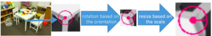
The size S of the squared patch extracted around the feature point is equal tos×σand the direction of its side is parallel to the orientationθ(Fig. 3). Note that this patch is scale and rotation invariant. The extracted patch is scaled to a fixed size (N×N) for size normalization. To reduce the noise, ak×kGaussian filter is applied to the patch.

The feature vector of the normalized patch is calculated

Fig. 3 The normalized patch around the feature point is extracted on the basis of the scale and orientation of the feature point.

Fig. 4 The prefixed positions of the points are distributed uniformly in the normalized patch (red, blue and green circles) and all combinations of the points are evaluated. Selected points for evaluating pixel values are marked as red and blue circles.

by comparing the pixel values of two points whose positions are selected in advance randomly. We compare all possible combinations of two points. In Fig. 4, the pixel value of the red point and that of the blue point are evaluated. If the pixel value of the red point is larger than that of the blue point, feature value 1 is stored; otherwise, feature value 0 is stored. The positions of the pixels for comparing pixel values in the normalized patch are generated according to the uniform distribution to represent the various patterns of pixel values of the normalized patch.

The memory size of our feature descriptor is controlled by the number of points in the normalized patch generated in advance. Even when the number of points is small, our feature descriptor may cover uniformly in the normalized patch because the positions of the points for comparing pixel values are distributed uniformly over the normalized patch. The number of combinations isM(M−1)/2, where the number of points in the normalized path is equal toM.

Therefore, the memory size for our feature descriptor is only M(M−1)/2 bits when the number of points in the normalized path is equal toM.

4. Feature Point Matching

In this section, we will show how our descriptor matches two feature points by evaluating the similarity between feature vectors.

The descriptor evaluates the similarity between two feature vectors by Hamming distance. For the point in interest, we first calculate the Hamming distance from the point in interest to all the target points and then select the point that has the smallest Hamming distance for its corresponding point.

Because our feature descriptor is a binary sequence of lengthM(M−1)/2, where the number of points in the normalized patch is equal to M, similarity between two fea- ture vectors is calculated by logical AND of the binary se- quences.

(3)

5. Experiments

In this section, we will show the experimental results obtained by changing the parameters in our method and compared with the conventional methods.

5.1 Experimental Environment

In the experiments, we used a PC with an Intel Core i3 CPU, a 12 GB memory and a Windows 10 OS. The language used in the experiments was MATLAB and C++. Our method was implemented using MATLAB. The SIFT source code provided by Lowe[10]was used for the feature point extraction in our descriptor. The source codes for BRISK[6], ORB[8], and AKAZE[9]were used in the experiments provided in OpenCV in comparison with our method.

The image pairs “Adirondack”, “Vintage”, ”Pipes”,

“Teddy”, and “Piano” from the Middlebury stereo data- sets[11]are used in the experiments. For the image pairs

“Adirondack” and “Vintage”, we used four types of image pairs: the original pairs with occlusion, the pairs in which one of the images was rotated by 5^◦ from the original image, the pairs in which one of the images was scaled by 0.8 from the original image, and the pairs in which both of the images were added 1% salt and pepper noise. For the image pairs “Pipes”, “Teddy” and “Piano, we used the original image pairs. Example of the image pairs “Adirondack” used in the experiments are shown in Fig. 5.

5.2 Evaluating of the Results

The matching results between the pairs of images were evaluated on the basis of the distance between the ground truth positions calculated by the transformed position and the positions of the matched points. We assumed that the result was true matching when the Euclidean distance was less than 2.5 pixels. We evaluated the accuracy, which is the

Fig. 5 Examples of the image pairs used in the experiments.

proportion of the true matching results obtained.

5.3 Experiment 1: Parameters in Our Method

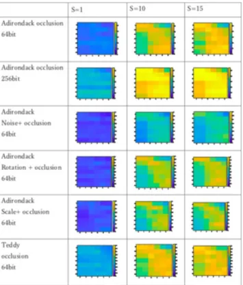
In this section, the results are shown by changing the scale Sof the extracted patch was equal toS=1, 10, and 15. The size of the normalized patch was changed fromN×N=5×5 to 35×35. The Gaussian filter for noise reduction in the normalized patch wask×k=0×0 to 5×5.

The results are shown in Fig. 6. In each graph in this table, the vertical axis isN and the horizontal axis iskand the accuracy are shown by the heat map, i.e., yellow corresponds to the accuracy is equal to 0.5 and blue corresponds to the accuracy equal to 0.

As shown in Fig. 6, the better results were obtained when the scaleSwas 10. This parameterScorresponds to the size of the extracted patch around the feature point. To obtain the enough rich description around the feature point, the larger size is better. However, when the size becomes too big, the appearance is changed depending on the viewpoint of each image.

For the fixed scaleS, the size of the Gaussian filterk and the size of the normalized patch N are related. When thekwas too large or the size of normalized patch N was too small, the enough rich description cannot be obtained because the pixel values were aggregated too much. How- ever, when the kwas too small or the size of normalized patch Nwas too large, the description is influenced by the noise because the aggregation is not enough.

Fig. 6 Experimental results by changing the parameters in our method.

(4)

Table 1 Experimental results by our method and the conventional methods. “A.” is “Adirondack”, “V.” is “Vintage”, “Pp.” is “Pipes”, “T.” is

“Teddy” and “Pa.” is “Piano”. “Rot.” is the image pair with rotation,

“Scale” is image pair with diﬀerent scales, and “Noise” is image pair with salt and pepper noise.

image Our method Our method AKAZE ORB BRISK

64bit 256bit 64bit 256bit 512 bit

A. 0.493 0.576 0.421 0.468 0.502

A. Rot. 0.416 0.479 0.405 0.416 0.476

A. Scale 0.307 0.407 0.302 0.368 0.385

A. Noise 0.289 0.357 0.375 0.242 0.342

V. 0.438 0.578 0.429 0.390 0.421

V. Rot. 0.312 0.426 0.354 0.340 0.376

V. Scale 0.335 0.481 0.324 0.284 0.293

V. Noise 0.240 0.400 0.356 0.188 0.235

Pp. 0.238 0.308 0.182 0.166 0.223

T. 0.441 0.507 0.505 0.312 0.463

Pa. 0.410 0.483 0.490 0.306 0.402

5.4 Experiment 2: Comparison with the Conventional Methods

In this section, the results by our method compared by the conventional methods, BRISK[6], ORB[8], and AKAZE[9]. Note that BRISK requires 512 bit, ORB requires 256 bit, and AKAZE requires 64bit, for the memory to store each descriptor for each feature point. The size of the memory of our methods changes depending on the number of points for pixel value comparison. In the experiments, results by our method using 64 bit and 256 bit are shown.

The results are shown in Table 1. The results by our method with 64 bit was better than those by ORB with 256 bit for almost all of the image pairs except for “Adirondack”

with scale and “Vintage” with rotation in spite of memory size of BRISK is 4 times larger than our method with 64 bit. For the “Adirondack” with scale and “Vintage” with rotation, the results by our method with 64 bit and ORB 256 bit were comparable.

The results by our method with 256 bit is comparable with the those by BRISK 512 bit was better for all image pairs in spite of memory size of BRISK is double of our method with 256 bit. From these results, our feature description method have richer information and smaller memory size than ORB and BRISK.

The result by our method with 64 bit and AKAZE with 64 bit are comparable. For the “Adirondack” and

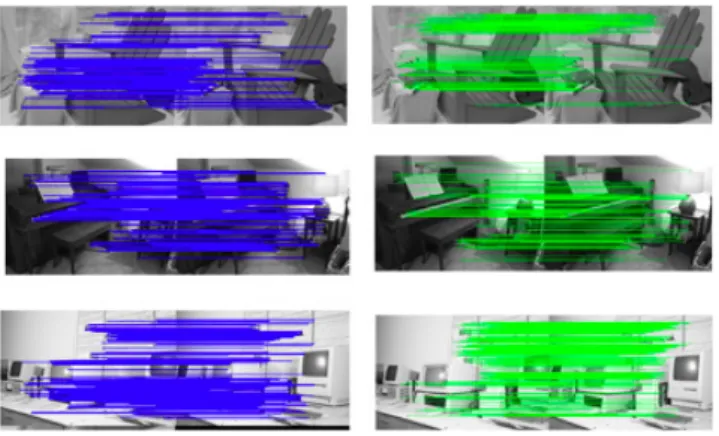
“Pipes”, accuracy of our methods is much higher than that of AKAZE. The true matching pairs obtained by our method, and AKAZE are shown in Fig. 7. The true matching pairs on the edges are obtained accurately by AKAZE, for example, the feature points on the keyboard of “Piano” and the book of “Adirondack”. On the other hand, the true matching pairs in the textured region are obtained accurately by our method, for example, the feature points on the map of

“Adirondack”, the floor of “Piano”, and the characters of

“Vintage”. From these results, our method is better for images with textured regions than AKAZE.

Fig. 7 The true matching pairs by AKAZE in blue lines, and by our method in green lines. The top one is for “Adirondack”, the middle one is for “Piano”, and the bottom one is for “Vintage”.

6. Conclusion

In this paper, we described a memory saving feature descriptor we propose. Our feature descriptor is calculated by comparing pixel values in the normalized patch around the feature point. The normalized patch is made scale invariant and rotation invariant by utilizing the calculation of the scale and the orientation of the feature point in the Scale-Invariant Feature Transform (SIFT) descriptor[1].

In experiments, we compared the results obtained with our descriptor with those obtained with ORB, BRISK and AKAZE. We found that when the feature vector size was small, our descriptor’s accuracy was better than that of ORB and BRISK and comparable with that of AKAZE for all cases. For the images with small textures, our descriptor’s accuracy was better than that of AKAZE. This means that our descriptor may be useful for portable devices with smaller memory size than PCs.

Subjects for future work will include examining ways to estimate the scale and orientation of the feature point.

Acknowledgments

This work was supported by JSPS KAKENHI Grant Num- bers 15X00445 and SCAT foundation.

References

[1] D.G. Lowe, “Distinctive image features from scale-invariant keypoints,” International Journal of Computer Vision, vol.60, no.2, pp.91–110, 2004.

[2] H. Bay, A. Ess, T. Tuytelaars, and L.V. Gool, “SURF: Speeded- up robust features,” Computer Vision and Image Understanding, vol.110, no.3, pp.346–359, 2008.

[3] V. Lepetit, P. Lagger, and P. Fua, “Randomized trees for real-time keypoint recognition,” Proc. IEEE Conference on Computer Vision and Pattern Recognition (CVPR ’05), vol.2, pp.775–781, 2005.

[4] M. Ozuysal, M. Calonder, V. Lepetit, and P. Fua, “Fast keypoint recognition using random ferns,” IEEE Trans. Pattern Anal. Mach.

Intell., vol.32, no.3, pp.448–461, 2010.

[5] M. Calonder, V. Lepetit, C. Strecha, and P. Fua, “BRIEF: Binary robust independent elementary features,” Proc. European Conference

(5)

on Computer Vision (ECCV ’10), vol.IV, pp.778–792, 2010.

[6] S. Leutenegger, M. Chli, and R. Siegwart, “BRISK: Binary robust invariant scalable keypoints,” Proc. IEEE International Conference on Computer Vision (ICCV ’11), pp.2548–2555, 2011

[7] E. Rosten, R. Porter, and T. Drummond, “Faster and better: A ma- chine learning approach to corner detection,” IEEE Trans. Pattern Anal. Mach. Intell., vol.32, no.1, pp.105–119, 2010.

[8] E. Rublee, V. Rabaud, K. Konolige, and G. Bradski, “ORB: An ef- ficient alternative to SIFT or SURF,” Proc. IEEE Intetnational Con- ference on Computer Vision (ICCV ’11), pp.2564–2571, 2011.

[9] P. Alcantarilla, J. Nuevo, and A. Bartoli, “Fast explicit diﬀusion for accelerated features in nonlinear scale spaces,” Proc. British Ma- chine Vision Conference (BMVC ’13), pp.13.1–13.11, 2013.

[10] http://www.cs.ubc.ca/˜lowe/keypoints/

[11] http://vision.middlebury.edu/stereo/data/scenes2014/