INVITED PAPER
Special Section on Image Media QualityRecent Advances in Video Action Recognition with 3D Convolutions
Kensho HARA†a),Member
SUMMARY The performance of video action recognition has im- proved significantly in recent decades. Current recognition approaches mainly utilize convolutional neural networks to acquire video feature rep- resentations. In addition to the spatial information of video frames, tem- poral information such as motions and changes is important for recogniz- ing videos. Therefore, the use of convolutions in a spatiotemporal three- dimensional (3D) space for representing spatiotemporal features has gar- nered significant attention. Herein, we introduce recent advances in 3D convolutions for video action recognition.
key words: video recognition, action recognition, 3D convolutions, survey
1. Introduction
The use of deep convolutional neural networks (CNNs) in the field of computer vision has expanded significantly in recent years. ImageNet[1], which includes more than a mil- lion images, and other large-scale image datasets have con- tributed substantially to the creation of successful vision- based algorithms because the use of large-scale datasets is extremely important when using deep CNNs, which involve a large number of parameters. In addition to such large-scale datasets, a large number of algorithms, such as those for batch normalization[2]and residual learning[3], have been used to improve image classification performance. Feature representations acquired using very deep CNNs trained on large-scale datasets offer high generalization performance.
Using such a feature representation, can significantly im- prove the performance of several other tasks, including ob- ject detection [4], segmentation [5], and image caption- ing[6].
The performance of video action recognition, which is a task to recognize human actions in videos, has improved significantly by the development of deep CNNs for videos.
Similar to image recognition, CNNs with two-dimensional (2D) convolutions pretrained on ImageNet were initially used. A two-stream architecture, which is a popular ap- proach for CNN-based action recognition[7], uses RGB and stacked optical flow frames as appearance and motion in- formation, respectively; it demonstrates that combining two streams improves action recognition accuracy. Numerous methods based on two-stream CNNs have been proposed to achieve further improvements by introducing the advantage
Manuscript received June 30, 2020.
Manuscript revised October 18, 2020.
Manuscript publicized December 7, 2020.
†The author is with the National Instutite of Advanced Indus- trial Science and Technology, Tsukuba-shi, 305-8560 Japan.
a) E-mail: [email protected] DOI: 10.1587/transfun.2020IMP0012
of handcrafted features[8], different combining methods of two streams[9]–[11], and modeling of long-range temporal structures[12]. Wang et al. attempted to achieve good prac- tice for the training of very deep two-stream 2D CNNs[13].
Recently, CNNs with spatio–temporal three- dimensional (3D) convolutional CNNs (3D CNNs) have been shown to be more effective than CNNs with 2D kernels in action recognition [14]. Although 3D CNNs have been investigated for action recognition several years ago [15], they do not exhibit the advantages of two-stream 2D-based CNNs [16]. This is primarily due to the relatively small data scale of video datasets that are available for optimizing the immense number of parameters in 3D CNNs, which are much larger than those of 2D CNNs. In addition, 3D CNNs can only be trained on video datasets, whereas 2D CNNs can be pretrained on ImageNet. Recently, however, Car- reira and Zisserman achieved a significant breakthrough us- ing the Kinetics dataset, which includes large-scale videos.
They also introduced an inflation of 2D kernels pretrained on ImageNet into 3D ones [14]. Following these studies, 3D convolutions are mainly adopted in action recognition methods.
Herein, we introduce recent advances in 3D convolu- tions for video action recognition. Action recognition ap- proaches by handcrafted methods and early methods of deep learning have been summarized by Aggarwal and Ryoo[17]
and Herath et al.[18]. In contrast to these surveys, we focus on 3D convolutions herein. Section 2 explains the basics of 2D and 3D convolutions for action recognition, whereas Sect. 3 describes various network architectures with 3D con- volutions. We explain various state-of-the-art advances in Sect. 4 and introduce video datasets for training and evalu- ation in action recognition in Sect. 5. Finally, Sect. 6 con- cludes this paper.
2. Convolutions for Video Action Recognition
We explain the convolutions used for video action recog- nition. As described in the previous section, many studies utilized 2D convolutions for videos a few years ago, sim- ilar to image recognition. Recently, 3D convolutions have been mainly used in action recognition tasks because of the release of large-scale video datasets. Furthermore, (2+1)D convolutions, which are extended versions of 3D convolu- tions, contributed to high recognition performances. Fig- ure 1 shows an overview of the convolutions. In the follow- ing paragraphs, we introduce each convolution.
Copyright c2021 The Institute of Electronics, Information and Communication Engineers
Fig. 1 Convolutions for video action recognition. W,H, andTare width, height, and number of frames of the feature maps, respectively. 2D and 3D convolutions apply 1×Ks×KsandKt×Ks×Ks convolutional kernels, respectively. (2+1)D convolutions apply a 1×Ks×Kskernel at first, and then apply aKt×1×1 kernel separately. Note that this figure does not show the number of feature maps.
When applying a 2DKs×Ksconvolutional kernel into a video, i.e., a spatiotemporal 3D feature map, we applied it for each frame separately. This process is equivalent to directly applying a 1×Ks×Kskernel to a 3D feature map, as shown in Fig. 1(a). When applying 1×Ks×Ksconvolutional kernels with N channels into a T ×H×W input feature map withMchannels, the computational cost and number of parameters areT HW MK2sNandMKs2N, respectively. Some studies utilized a video as a feature map with 3 (RGB)×T (the number of frames) channels[7],[8],[13].
The size of a 3D convolutional kernel in the time di- mension differs from that of a 2D one, as shown in Fig. 1(b).
When applyingKt×Ks×Ksconvolutional kernels withN channels into aT×H×W input feature map withMchan- nels, the computational cost and number of parameters are T HW MK2sKtNandMKs2KtN, respectively. Compared with 2D convolutions, the computational cost and number of pa- rameters are increased byKt.
A (2+1)D convolution is a pseudo 3D convolution and comprises a spatial 2D convolution and a temporal 1D convolution, as shown in Fig. 1(c). The separated convo- lutions reduce the computational cost and number of pa- rameters while facilitating the training of deep neural net- works. When applying 1 × Ks × Ks and Kt × 1 × 1 convolutional kernels with Ns and Nt channels, respec- tively, into aT ×H×W input feature map with M chan- nels, the computational cost and number of parameters are
T HW MK2sNs+T HW NsKtNt = T HW(MK2sNs+NsKtNt) and MK2sNs +NsKtNt, respectively. When Nt = N and Ns=(MK2sKtN)/(MKs2+NKt), the computational cost and number of parameters are the same as those of 3D convo- lutions. Tran et al. demonstrated that (2+1)D convolutions outperformed 3D convolutions in action recognition when the number of parameters of (2+1)D convolutions was the same as that of 3D convolutions[19].
3. Network Architectures with 3D Convolutions In this section, we introduce 3D CNN architectures for ac- tion recognition. In the tables presented, the input sizes of the network architectures listed are based on original publi- cations.
3.1 C3D
C3D proposed by Tran et al.[20]is a popular 3D CNN ar- chitecture. Table 1 shows the network architecture of C3D.
The architecture of C3D is based on VGG-11[21]proposed for image classification; 2D convolutions with 3×3 ker- nels in VGG-11 are replaced with 3D convolutions with 3×3×3 kernels in C3D. All activation functions of C3D are ReLU[22]. The best kernel temporal depth demonstrated by Tran et al. was three. This value has been used in subsequent architectures.
Table 1 Network architecture of C3D.Cis the number of classes.conv, maxpool, andfcare the convolutional, max pooling, and fully connected layers, respectively.
Layer Output Size Kernel size Stride input 3×16×112×112
conv 64×16×112×112 3×3×3 1, 1, 1 maxpool 64×16×56×56 1×2×2 1, 2, 2 conv 128×16×56×56 3×3×3 1, 1, 1 maxpool 128×8×28×28 2×2×2 2, 2, 2 conv×2 256×8×28×28 3×3×3 1, 1, 1 maxpool 256×4×14×14 2×2×2 2, 2, 2 conv×2 512×4×14×14 3×3×3 1, 1, 1 maxpool 512×2×7×7 2×2×2 2, 2, 2 conv×2 512×2×7×7 3×3×3 1, 1, 1 maxpool 512×1×4×4 2×2×2 2, 2, 2
fc 4096
fc 4096
fc C
C3D is expected to yield spatio–temporal feature rep- resentations because it utilizes spatio–temporal 3D convo- lutions. However, similar to 2D CNNs, the two-stream en- sembling of RGB frames and stacked optical flows improve the recognition performance of C3D[16]. Such results have been reported in other 3D architectures[14],[19],[23]as well.
3.2 I3D
An inflated 3D CNN (I3D)[14]is a 3D convolutional net- work architecture based on GoogLeNet (inception-v1)[24].
Table 2 shows the architecture of an I3D, and Fig. 2 shows the inception module, which is proposed to efficiently com- pute wider and deeper networks in GoogLeNet. The output of an I3D based on a video clip includes the class proba- bilities of multiple frames. The average probability of the frames should be calculated to acquire the class probabili- ties of the video clip.
An important point in an I3D is inflation, i.e., the con- version of successful 2D classification models into 3D ones.
The inflation operation repeats the weights of 2D kernelsN times along the time dimension and rescales them by divid- ing byN. Carreira and Zisserman demonstrated that the 3D inflated models of 2D GoogLeNet pretrained on ImageNet achieved better performances compared with non-inflated models[14].
One of the techniques to extend 2D GoogLeNet to 3D I3D is by configuring the kernel temporal depths and strides of the max pooling layers. The depths and strides of the first and second max pooling layers are not three, which is the value of the spatial dimensions, but one. Carreira and Zis- serman described that they configured the depths and strides to grow the receptive field gradually in time and to avoid conflating edges from different objects, which can hinder early feature detection[14].
Table 2 Network Architecture of I3D.Cis the number of classes;conv, maxpool, andavgpooldenote the convolutional, max pooling, and average pooling layers, respectively. Inceptionindicates the inception module, as shown in Fig. 2.
Layer Output Size Kernel size Stride
input 3×64×224×224
conv 64×32×112×112 7×7×7 2, 2, 2 maxpool 64×32×56×56 1×3×3 1, 2, 2 conv 64×32×56×56 1×1×1 1, 1, 1 conv 192×32×56×56 3×3×3 1, 1, 1 maxpool 192×32×28×28 1×3×3 1, 2, 2 inception×2 480×32×28×28
maxpool 480×16×14×14 3×3×3 2, 2, 2 inception×5 832×16×14×14
maxpool 832×8×7×7 3×3×3 2, 2, 2 inception×2 1024×8×7×7
avgpool 1024×8×1×1 2×7×7 1, 1, 1
conv C×8 1, 1, 1 1, 1, 1
Fig. 2 3D inception module. This 3D inception module replaces the 5×5 convolutional layer of the 2D inception module[24]with not a 5×5×5 layer but a 3×3×3 layer.
Fig. 3 3D bottleneck residual module.
3.3 3D ResNet
3D ResNet[25]–[27], also known as R3D[19], is a 3D ver- sion of the 2D residual network (ResNet)[3]. ResNet pro- vides shortcut connections that allow a signal to bypass one layer and move to the next layer in a sequence, as shown in Fig. 3. Because these connections pass through the net- work’s gradient flows from the latter layers to the early lay- ers, they can facilitate the training of very deep networks.
Table 3 shows the architecture of 3D ResNet-50.
The recognition performances of deeper 3D ResNets trained on a large-scale video dataset, such as Kinetics[28],
Table 3 Network Architecture of 3D ResNet-50. Cis the number of classes;conv,maxpool, avgpool, andfcdenote the convolutional, max pooling, average pooling, and fully connected layers, respectively.Resid- ualindicates the residual module shown in Fig. 3.
Layer Output Size Kernel size Stride
input 3×16×112×112
conv 64×16×56×56 7×7×7 1, 2, 2
maxpool 64×8×28×28 3×3×3 2, 2, 2
residual×3 256×8×28×28
1×1×1,64 3×3×3,64 1×1×1,256
1, 1, 1
residual×4 512×4×14×14
1×1×1,128 3×3×3,128 1×1×1,512
2, 2, 2
residual×6 1024×2×7×7
1×1×1,256 3×3×3,256 1×1×1,1024
2, 2, 2
residual×3 2048×1×4×4
1×1×1,512 3×3×3,512 1×1×1,2048
2, 2, 2
avgpool 2048×1×1×1 1×7×7 1, 1, 1
fc C
are better than those of shallower models, similar to the im- age recognition performance of 2D ResNets[3]. Hara et al.
demonstrated that improvements using deeper models con- tinued until a depth of 152 was reached[26]. Extended ver- sions of ResNets, such as pre-activation ResNet[29], wide ResNet[30], and ResNeXt[31], have also been investigated, in which ResNeXt-101 achieved the best performance[26].
3.4 P3D, R(2+1)D, and S3D
P3D[32], R(2+1)D[19], and S3D[23]utilize pseudo 3D convolutions; currently, they are often known as (2+1)D convolutions, as described in Sect. 2. (2+1)D convolutions apply spatial 2D convolutions, followed by temporal 1D convolutions. The same idea has been introduced in fac- torized spatio–temporal convolutional networks[33]. The network architectures of P3D and R(2+1)D are based on the 3D ResNet, and S3D is an I3D-based architecture. These models replace 3D convolutions with (2+1)D convolutions.
P3D introduces different designs of the pseudo 3D con- volutions. P3D-A adopts the same design as (2+1)D convo- lutions.
y= ft(fs(x)), (1)
wherexandyare the input and output of the convolution; fs
and ft are functions that apply 2D spatial and 1D temporal convolutions, respectively. P3D-B applies both spatial 2D and temporal 1D kernels in different pathways in a parallel manner and then accumulates both pathways into the final output.
y= fs(x)+ft(x). (2)
Fig. 4 Non-local module.
P3D-C utilizes a design combining those of P3D-A and P3D-B.
y= ft(fs(x))+fs(x). (3) All designs are used with skip connections, similar to the residual module in P3D. Qiu et al. demonstrated that com- bining the three designs in the network yielded the best per- formance[32].
Xie et al. investigated top-heavy and bottom-heavy S3Ds, which utilize (2+1)D convolutions in some layers and 2D convolutions in the remaining ones[23]. They demon- strated that a model that maintained the top two layers as (2+1)D convolutions, and the remaining as 2D convolu- tions yielded a good speed-accuracy tradeoff, and that using (2+1)D convolutions in all layers yielded the best accuracy.
Furthermore, they also proposed S3D-G, which introduces a self-attention mechanism after each temporal convolutions in S3D. Its attention mechanism improved the recognition performance.
3.5 Non-Local Neural Networks
Non-local neural networks utilize non-local operations to capture long-term dependencies of actions [34]. Non-local operations compute the response at a position as a weighted sum of the features at all positions in the input feature maps, as shown in Fig. 4.
yi= 1 P
∀j f(xi,xj) X
∀j
f(xi,xj)g(xj), (4) f(xi,xj)=eθ(xi)φ(xj), (5) whereiis the index of an output spatio-temporal position; j is the index that enumerates all possible positions;g, θ,and φare embedded representations. Because the operation con- siders all spatio-temporal positions, the operation can cap- ture long-term dependencies, which are difficult to capture by convolutions.
Wang et al. used 3D ResNet-50 based non-local net- work architectures [34], where non-local blocks were in- serted into the third and fourth residual blocks of the 3D ResNet-50. They discovered that the non-local 3D ResNet- 50 achieved better performances than 3D ResNet-101 with-
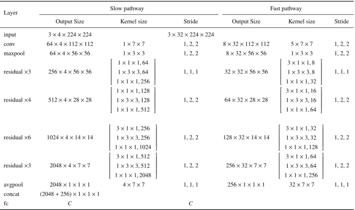
Table 4 Network Architecture of SlowFast 3D ResNet-50.Cis the number of classes.conv,max- pool,avgpool, andfcmean convolutional, max pooling, average pooling, and fully-connected layers, respectively.concatconcatenates the outputs of slow and fast pathways.
Layer Slow pathway Fast pathway
Output Size Kernel size Stride Output Size Kernel size Stride
input 3×4×224×224 3×32×224×224
conv 64×4×112×112 1×7×7 1, 2, 2 8×32×112×112 5×7×7 1, 2, 2
maxpool 64×4×56×56 1×3×3 1, 2, 2 8×32×56×56 1×3×3 1, 2, 2
residual×3 256×4×56×56
1×1×1,64 1×3×3,64 1×1×1,256
1, 1, 1 32×32×56×56
3×1×1,8 1×3×3,8 1×1×1,32
1, 1, 1
residual×4 512×4×28×28
1×1×1,128 1×3×3,128 1×1×1,512
1, 2, 2 64×32×28×28
3×1×1,16 1×3×3,16 1×1×1,64
1, 2, 2
residual×6 1024×4×14×14
3×1×1,256 1×3×3,256 1×1×1,1024
1, 2, 2 128×32×14×14
3×1×1,32 1×3×3,32 1×1×1,128
1, 2, 2
residual×3 2048×4×7×7
3×1×1,512 1×3×3,512 1×1×1,2048
1, 2, 2 256×32×7×7
3×1×1,64 1×3×3,64 1×1×1,256
1, 2, 2
avgpool 2048×1×1×1 4×7×7 1, 1, 1 256×1×1×1 32×7×7 1, 1, 1
concat (2048+256)×1×1×1
fc C C
out non-local blocks, even though the numbers of parame- ters and layers of the non-local 3D ResNet-50 were smaller.
3.6 SlowFast Networks
SlowFast networks[35]comprises two pathways that are de- signed based on biological studies. One pathway, known as the slow pathway, captures spatial semantics at a low frame rate, whereas the other one, known as the fast pathway, cap- tures motion at a fine temporal resolution. Table 4 shows the architecture of the SlowFast network. The temporal sizes of the inputs of both pathways are based on the frame rate of the input video instead of its duration. The network only uti- lizes pure 3D convolutions in the first convolution of the fast pathway. The other convolutions are 2D spatial or 1D tem- poral convolutions. The slow pathway uses temporal convo- lutions only in the third and fourth residual blocks because using temporal convolutions in the early layers degrades the accuracy[35]. The fast pathway has a smaller number of feature maps compared with the slow pathway for an effi- cient computation. Such a thinner architecture of the fast pathway degrades the performance only slightly. The frame rates of the slow and fast pathways used are 1/16 and 1/2 of the original videos, respectively. The SlowFast network in- cludes lateral connections between the two pathways to fuse information, similar to two-stream architectures[9]–[11].
3.7 X3D
X3D is an efficient network architecture for video action recognition[36]. The architecture is based on a 2D ResNet structure and the Fast pathway design of SlowFast networks.
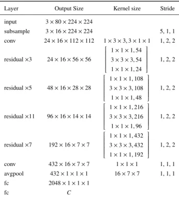
Feichtenhofer discovered the most efficient architecture by progressively expanding a small base 2D architecture across the following axes: temporal duration, frame rate, spatial resolution, network width, bottleneck width, and depth. One of the architectures, known as X3D-M, is shown in Ta- ble 5. X3D-M is expanded across the bottleneck width, temporal resolution, spatial resolution, depth, temporal du- ration, temporal resolution, temporal duration, and spatial resolution, in that order. These progressive expansions in- dicate that networks with thin channel dimensions and high spatiotemporal resolution can be effective for video action recognition. Larger X3D-XL achieved performances simi- lar to those of a method combining SlowFast and non-local networks whereas the combined method requires 4.8 times larger multiply–add computations compared with the X3D- XL. The performance of X3D-M is slightly worse than that of X3D-XL although its multiply–add computations are 7.8 times fewer.
3.8 Summary
As above-mentioned, various 3D CNN architectures have been proposed. ResNets, described in Sect. 3.3, were often
Table 5 Network Architecture of X3D-M.Cis the number of classes;
conv,avgpool, andfcdenote the convolutional, average pooling, and fully connected layers, respectively.Subsamplesubsamples the input videos in the time dimension.
Layer Output Size Kernel size Stride
input 3×80×224×224
subsample 3×16×224×224 5, 1, 1
conv 24×16×112×112 1×3×3,3×1×1 1, 2, 2
residual×3 24×16×56×56
1×1×1,54 3×3×3,54 1×1×1,24
1, 2, 2
residual×5 48×16×28×28
1×1×1,108 3×3×3,108 1×1×1,48
1, 2, 2
residual×11 96×16×14×14
1×1×1,216 3×3×3,216 1×1×1,96
1, 2, 2
residual×7 192×16×7×7
1×1×1,432 3×3×3,432 1×1×1,192
1, 2, 2
conv 432×16×7×7 1×1×1 1, 1, 1
avgpool 432×1×1×1 16×7×7 1, 1, 1
fc 2048×1×1×1
fc C
used in recent studies as a backbone architecture because they contains various depth configurations, such as ResNet- 18, -34, -50, -101, -152, and -200. We can select the depth configuration based on speed-accuracy tradeoff. Instead of 3D convolutions, (2+1)D convolutions (i.e. R(2+1)D), de- scribed in Sect. 3.4, were also often used and improved the recognition accuracy whereas using (2+1)D convolutions sometimes increases memory requirements in the training steps as the number of layers increases by two times (2D and 1D convolutions). Adding non-local operations, SlowFast pathways, and optical flow stream helps further improve- ments of the recognition accuracy.
4. Analyses and Improvements of 3D CNNs
4.1 Analyses of 3D CNNs
3D CNNs are analyzed from various aspects. We classify some analyses and explain them in this section.
4.1.1 Input Sizes
Varol et al. analyzed the temporal duration of the input to 3D CNNs[16]. They indicated that the temporal duration of C3D (= 16 frames) was insufficient to capture spatio–
temporal structures of the actions. They investigated the ef- fect of the temporal duration on the recognition accuracy by varying the durations. Their results indicated that longer durations resulted in higher accuracies. Similar results have also been reported in[26],[34],[36].
In addition to the temporal duration, spatial and tempo- ral resolutions affect the recognition performance. Higher spatio–temporal resolutions yielded higher recognition ac- curacies, and the contribution was significant, as described in Sect. 3.7. However, a tradeoff exists between recogni- tion accuracy and computational costs. A study has been conducted to improve the tradeoffin training, which will be described later in Sect. 4.3.
4.1.2 Motion Information
Ensembling with RGB frames (appearance) and optical flows (motion) improves recognition performance even when using 3D CNNs[14],[16],[19], which can theoret- ically acquire spatio–temporal representations. This indi- cates that 3D CNNs cannot utilize motion information when classifying videos. In this regard, Huang et al. tested a model trained with full-length videos on a single subsam- pled frame (i.e., without motion information) [37]. How- ever, they observed that subsampling resulted in a distri- bution shift in the temporal dimension, and that subsam- pling occasionally removed important frames for recogniz- ing the action. To avoid artifacts, they proposed two meth- ods that compensate for the distribution gap and selected the appropriate frames without including any motion informa- tion. Their experimental results indicated that when using their proposed methods, the recognition accuracy decreased by only 5% from the 47% accuracy on the Kinetics dataset when evaluating tighter upper bounds without motion infor- mation. It is considered likely that their result also indicates that 3D CNNs did not focus on motion information in clas- sification of the videos of Kinetics. Motivated by these re- sults, some studies have been conducted to improve motion representation of 3D CNNs, as described in Sect. 4.2.
4.1.3 Training Data
The scale of training data is important for training 3D CNNs. Kay et al. demonstrated that C3D achieved slightly better performances compared with 2D ResNet-50 when the model was trained on a large-scale Kinetics dataset, al- though the accuracy of C3D trained on the relatively small UCF-101 dataset was low[28]. Kataoka et al. compared the performance of models pretrained on various datasets[38], such as Kinetics-700[39]and Moments in Time[40]. Their results indicated that Kinetics-700 pretrained on 3D ResNet- 50 achieved the best performance compared with the model pretrained on the other datasets. In addition, to increase the amount of training data using public datasets, they concate- nated the Kinetics-700 and Moments in Time datasets from 650K videos/700 and 1M videos/339 categories, respec- tively, into 1.65M videos/1,039 categories and pretrained 3D ResNet-50 on the concatenated dataset. Their experiment demonstrated that pretraining on the concatenated dataset further improved the accuracy. Ghadiyaram et al. trained 3D CNNs on 65 million videos obtained from a social media website[41]. The video labels were annotated based on the
hash tags of videos, which often include noise. They demon- strated that pretraining on such large-scale videos with noisy labels significantly improved the recognition performance, and that the performance of R(2+1)D-34 improved log- linearly with training data size.
Data augmentation methods for 3D CNNs have been discussed as well. Hara et al. compared various strategies for cropping video clips[42]. Their results indicated that spatio–temporal crop positions should be selected randomly, and that the spatial scale of the cropping should be random but the temporal scale should be fixed.
4.2 Improvements in Motion Representation
Recently, studies have been conducted to improve motion representation. As described in Sect. 4.1.2, some problems are encountered in the motion representation of 3D CNNs.
One of the solutions is to use optical flows, but the compu- tational cost of calculating optical flows is high. Inspired by the TV-L1 algorithm[43], which is an optical flow esti- mation method, Piergiovanni et al. proposed a CNN layer to compute feature flows[44]. Their proposed representation flow layer unrolls the iteration computations of TV-L1 and implements similar computations as a differentiable layer with learnable parameters. Therefore, the representation flow layer can be optimized for action recognition. They applied their layer on lower-resolution feature maps for an efficient computation. Their experimental results showed that 3D and (2+1)D ResNet-18 with representation layers achieved higher accuracies than those without the layers. In- spired by the correlation layer of FlowNet[45], Wang et al.
proposed a correlation operator [46], which is similar to the representation flow. The correlation operator computes the correlations between every pair of adjacent frames in the feature maps. Motion information is acquired based on frame-wise correlations (i.e., similarities). The correlation operator is differentiable and implemented with learnable parameters. They inserted their correlation operators into the first, second, and third residual blocks of R(2+1)D-26.
Their network involving correlation operators and not re- quiring optical flows, known as CorrNet, achieved perfor- mances similar to those of two-stream backbone models.
Zhu et al. used optimized optical flows for action recog- nition by introducing a hidden two-stream architecture that included an optical flow estimation module[47].
Stroud et al. attempted another approach involving dis- tillation[48]. They trained a network that recognizes ac- tions using optical flows as a teacher network and distills knowledge from a teacher to a student network that uses RGB frames. Because optical flows are only used by the teacher network, which is only used in training, the infer- ence step is efficiently executed without computing flows.
Their proposed D3D yielded performances that were com- parable with the two-stream approach, without requiring an optical flow in inference. Similarly, ActionFlowNet in- volves multitask learning that optimizes action recognition and optical flow estimation simultaneously[49], instead of
distillation.
Several studies have been conducted to acquire motion information using 2D-based architectures[50]–[54].
4.3 Efficient Training/Inference
It is important to ensure efficient training and inference with 3D CNNs, which can achieve high performances while maintaining a low computational cost. Wu et al. pro- posed an efficient training method using variable mini-batch shapes with different spatio–temporal resolutions[67]. As described in Sect. 4.1.1, spatio–temporal resolutions (input sizes) relate to the tradeoffbetween computational costs and recognition accuracies. Training with larger resolutions im- proves recognition accuracies as well as increases the train- ing time. Their proposed method varies the resolutions from coarse to fine during training. Training SlowFast ResNet- 50 using their method slightly improved the accuracy and decreased the training time by 4.5 times. SCSampler, pro- posed by Korbar et al., reduced the computational cost of action recognition [68]. SCSampler samples a reduced set of salient clips from a video. Recognizing actions using only salient clips is extremely efficient. SCSampler effi- ciently samples salient clips by directly using compressed videos without MPEG-4 and H.264 decodings, similar to compressed action recognition[69]. Their experimental re- sults demonstrated that using SCSampler not only improved the accuracy, but also significantly reduced the computa- tional cost.
Another approach has been proposed that uses group convolutions [31]and depthwise convolutions[70], which are more efficient than standard convolutions.
Luo and Yuille proposed an architecture using group convo- lutions[71]. They decomposed a 3D 3×3×3,Fconvolution into 2D 1×3×3,(1−α)Fand 3D 3×3×3, αFbased on group convolutions. In addition to the efficient computation based on group convolutions, decomposition encourages the chan- nels in each group to concentrate on static semantic features and dynamic motion features separately, thereby affording an easier training. Their proposed method enabled an effi- cient action recognition without decreasing the recognition accuracy. Tran et al. introduced depthwise convolutions into a 3D ResNet[72]. They replaced the 3×3×3 convolution of a bottleneck block with a 1×1×1 traditional convolution and a 3×3×3 depthwise convolution. They demonstrated that using deeper architectures, such as those with 101 layers and combined with such depthwise convolutions, a slightly better performance was achieved compared with that of the traditional 3D ResNet, with three times fewer FLOPs.
5. Video Datasets
In this section, we introduce popular video datasets for ac- tion recognition. We summarize the statistics of the video datasets in Table 6. Although many video datasets exist for other video recognition tasks, such as spatio–temporal ac- tion detection[73], action segmentation[74], video caption-
Table 6 Statistics of video datasets for action recognition.Yearshows not released years of the cited publications but the actual years of releasing datasets.YouTube*in the row of Moments in Time means YouTube and other internet video sources, such as Flickr, Vine, and Vimeo.
Dataset Year Source
Trimmed/ Temporal annotations
Number of classes
Number of videos/instances
HMDB-51[55] 2011 Movies/YouTube Yes 51 6,766
UCF-101[56] 2012 YouTube Yes 101 13,320
Sports-1M[57] 2014 YouTube No 487 1,133,158
ActivityNet[58] 2015 YouTube Yes 200 28,108
Charades[59] 2016 Crowdsorcing Yes 157 66,500
YouTube-8M[60] 2016 YouTube No 4,800 8,264,650
Kinetics-400[28] 2017 YouTube Yes 400 306,245
Something-Something[61] 2017 Crowdsorcing Yes 174 108,499
Moments in Time[40] 2018 YouTube* Yes 339 1,000,000
STAIR-Actions[62] 2018 YouTube/Crowdsorcing Yes 100 109,478
Kinetics-600[63] 2018 YouTube Yes 600 495,547
Something-Something-v2[64] 2018 Crowdsorcing Yes 174 220,847
Kinetics-700[39] 2019 YouTube Yes 700 650,317
HACS Clips[65] 2019 YouTube Yes 200 1,500,000
HACS Segments[65] 2019 YouTube Yes 200 139,000
FineGym[66] 2020 YouTube Yes 530 32,697
ing[75], learning text-video embeddings[76], and under- standing human–object relationships[77], we only discuss datasets used for action recognition.
5.1 Trimmed Video Datasets
Most video datasets contain videos that are temporally trimmed to remove non-action frames. The duration of each video ranges from several seconds to approximately 10 s.
These datasets are used for action recognition, in which a video is used as an input and an action label is output.
UCF-101[56]and HMDB-51[55]are popular datasets for action recognition. Most videos are collected from YouTube except the videos from movies in HMDB-51.
These datasets were released as large-scale video datasets in 2011 and 2012, respectively, and are used as popular bench- mark datasets even in 2020. Nevertheless, studies that do not include the performances of the two datasets will in- crease gradually because the accuracies on the datasets were almost saturated.
Kinetics datasets are the most frequently used video datasets in 2020. Kinetics-400, which contains videos clas- sified into 400 action classes, was released in 2017[28];
subsequently, the dataset was extended to Kinetics-600 and -700 [39], [63], which have a higher number of classes.
The videos in these datasets were collected from YouTube and annotated by crowd workers. Because Kinetics datasets include hundreds of thousands of videos, which are suffi- cient for training deep 3D CNNs[26], Kinetics pretrained on CNNs are used as base models in various tasks. Similar to Kinetics, Moments in Time, which include a larger num-
ber of action instances and a smaller number of classes than Kinetics, has been released[40]. HACS Clips[65]consists of 1.5M annotated clips sampled from 504K untrimmed videos. Zhao et al. demonstrated that recognition mod- els pretrained on HACS Clips achieved better performances compared with the models pretrained on Kinetics-600, Mo- ments in Time, and Sports1M datasets [65]. FineGym fo- cuses on fine-grained action recognition in gymnastic videos and provides class labels in a three-level semantic hierarchy.
In addition to the datasets above, which were collected primarily from YouTube, datasets that include videos cap- tured by crowd workers exist as well. Whereas YouTube- based datasets comprise actions in various domains, most crowdsourced datasets focus on daily activities. STAIR- Actions [62] includes daily actions at home, whereas Something-Something comprises daily object manipula- tions. Because Something-Something [61], [64] includes action pairs, which are difficult to classify without tempo- ral information such aspull somethingandpush something, it is used in studies discussing temporal feature representa- tion[78],[79].
5.2 Untrimmed Video Datasets with Temporal Annota- tions
In addition to the datasets mentioned in the previous sec- tion, video datasets that contain untrimmed videos involv- ing multiple actions exist. Charades[59]is a video dataset collected by crowd workers and focuses on daily activities.
One video in the dataset includes approximately 6.8 actions on the average. Temporal annotations that indicate the start
and end positions in time for each action are annotated. Sim- ilar to Charades, ActivityNet[58]is an untrimmed YouTube video dataset in various domains. One video in Activi- tyNet includes approximately 1.4 actions on the average.
Recently, larger untrimmmed datset known as HACS Seg- ments, which contains 139K action segments densely anno- tated in 50K untrimmed videos spanning 200 action cate- gories, is released[65].
These datasets can be used not only for action recog- nition by trimming videos based on temporal annotations, but also for temporal action localization, which estimates begin and end positions in the time of actions, as well as for untrimmed action recognition, which classify actions in videos that include non-action frames.
5.3 Untrimmed Video Datasets with Video-Level Labels Instead of detailed annotations, large-scale video datasets with video-level labels have been released. Sports-1M[57]
includes one million videos in the sports domain. YouTube- 8M[60]includes eight million videos in various domains.
A video in both datasets has one/multiple labels without be- ginning and end positions in time.
Although few studies have used these datasets because they are extremely large to be utilized easily and include noisy labels, some studies have used these datasets as large- scale video data for training deep models[20],[80].
6. Conclusion
We introduced various 3D convolutional network architec- tures and presented their analyses and improvements in video action recognition. Video action recognition has de- veloped rapidly in recent years, whereas numerous methods and large-scale video datasets have been proposed. Mod- els and datasets become larger every year; consequently, the computational resources required for video research has in- creased. Meanwhile, efficient training and inference meth- ods have been developed recently (although some of them require significant resources to develop their algorithms).
Improving motion representation of 3D CNNs is also inter- esting topic. Future studies will be conducted to address these current shortcomings.
References
[1] J. Deng, W. Dong, R. Socher, L.J. Li, K. Li, and L. Fei-Fei, “Ima- geNet: A large-scale hierarchical image database,” Proc. IEEE Con- ference on Computer Vision and Pattern Recognition (CVPR), 2009.
[2] S. Ioffe and C. Szegedy, “Batch normalization: Accelerating deep network training by reducing internal covariate shift,” Proc. Interna- tional Conference on Machine Learning, pp.448–456, 2015.
[3] K. He, X. Zhang, S. Ren, and J. Sun, “Deep residual learning for image recognition,” Proc. IEEE Conference on Computer Vision and Pattern Recognition (CVPR), pp.770–778, 2016.
[4] S. Ren, K. He, R. Girshick, and J. Sun, “Faster R-CNN: Towards real-time object detection with region proposal networks,” Proc. Ad- vances in Neural Information Processing Systems (NIPS), pp.1–9, 2015.
[5] K. He, G. Gkioxari, P. Doll´ar, and R. Girshick, “Mask R- CNN,” Proc. International Conference on Computer Vision (ICCV), pp.2961–2969, 2017.
[6] K. Xu, J. Ba, R. Kiros, K. Cho, A. Courville, R. Salakhudinov, R. Zemel, and Y. Bengio, “Show, attend and tell: Neural image caption generation with visual attention,” Proc. International Con- ference on Machine Learning (ICML), pp.2048–2057, 2015.
[7] K. Simonyan and A. Zisserman, “Two-stream convolutional net- works for action recognition in videos,” Proc. Advances in Neural Information Processing Systems (NIPS), pp.568–576, 2014.
[8] L. Wang, Y. Qiao, and X. Tang, “Action recognition with trajectory- pooled deep-convolutional descriptors,” Proc. IEEE Conference on Computer Vision and Pattern Recognition (CVPR), pp.4305–4314, 2015.
[9] C. Feichtenhofer, A. Pinz, and R. Wildes, “Spatiotemporal residual networks for video action recognition,” Proc. Advances in Neural Information Processing Systems (NIPS), pp.3468–3476, 2016.
[10] C. Feichtenhofer, A. Pinz, and A. Zisserman, “Convolutional two- stream network fusion for video action recognition,” Proc. IEEE Conference on Computer Vision and Pattern Recognition (CVPR), pp.1933–1941, 2016.
[11] C. Feichtenhofer, A. Pinz, and R.P. Wildes, “Spatiotemporal multi- plier networks for video action recognition,” Proc. IEEE Conference on Computer Vision and Pattern Recognition (CVPR), 2017.
[12] L. Wang, Y. Xiong, Z. Wang, Y. Qiao, D. Lin, X. Tang, and L. Van Gool, “Temporal segment networks: Towards good practices for deep action recognition,” Proc. European Conference on Com- puter Vision (ECCV), pp.20–36, 2016.
[13] L. Wang, Y. Xiong, Z. Wang, and Y. Qiao, “Towards good practices for very deep two-stream convnets,” arXiv preprint, arXiv:1507.02159, 2015.
[14] J. Carreira and A. Zisserman, “Quo vadis, action recognition? A new model and the Kinetics dataset,” Proc. IEEE Conference on Computer Vision and Pattern Recognition (CVPR), pp.4724–4733, 2017.
[15] S. Ji, W. Xu, M. Yang, and K. Yu, “3D convolutional neural networks for human action recognition,” IEEE Trans. Pattern Anal. Mach. In- tell., vol.35, no.1, pp.221–231, 2013.
[16] G. Varol, I. Laptev, and C. Schmid, “Long-term temporal convolu- tions for action recognition,” IEEE Trans. Pattern Anal. Mach. In- tell., vol.40, no.6, pp.1510–1517, 2018.
[17] J. Aggarwal and M. Ryoo, “Human activity analysis: A review,”
ACM Comput. Surv., vol.43, no.3, 2011.
[18] S. Herath, M. Harandi, and F. Porikli, “Going deeper into action recognition: A survey,” Image and Vision Computing, vol.60, pp.4–
21, 2017.
[19] D. Tran, H. Wang, L. Torresani, J. Ray, Y. LeCun, and M. Paluri, “A closer look at spatiotemporal convolutions for action recognition,”
Proc. IEEE Conference on Computer Vision and Pattern Recogni- tion (CVPR), pp.6450–6459, 2018.
[20] D. Tran, L. Bourdev, R. Fergus, L. Torresani, and M. Paluri, “Learn- ing spatiotemporal features with 3D convolutional networks,” Proc.
International Conference on Computer Vision (ICCV), pp.4489–
4497, 2015.
[21] K. Simonyan and A. Zisserman, “Very deep convolutional networks for large-scale image recognition,” Proc. International Conference on Learning Representations (ICLR), pp.1–14, 2015.
[22] V. Nair and G.E. Hinton, “Rectified linear units improve restricted Boltzmann machines,” Proc. International Conference on Machine Learning, pp.807–814, Omnipress, 2010.
[23] S. Xie, C. Sun, J. Huang, Z. Tu, and K. Murphy, “Rethinking spa- tiotemporal feature learning: Speed-accuracy trade-offs in video classification,” Proc. European Conference on Computer Vision (ECCV), pp.318–335, 2018.
[24] C. Szegedy, W. Liu, Y. Jia, P. Sermanet, S. Reed, D. Anguelov, D. Er- han, V. Vanhoucke, and A. Rabinovich, “Going deeper with convo- lutions,” Proc. IEEE Conference on Computer Vision and Pattern