Application of deep learning in prediction of
cerebral white matter lesions using clinical
examination data
-
Optimization of prediction performance and
generalization performance and comparison with
conventional methods-
Hiroshi Yano (Kurume Univ.) Yuya Shinkawa (Kurume
Univ.) Kazuo Ishii (Kurume Univ.)
Abstract
Using medical examination data, mathematical modeling was applied on a clinical diagnosis to predict disease prognosis. With the assistance of a logistic regression model, we indicated earlier optimal mathematical modeling to predict cerebral white matter lesions (sensitivity 72.0% and specificity 75.1%) with 15 variables, including age, gender, systolic blood pressure, LDL cholesterol (LDL), and hemoglobin A1c (HbA1c), from brain dock examinees data (total 1904: 988 men and 916 women). In this account, the optimization of prediction and generalization performance by applying deep learning technology has resulted in the optimal predictive model (sensitivity 76.9% and specificity 74.4%) employing the logistic regression neural network model of a 64-node environment, dropout = 0.2 and L1 = 0.015. This model revealed some improvements, such as area under the curve (AUC) 0.809, accuracy 76.1%, and error rate 23.9%, compared with the previous record, and it was evidenced that deep learning could secure a more precise diagnostic prediction model through the medical examination data. Simultaneously, it was further shown that it is complicated and eventually impossible to interpret the prediction model by deep learning from the medical examination data compared with those by the linear prediction model based on causal reasoning.1. Introduction
The applications of deep learning (DL) in a clinical environment are increasing [1]. Specifically, DL has shown itself to be useful in diagnostic imaging [1] and promising in the application of natural language processing to real-world data, including electronic medical records and receipt data [2]. In addition, the diagnostic prediction of diseases through medical examination data has been reviewed by employing assorted mathematical models, and we additionally reported an optimal prediction model using a logistic regression model to predict cerebral white matter lesions with medical examination data (sensitivity 72.0% and specificity 75.1%) [3]. Despite this, although this model was maximized by model fitting through variable selection with the forward–backward stepwise selection approach, the generalization performance was not assessed, and consequently, the upgrade of the prediction performance was lacking.
optimized prediction model (sensitivity 76.9% and specificity 74.4%) employing the logistic regression model with a neural network under 64 node conditions, dropout = 0.2, and coefficient λ in L1 regularization (L1) = 0.015. This model displayed numerous improvements, such as area under the curve (AUC) 0.809, accuracy 76.1%, and error rate 23.9%, compared with the previous report, and it was demonstrated that DL could acquire a more exact diagnostic prediction model with the medical examination data. In contrast, with DL, it was further indicated that it is complicated to explanate clinical variables due to the difficulty acquiring coefficients based on causal inference. In this investigation, we communicate the betterment of the prediction performance of medical examination data by improving the generalization performance through DL and the complications of explanation clinical variables.
2. Materials and Methods
2.1 Subjects and ethical considerations
This research was performed employing data from 1,904 subject examinations, including 988 men and 916 women, who experienced head MRI and blood tests at the time of the brain dock course of a thorough medical examination at some point between April 1, 2016, and October 31, 2017, at the Shin Takeo Hospital, with the approval of the Ethics Committee of Shin Takeo Hospital and Kurume University. For patient privacy protection, the patient data were collected with connection-free anonymization by a third party and saved for research use only in a password-protected storage medium.
2.2 Clinical data
In this report, the following data were used, as illustrated in our prior research [3]. For the common examination, four attributes have been employed: age, gender, systolic blood pressure (SBP), and the presence of visceral steatosis (to ascertain metabolic syndrome). For blood and biochemical assessments, performed as a section of the complete medical analysis, two features were employed: LDL cholesterol (LDL) and hemoglobin A1c (HbA1c). For the ultrasonic trials, one property, carotid plaque score (PS) was applied. PS was computed as follows. The carotid artery was separated into four 15-mm-long portions: the central side of the common carotid artery (CCA), the peripheral side of the CCA, the bifurcation of the CCA, and the central side of the internal carotid artery. Then, the total of the peak values of intima–media thickness surpassing 1.1 mm was determined. In the inquiry into the specific health investigation, four questions, which were responded to by the participants when obtaining an exhaustive medical examination, were employed: concerning their experience with therapies to reduce blood pressure, medications to reduce blood sugar or insulin injection, treatments to decrease the cholesterol level of cholesterol or of neutral fat, as well as imbibing practice (regularly, occasionally, or scarcely drink [cannot drink]).
2.3 Analytical methods
2.3.1 Data preprocessing
In data modeling, age, gender, SBP, the establishment of metabolic syndrome, PS, LDL, HbA1c from clinical investigation data, background with treatments to reduce blood pressure, therapies to reduce blood sugar or insulin injection, remedies to decrease the level of cholesterol or of neutral fat, and consumption customs from the survey were applied as explanatory variables. The existence or deficiency of white matter lesions was used as the response variable. In the discrete variables, gender, the resolution of the metabolic syndrome, the experience with treatments to reduce blood pressure, the knowledge of pharmaceuticals to reduce blood sugar or insulin injection, the occasion with therapies to decrease the level of cholesterol or of neutral fat, and drinking habits were depicted into dummy variables. To resolve metabolic syndrome and drinking ways, which are not binary data, a dummy variable transformation by the One Hot approach [4] was implemented. The explanatory variables were normalized collectively with the continuous scale: age, PS, LDL, HbA1c, and SBP.
2.3.2 Model building with DL
The cross-entropy loss was employed as a loss function, and a method for stochastic optimization (Adam) [5] was used as the optimizer, and for the activation function, Rectified Linear Unit (ReLU) [6] was used in the intermediate layer, and the sigmoid function was implemented in the output layer. The model was enhanced by changing the conditions of the number of nodes, dropout rate [7], and L1 regularization [8].
2.3.3 Comparing the performance of DL
A 10-fold cross-validation was employed for comparing the achievement of DL. Accuracy, error rate, sensitivity, specificity, positive predictive value (PPV), and negative predictive value (NPV) were applied as assessment indices founded on median cross-entropy loss of ten times. In 10-fold cross-validation, following the division of the data into 10, machine learning was accomplished using one of the divided data as validation data and the rest as training data, and the process was repeated ten times without repeat usage of validation data, and then the median of the evaluation indexes was computed. In the receiver operating characteristic (ROC) curve, the sensitivity was charted to the vertical axis, the false positive rate (1-specificity) was charted to the horizontal axis for each threshold, and the AUC was determined. When the Youden index (sensitivity – (1 − specificity)) was maximized, the threshold value resolved the cutoff value [9].
2.3.4 Execution environment
Machine learning was accomplished by applying Google Colaboratory (Google Colab) with Python 3.6.8 and TensorFlow 1.15.0 as the back end from Keras 2.2.5 [10]. Each inspection for comparing operation was considered, implementing the following R package according to the previous research [3]. The subsequent software packages were applied: R
randomForest() function of the randomForest (ver4.6.14) for random forest (RF) [12]; and the NaiveBayes() function of the klaR (ver0.6.14) for Naive Bayes (NB) [13].
3. Results
3.1 Hyperparameter optimization of DL
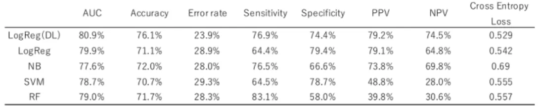
In the DL determination with medical examination data, 10-fold cross-validation gauged the prediction performance. Hyperparameters, including the number of nodes, dropout rate (dropout), and L1 were optimized by applying varied situations. The optimum prediction performance was acquired with an environment of 64 nodes, dropout = 0.2, and L1 = 0.015 (Figure 1). The vertical axis portrays the loss function (loss), and the horizontal axis depicts the number of epochs (epochs); the optimum learning model with a loss of approximately 0.53 was demonstrated at 100 epochs.
3.2 Comparing the performance of DL with different interpretive
approaches
Table 1 displays the outcomes of DL within the frame of node = 64, dropout = 0.2, and L1 = 0.015 and a parallel of different investigative approaches [3].
Figure 1. The optimum prediction performance under the conditions of 64 nodes, dropout = 0.2, and L1 = 0.015.
To compare the performance, a 10-fold cross-validation was executed and median values were determined. From top to bottom, logistic regression employing DL (LogReg (DL)), LogReg, NB, SVM, and RF have been illustrated.
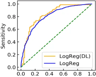
Consequently, LogReg (DL) exhibited the utmost performance in AUC (0.809), accuracy (76.1%), PPV (79.2%), and NPV (74.5%) and further afforded the least possible value of cross-entropy loss (0.529). Although it was subordinate to RF in sensitivity and LogReg and SVM in particularity, it was contemplated that the model with the premium generalization performance had been realized in the extensive view. The LogReg (DL) presented greater sensitivity and decreased specificity than LogReg. It is believed that LogReg (DL) displayed high sensitivity for the sake of attempting to expand the generalization ability and optimizing to augment the detection ability. Figure 2 illustrates the ROC curves of LogReg (DL) and LogReg.
3.3 Example of a model created in DL
An example of the model based on the node of the first layer for which the weight and bias were acquired in the model attained by conducting DL in the environment of 64 nodes, dropout = 0.2, and L1 = 0.015 is exhibited as follows. Because the quantity of nodes was actually 64, there are 64 models:
−0.014 − 0.000046𝑥(+0.00022𝑥+− 0.00015𝑥-− 0.00020𝑥.+ 0.00034𝑥0− 0.00012𝑥1 − 0.000045𝑥2+ 0.0000047𝑥4− 0.000034𝑥5+ 0.000047𝑥(6− 0.000021𝑥(( −0.000033𝑥(++ 0.00011𝑥(-− 0.00012𝑥(.+ 0.000044𝑥(0,
where 𝑥1 = age; 𝑥2 = gender (𝑥2 = 0 for male, and 𝑥2 = 1 for female); 𝑥3 = PS; 𝑥4 = LDL; 𝑥5 = SBP; 𝑥6 = HbA1c; 𝑥7 and 𝑥8 = the determination of metabolic syndrome; 𝑥7 = the
background with treatments to reduce blood pressure (x7 = 0 for “No,” x7 = 1 “Yes”); x8
= the knowledge of therapies to reduce blood sugar or insulin injection (x8 = 0 for “No,” x8
= 1 “Yes”); x9 = the understanding of pharmaceuticals to decrease the level of cholesterol
or of neutral fat (x9 = 0 for “No,” x9 = 1 “Yes”); x10, x11, and x12 = the specification of
syndrome); and x13, x14, and x15 = imbibing practices (x13 = 1, x14 = 0, and x15 = 0 for “rarely
drink (cannot drink)”; x13 = 0, x14 = 1, and x15 = 0 for “sometimes”; and 𝑥13 = 0, 𝑥14 =0, and 𝑥15 = 1 for “everyday”).
Following these nodes of the first layer, the classification is implemented in conformity with the output value in the output layer through the intermediate layer. Hence, such bias and value of the individual weight have various implications from the partial regression coefficient of the conventional regression model and may not be easily compared. In the preceding examination [3], the succeeding equation was achieved as a discriminant model:
log𝑃𝑟(𝑌?= 1| 𝑋?= 𝑥?)
𝑃𝑟(𝑌?= 0| 𝑋?= 𝑥?)= −0.28 + 1.1𝑥?(+ 0.45𝑥?++ 0.16𝑥?-+ 0.06𝑥F.+ 0.12𝑥?0 −0.04𝑥?1+ 0.43𝑥?2 + 0.15𝑥?4+ 0.42𝑥?5+ 0.37𝑥?(6+ 0.15𝑥?((+ 0.24𝑥?(++ 0.04𝑥?(-,
where the illustrative variables were identified as follows: x1 = age; x2 = gender (x2 = 0 for
male, x2 = 1 for female); x3 = PS; x4 = LDL; x5 = SBP; x6 = HbA1c; x7 and x8 = the assessment
of metabolic syndrome (x7 = 0 and x8 = 0 for non-metabolic syndrome; x7 = 1 and x8 = 0 for
the reserve of metabolic syndrome; and x7 = 1 and x8 = 1 for metabolic syndrome); x9 = the
awareness of medicinal products to reduce blood pressure (x9 = 0 for “No,” x9 = 1 for “Yes”);
x10 = the comprehension of medical care to reduce blood sugar or insulin injection (x10 = 0
for “No,” x10 = 1 for “Yes”); x11 = the perception of remedies to decrease the level of
cholesterol or of neutral fat (x11 = 0 for “No,” x11 = 1 for “Yes”); and x12 and x13 = the
imbibing customs (x12 = 0 and x13 = 0 for “rarely drink (cannot drink)”; x12 = 1 and x13 = 0
for “sometimes”; and x12 = 1 and x13 = 1 for “everyday”). For the i-th patient's data xi, Pr(Yi
= 1|Xi = xi) = the prospect that the i-th patient had the white matter lesions, and Pr(Yi = 0|Xi = xi) = the possibility that the i-th patient did not have white matter lesions.
The values of the particular coefficient of both weight and bias displayed a difference by three to four digits. The small value of the weight in DL is judged as the product of decreasing the weight by L1 regularization.
4. Discussions
In this analysis, we accomplished a machine learning model with increased generalization performance by logistic regression through DL compared with the previous investigation predicated on the medical examination data of 1,904 subjects who received head MRI and blood tests in the exhaustive medical inspection [3]. In DL, by hyperparameter optimization, comprising the number of nodes, dropout rate, and L1, the optimum state with the cross-entropy loss = 0.529 was procured under the circumstances of 64 nodes, dropout = 0.2, and L1 = 0.015. Adjusting the hyperparameters depicts a great impact on the model, and in this inquiry, trial and error was necessary because overfitting and scant knowledge were discovered subject to the setting context. In this inspection, by hyperparameter optimization completed by hand, the consideration of automatic optimization has been ongoing [14], which could deliver accelerated and more actual hyperparameter optimization. In this observation, DL displayed a more elevated sensitivity and declined specificity than that of logistic regression in the preceding study. This suggests that although the patient is negative,
a positive test conclusion can potentially occur, cerebral white matter lesions are perhaps to be presumed albeit the patient is normal comparing with the conventional approach. Moreover, it may be advantageous when the discovery of patients with assumed lesions from the total populace is requested instead of the unequivocal diagnosis.
Although conclusions were not revealed in this research, neither ridge regression (L2 regularization) [15] nor elastic net regression (L1–L2 regularization) [16] was feasible to secure a model with lower loss error and greater generalization performance than the lasso regression (L1 regularization) [8]. It was thought that because the model in this analysis had minimum 15 explanatory variables and the model is somewhat intricate, the consequence of the loss due to L2 regularization is less than that of L1 regularization. In other words, there is a compromise amid the bias and the variance component in regularization [16]. In a sophisticated model with small λ, the bias is apt to be small and the variance large, and within a high variance situation of that sort, the influence of suppressing overfitting by regularization is believed to be diminutive. Because the L2 regularization is more vulnerable to changes in λ than L1 regularization, it is regarded that the consequence of L2 regularization is reduced under such circumstances.
Typically, in machine learning, the connection between the response and explanatory variable is a black box, and just the discrimination outcome is output. In this analysis, we removed several nodes from the developed machine learning model and established their weights and biases. The findings did not mandatorily agree with traditional medical understanding, given the model is a blend of those nodes. Specifically, it was arduous to decipher the model. With respect to the clarification of DL models, it is feasible to compute the prominence or assistance employing software packages including LIME [17], SHAP [18], and Anchor [19] and to elucidate the involved black box models with strong intelligibility. Various approaches [20] have been put forward in which a problematic black box model is substituted by an extremely clear and explicable decision tree or a rule-based model. Nevertheless, they are incapable of expounding the true model adequately. Accordingly, it remains a continuing research to be determined.
5. Acknowledgments
This research was conducted as a research theme for the master's course of the Graduate School of Medicine, Kurume University. We would like to thank the faculty members, staff, graduate students, and other related participants for their cooperation and support. We would also like to thank Dr. Makoto Ichinose, Dr. Yohei Ohnaka, Dr. Takushi Yoshida, and hospital staff of Shin Takeo Hospital for their cooperation in providing valuable clinical data. We would like to thank Enago (www.enago.jp) for the English language review.
References
[1]. Cui S, Ming S, Lin Y, et al, Development and Clinical Application of Deep Learning Model for Lung Nodules Screening on CT Images. Sci Rep. 10(1):13657 (2020).
[3]. Shinkawa Y, Yoshida T, Onaka Y, Ichinose M, Ishii K, Mathematical modeling for the Prediction of Cerebral White Matter Lesions Based on Clinical Examination Data. PLoS ONE 14(4): e0215142 (2019).
[4]. David H, Sarah H, Digital Design and Computer architecture (2nd ed.). San Francisco, Calif.: Morgan Kaufmann. p. 129. ISBN 978-0-12-394424-5 (2012).
[5]. Kingma D, Adam BJ: A Method for Stochastic Optimization, 3rd International Conference for Learning Representations (ICLR 2015), San Diego. arXiv:1412.6980 (2015).
[6]. Agarap AF, Deep Learning using Rectified Linear Units (ReLU), Neural and Evolutionary Computing (cs.NE), arXiv:1803.08375 (2018).
[7]. Srivastava N, Hinton G, Krizhevsky A, Sutskever I, Salakhutdinov R, Dropout: A Simple Way to Prevent Neural Networks from Overfitting, J. Mach. Learn. Res. 15(56):1929-1958 (2014). [8]. Robert T, Regression Shrinkage and Selection via the Lasso. J. Royal Stat. Soc. B 58(1):267-288
(2014).
[9]. Ruopp MD, Perkins NJ, Whitcomb BW, Schisterman EF, Youden Index and Optimal Cut-Point Estimated from Observations Affected by a Lower Limit of Detection. Biomed. J. 50(3):419-430 (2008).
[10]. Abadi, M, Barham P, Chen J, et al, Tensorflow: A System for Large-Scale Machine Learning. Proc. 12th USENIX Symposium on Operating Systems Design and Implementation (OSDI 16) p. 265– 83 (2016).
[11]. Cortes C Vapnik V, Support-Vector Networks. Mach. Learn. 20(3), 273-297 (1995).
[12]. Ho TK, Random Decision Forests, Proc. 3rd International Conference on Document Analysis and Recognition, Montreal, QC, 14–16 August 1995. IEEE 1, pp. 278-282 (1995).
[13]. John GH, Langley P, Estimating Continuous Distributions in Bayesian Classifiers, Proc. Eleventh Conference on Uncertainty in Artificial Intelligence (UAI1995), UAI-P-1995-PG-338-345, arXiv:1302.4964 (1995).
[14]. Bergstra J, Yoshua B. Random Search for Hyper-Parameter Optimization. J. Mach. Learn. Res. 13:281-305 (2012).
[15]. Hoerl AE, Kennard RW, “Ridge Regression: Biased Estimation for Nonorthogonal Problems.” Technometrics 12(1):55-67 (1970).
[16]. Zou H; Hastie T, Regularization and Variable Selection via the Elastic Net. J. Royal Stat. Soc, B 67 (2):301-320 (2005).
[17]. Ribeiro MT, Singh S, Guestrin C, “Why should I trust you?”: Explaining the Predictions of Any Classifier, Proc. 22nd ACM SIGKDD International Conference on Knowledge Discovery and Data Mining-KDD '16. pp.1135-1144 (2005).
[18]. Lundberg S, Lee S-I, A Unified Approach to Interpreting Model Predictions, 31st Annual Conference on Neural Information Processing Systems (NIPS 2017), arXiv:1705.07874 (2017). [19]. Ribeiro MT,Singh S, C Guestrin C, Anchors: High-Precision Model-Agnostic Explanations, 32nd
AAAI Conference on Artificial Intelligence (2018).
[20]. Arrieta AB, Rodríguez ND, Ser JD, et al., Explainable Artificial Intelligence (XAI): Concepts, Taxonomies, Opportunities and Challenges toward Responsible AI, Inform. Fus. 58:82–115 (2020).
Hiroshi Yano(Regular member)[email protected]
Kurume University Graduate School of Medicine Master's course. Conducted biostatistics research focusing on the implementation of deep learning using medical examination data.
Yuya Shinkawa(Non-regular member)[email protected]
Kurume University Graduate School of Medicine Master's course. Conducted biostatistics research focusing on the optimization of mathematical modeling using medical examination data.
Kazuo Ishii(Regular member)[email protected]
Associate Professor, Center for Biostatistics, Kurume University. Completed the Graduate School of Medicine, Tokushima University, in 1995. Ph.D. (Medicine). Received the 2015 Information Processing Society of Japan Excellent Education Award. Engaged in big data analytics research in the medical and agriculture.
投稿受付:2020 年 11 月 30 日 採録決定:2020 年 12 月 4 日