Multifidelity modeling of deployable wings:
Multibody dynamic simulation and wind tunnel
experiment
著者
Keisuke Otsuka, Yinan Wang, Koji Fujita,
Hiroki Nagai, Kanjuro Makihara
journal or
publication title
AIAA journal
volume
57
number
10
page range
4300-4311
year
2019-01-01
URL
http://hdl.handle.net/10097/00130699
doi: 10.2514/1.J058676* Ph.D. Candidate, Department of Aerospace Engineering; [email protected]. † Postdoctoral Researcher, School of Engineering; [email protected]. ‡ Assistant Professor, Institute of Fluid Science; [email protected]. Member AIAA.
§ Professor, Institute of Fluid Science, Department of Aerospace Engineering; [email protected].
Senior Member AIAA.
¶ Professor, Department of Aerospace Engineering; [email protected]. Senior Member
AIAA.
Multifidelity Modeling of Deployable Wings:
Multibody Dynamic Simulation and Wind Tunnel
Experiment
Keisuke Otsuka*Tohoku University, Sendai 980-8579, Japan
Yinan Wang†
University of Warwick, Coventry, Warwickshire CV4 7AL, United Kingdom
Koji Fujita‡ and Hiroki Nagai§ Tohoku University, Sendai 980-8577, Japan
Kanjuro Makihara¶
2
Abstract
Slender deployable wings have attracted interest for use in Mars, Titan, and high-altitude flights. Such wings are composed of multiple bodies connected by hinge joints and can be deployed or folded spanwise during flight. A deployment simulation model is required for their design. This paper proposes a multifidelity multibody modeling method that utilizes a new asymmetrically gradient-deficient absolute nodal coordinate beam element. The proposed method addresses the drawbacks of conventional elements, namely, numerical locking and the need for a large number of generalized coordinates, by exploiting a structural characteristic of a slender wing. It enables computationally efficient low-fidelity rigid multibody simulation and more realistic high-fidelity flexible multibody simulation, both accomplished using a consistent modeling process and the same simulation program architecture. Additionally, the low-fidelity and high-fidelity models can be coupled with an aerodynamic model using a consistent coupling methodology. To validate the proposed modeling method, we performed wing deployment experiments in a wind tunnel at the Institute of Fluid Science, Tohoku University. The simulation results obtained using the proposed modeling method were found to be in good agreement with those of the wind tunnel experiments, even when the wings experienced large geometrically nonlinear deformations.
3
Nomenclature
A = cross-sectional area
A = aerodynamic influence coefficient matrix a = aerodynamic force vector
C = actuator damping
CL = lift coefficient
c = chord
E = Young’s modulus
EA, EIyy, EIzz = extensional and bending stiffnesses
e = generalized nodal coordinate vector
Fi = generalized force vector (i = actuator, aero, damping, gravity)
GJ = torsional stiffness
g = gravitational acceleration vector
h = beam thickness
Iyy, Izz = second moments of area
i, j, k = unit vectors for defining the element coordinate system
K = actuator stiffness
L = beam length
Lw = ratio between chord and considered wake length l = element length
n = vector normal to aerodynamic panel
Mconst = constant actuator torque
M = mass matrix
Δp = pressure difference between upper and lower surfaces of vortex panel
Qz = first moment of area
r = position vector of an arbitrary point rx, ry, rz = gradient vectors
4
S = shape matrixT, U = kinetic and elastic energies
Taero = maximum absolute value of aerodynamic torque acting around hinge axis Tconst = constant torque of spring actuator
U = uniform flow velocity ud = displacement vector
u, v, w = extensional and bending displacements
V = flow speed w = induced velocity
Δx, Δy = span- and chord-direction vortex panel lengths
o-xyz = element coordinate system
α = damping parameter Γ = circulation vector
Γ = circulation of vortex panel
εxx = extensional strain εyy, εzz = transverse strains κx = torsional curvature λ = Lagrange multiplier ρ = material density ρa = air density
Φ = constraint equation vector
ν = Poisson’s ratio
( )CP = value related to colocation point
( )Flexible = value related to flexible model
( )Rigid = value related to rigid model
( )VP = value related to vortex panel corner point
( )i = value related to node i (= A, B, C) ( )i,j = value related to bound vortex panel (i, j)
5
I. Introduction
IRCRAFT with slender deployable wings, an example of which is shown in Fig. 1a, have attracted attention in the aeronautical engineering community. Such wings are composed of multiple bodies connected by hinge joints and can be deployed or folded spanwise during flight. The deployable wings decrease the space required for storage of the aircraft and enable it utilization for diverse missions. Several deployable wing concepts have been developed for multiple-mission [1] and Mars [2, 3] aircraft since the turn of the 20th century. The wings usually have aspect ratios of <10, although some more recent concepts have larger aspect ratios. In 2018, Thai et al. [4] proposed a deployable wing concept with a 20.6 aspect ratio for use on an aircraft to explore Titan. Recent studies have also been conducted on the application of such slender deployable wings to aircraft powered by solar energy generated by solar panels mounted on the wings. Deployment of the wings enables maximization of the solar energy generation. For example, in 2018, Wu et al. [5] planned the flight of a solar-powered aircraft with deployable wings with an aspect ratio of 30. A deployment simulation model is necessary for the design of such slender deployable wings.
Several researchers have presented rigid-body models of deployable wing aircraft. Obradovic and Subbarao [6] modeled a deployable-wing aircraft as a single rigid body that partially relaxes its rigidity to deploy its wings, while Fujita and Nagai [7] modeled a deployable-wing aircraft as a rigid multibody system.
Zhao and Hu [8] used a floating frame of reference formulation (FFRF) to develop a flexible deployable wing model. FFRF can describe a large rigid body motion by using rotation parameters. Additionally, it can describe a small elastic deformation. A multibody dynamics (MBD) technique was also used to model the hinge joints. MBD is a theory used for systematic development of the structural model of a system with joints. One of the modeling tools most commonly used in MBD is the differential algebraic equation (DAE), which enables coupling of the equation of motion and the constraint equation. Castrichini et al. [9] used multibody software based on FFRF for the simulation of gust load alleviation by a wing deployment/folding mechanism. Mardanpour and Hodges [10] presented a flexible model based on geometrically exact beam formulation (GEBF). They simulated a quasi-static wing deployment. Since the 1980s, GEBF that can describe the large rigid body motion and large elastic deformation has been developed by many researchers such as Simo and Vu-Quoc [11], Bauchau and Hong [12], and Hodges [13], and has been applied to the modeling of slender wings [14,15].
6
Both rigid (i.e., low-fidelity) and flexible (i.e., high-fidelity) models are necessary for the design of a deployable wing. In the conceptual design phase, a low-fidelity rigid body model is useful for capturing the global motion because it has a better computational efficiency than a high-fidelity flexible model. In the actual design phase, the high-fidelity flexible beam model is used for capturing more accurate motion. The flexible beam models presented in [14] consider shear, bending, twisting, and extensional deformations, while the flexible model presented in [16] neglects shear and extensional deformations. These rigid and flexible models have been constructed in different ways using different variables [17], which deteriorates the consistency of the design process. Therefore, a multifidelity modeling method applicable to rigid model and flexible model that describes user-required deformations is required for the deployable wing design.
In the development of a multifidelity modeling method in the present study, we focused on absolute nodal coordinate formulation (ANCF) [18], which utilizes position and gradient vectors expressed in a global coordinate system as the generalized nodal coordinates. ANCF has many advantages. For example, the mass matrix is constant. In addition, the Coriolis and centrifugal forces do not appear in the dynamic equation, and the constraint equations have simple forms. Further, it enables the simulation of both large rigid-body motion and large elastic deformation. Figures 1c–1f show conventional three-dimensional (3D) ANCF beam elements that can express the torsional deformation necessary for aero-structural coupling. The 3D ANCF beam element shown in Fig. 1c was proposed by Shabana and Yakoub [18]. The element has two nodes, each of which has a position vector and width-direction, thickness-direction, and axial-direction gradient vectors. The element has 24 degrees of freedom (DoFs). The 3D ANCF beam element shown in Fig. 1d was proposed by Nachbagauer and Gerstmayr [19]. It has three nodes, each of which has a position vector and width-direction and thickness-direction gradient vectors. The element has 27 DoFs. It does not have an axial-direction gradient vector, for which reason it is referred to as a gradient-deficient element. The 3D ANCF beam elements in Figs. 1e and 1f were proposed by Ren [20]. The elements have 21 and 30 DoFs, respectively, and the generalized coordinates of their mid-nodes differ from those of the tip nodes.
The advantages and progressive development of ANCF has led to its application to flexible spacecraft [21, 22]. For instance, Liu et al. [23] used ANCF beam elements to simulate the antenna deployment of a spacecraft. They evaluated the stress of the antenna components and the altitude of the spacecraft during the deployment. Although ANCF beam elements have become useful tools for modeling spacecraft, they
7
have not been fully used to model aircraft because of the difficulty of applying ANCF to complex cross sections such as that of an aircraft wing [24]. Volume integration is necessary to derive the elastic force of most ANCF beam elements because the cross-sectional deformations are compulsorily expressed by gradient vectors. The integration is difficult when the cross section is complex. In 2019, the present authors [24] addressed the difficulty by introducing a new method for deriving the elastic force using internal constraint equations (ICEs) that restricted the cross-sectional deformations to 24-DoF ANCF beam elements.
However, ANCF still has two drawbacks that must be addressed to enable effective application to aircraft simulation. The first is the large number of generalized coordinates, which is because ANCF uses gradient vectors instead of rotational parameters to define the element directions. This causes the low computational efficiency, which is a significant issue because both structural and aerodynamic computations are required for aircraft simulation. The second problem is numerical locking, which causes an overly stiff motion of the beam. Consequently, an ANCF simulation does not converge to the analytical solution, and a small time step is required for dynamic simulations. ANCF beam elements suffer from shear locking [25], curvature thickness locking [26], and Poisson’s locking [27]. Sugiyama and Suda [28] solved the locking problems of the 24-DoF ANCF beam element [18] by independent interpolation of the transverse strains. Nachbagauer and Gerstmayr also avoided the locking problems of the 27-DoF ANCF beam element [19] by modifying the elastic energy definition and using a reduced integration technique. Ren solved the locking problems of the 21-DoF and 30-DoF ANCF beam elements [20] by assuming that the cross-sectional and other strains were independent. Although these studies successfully solved the locking problems, complex volume integration was still necessary for the derivation of the elastic force, and an approximate integration method such as the Gauss quadrature was often used.
The preset study had two objectives. The first objective was the establishment of a multifidelity multibody modeling method for developing a rigid body model and various flexible models. The modeling method was intended for use in conceptual and actual design phases. The second objective was the validation of the developed modeling method through wind tunnel experiments.
The first objective was achieved in the form of a three-step modeling method. Firstly, the aforementioned two drawbacks of conventional ANCF beam elements were resolved. The large number of generalized nodal coordinates was reduced by exploiting a structural characteristic of a slender wing,
8
namely, the smallness of the thickness compared with the chord. Based on this characteristic, we developed a 18-DoF asymmetrically gradient-deficient ANCF beam element, as shown in Fig. 1b. The elastic force of the proposed element is formulated by modifying the authors’ previous work [24]. The numerical locking problem is resolved by the use of asymmetrically gradient-deficient nodal coordinates and the modified elastic force formulation. The elastic force can also be derived without the use of approximate volume integration. In the second step of the proposed modeling method, new ICEs are used to obtain a rigid model from the proposed ANCF beam element. The proposed method affords computationally efficient rigid multibody simulation using the same simulation program architecture developed for a flexible model. Additionally, the same structural-aerodynamic coupling methodology can be applied to both rigid and flexible models. The modeling method can thus be consistently used in both the conceptual and actual design phases of deployable wings. In the third step of the proposed modeling method, the developed structural model is coupled with an aerodynamic model based on the unsteady vortex lattice method (UVLM) [29]. The aerodynamic panels are efficiently generated from the developed structural elements using a shape function. Several simulations were conducted to evaluate the efficiency of the proposed modeling method.
To achieve the second objective of this study, namely, experimental validation of the proposed modeling method, wing deployment experiments were performed in the wind tunnel facility of the Institute of Fluid Science (IFS), Tohoku University. Rigid and very flexible experimental wing models were utilized. To the best of the authors’ knowledge, this study represents the first performance of flexible wing deployment experiments.
9
10
II. New ANCF Beam Element for Modeling Slender Wings
This section describes the proposed ANCF beam element for modeling a slender wing. Figure 1a shows the geometry of the slender wing. A slender deployable wing has a structural characteristic expressed by the following relationship:
,
h
c
L
(1)where h is the wing thickness, c is the chord, and L is the span. Because the span L is larger than the cross-sectional dimensions c and h, the Euler-Bernoulli beam assumption is applicable. In addition, because the chord c is larger than the thickness h, the rotational inertia about the y-axis can be neglected. Based on Eq. (1), the arbitrary position vector r that defines the mid surface of the wing can be expressed by polynomial functions that exclude the thickness-direction parameter z, as follows:
2 3 0 1 2 3 4 5 2 3 0 1 2 3 4 5 2 3 0 1 2 3 4 5
( , ) ,
a
a x
a y
a xy
a x
a x
b
b x
b y
b xy
b x
b x
x y
c
c x
c y
c xy
c x
c x
r
S
e
(2)where the generalized nodal coordinate vector e is defined as
T T T T T T T A A A B B B.
x y x y
e
r
r
r
r
r
r
(3)Conventional 3D ANCF beam elements that can be used to express torsion have the thickness-direction parameter z in their polynomial functions, and thus have the thickness-direction gradient vector rz as generalized nodal coordinates. A comparison of the elements in Fig. 1 reveals that the proposed element has the lowest number of generalized coordinates. The dynamic equation of the proposed deployable wing model is expressed in Lagrange equation form as follows:
T
damping gravity actuator aero
.
d
T
U
dt
e
e
Φ λ F
F
F
F
(4)
The kinetic and elastic energies are defined in the following subsections. The other generalized forces are then derived. By solving the dynamic equation with constraint equations, the motion of the deployable wing is simulated.
11
A. Kinetic EnergyThe kinetic energy can be expressed in quadratic form with a constant mass matrix as follows:
2 2 2 2 3 2 3 2 T 2 2 3
7
3
13
11
9
13
35
210
20
70
420
20
13
105
20
420
140
30
3
1
3
20
30
6
2
13
11
7
35
210
20
.
105
20
3
z z z z zz z z zz z z zzQ l
Q l
Al
Al
Al
Al
Q l
Q l
Al
Al
Al
I l
Q l
Q l
I l
T
Q l
Al
Al
Q l
Al
sym
I l
I
I
I
I
I
I
I
I
I
I
I
I
I
e
I
I
I
I
I
I
.
e
(5)No rotational inertia about the y-axisin this equation is reasonable because of the structural characteristic of the slender wing.
B. Elastic Energy
The gradient vectors of ANCF elements express not only the torsion, but also the cross-sectional extension/shrinkage and shear deformations, which are not dominant in the deployment of a slender wing. The thickness-direction gradient vector deficiency of Eq. (3) automatically avoids the non-dominant deformations about the thickness direction. To avoid the non-dominant deformations in the chord direction, the following ICE is applied to nodal gradient vectors:
Flexible T1
= .
y x y
r
Φ
0
r
r
(6)The first row of the matrix in Eq. (6) restricts the cross-sectional extension, while the second row restricts the shear deformation. Although the slender wing experiences a large overall elastic deformation, the local deformations are small. Using the linear strain-displacement relationship, the elastic energy of a 3D Euler–Bernoulli beam element can be defined as
12
2 2 2 2 2 2 2 2 01
.
2
l yy zz xu
w
v
U
EA
EI
EI
GJ
dx
x
x
x
(7)It is necessary to transform the displacement vector expressed in the global coordinate system into the local element coordinate system. Additionally, the displacement vector should be decoupled with the local displacements u, v, and w. Considering the geometrical relationship in Fig. 2, the transformation and decoupling can be expressed as
A
d( , 0)
0 .
0
u
x
v
x
w
u
i
j
k
r
r
(8)The unit vector i defines the direction of the axial displacement u, while the unit vectors j and k define the directions of the bending displacements about the z- and y-axis, respectively. Although i and j can be defined in the same manner as in our previous work [24], the unit vector k requires a new definition because the thickness-direction gradient vector is not included in the generalized coordinates of Eq. (3). Using the mean value of the outer products of the gradient vectors at nodes A and B, k can be defined as
A B A B A A B B A B A B A A B B
1
2
.
1
2
y y x x x y x y y y x x x y x y
r
r
r
r
r
r
r
r
k
r
r
r
r
r
r
r
r
(9)Equation (9) can be further simplified based on the axial displacement of the wing (i.e., the strain) being smaller than the bending deformation. The norm of the gradient vector rx represents the axial strain in a conventional ANCF beam element [18]:
xx 1 2 (rx 21). When the unit vector k that defines the bending displacement is considered, the small axial strain can be assumed to be zero, and the norm of the gradient vector could thus be approximated as A B1, 1
x x
r r . This approximation and the ICE in Eq. (6) can be used to simplify Eq. (9) as follows:
A A B B A A B B.
x y x y x y x y
r
r
r
r
k
r
r
r
r
(10)13
displacement and a constant torsional curvature within an element, the relevant Frenet–Serret equation can be expressed as B A B A B B A A A
.
y y x x x y x y x yl
r
r
r
r
r
r
r
r
r
(11)Although the torsional curvature obtained by Eq. (11) is complex, it can be simplified using
A B
1, 1
x x
r r and the ICE. The simple expressions afforded by the structural characteristic of the slender wing enables the integral of Eq. (7) to be obtained without using an approximation integration method.
Fig. 2 Deformation of proposed beam element.
C. External Forces
To match the proposed simulation model and the experimental model, an internal damping force model is required. Several damping models have been proposed for ANCF beam elements. The proportional damping model for a two-dimensional ANCF beam element [30] was applied to the modeling framework
14
of the present study. In the utilized model, the damping force is defined as
damping
F M. This equation is easily implemented because the proposed element maintains the original advantage of ANCF, namely, a constant mass matrix. Lee et al. [31] showed that the proportional damping model was accurate for low-frequency deformations. Low-low-frequency bending deformations are dominant in the deployment of a slender wing, and the proportional damping model was thus suitable for the modeling framework of the present study from the viewpoint of balance between implementation cost and accuracy.
A deployment actuator model is also required for the deployment of a wing. The deployment actuator torque is defined as
const.
K
C
T The deployment actuator model proposed for an ANCF plate element [32] was applied to the present modeling framework. The detailed derivation of the generalized actuator force vector Factuator is presented in [32]. The gravitational force affects the deployment motion.The generalized gravitational force vector applied to the proposed model was obtained from the virtual
work as T gravity g 0 ( , ) . l A x y dx
F S g Here, g is the gravitational acceleration vector, and yg is the y
coordinate of the center of gravity in the element coordinate system. The generalized aerodynamic force vector was also obtained from the virtual work as
T aero
( ,
x y
a a)
.
F
S
a
(12)Here, a is the aerodynamic force vector that acts on the point (xa, ya) in the element coordinate system.
The detailed derivation of the vector a is determined by the aerodynamic model.
III. Locking-Free Characteristics of Proposed Element
The proposed element is free from shear, curvature-thickness, and Poisson’s locking problems. It therefore converges to the analytical solution. Moreover, the element does not require an overly small time step for dynamic simulation. This section particularly explains why the element is free from locking problems.
A. Shear Locking
15
Because the beam axis of an element is straight, an element that uses low-order polynomials causes a spurious shear strain when pure bending occurs. This results in the calculated elastic force being erroneously high. In contrast, an element that uses high-order polynomials does not cause a spurious shear strain because the beam axis of the element curves when pure bending occurs. The beam axis can thus be orthogonal to the cross section, resulting in zero spurious shear strain. The proposed beam element is free from the shear locking problem because it uses relatively high-order (third-order) polynomials in the beam-axis direction and does not consider the shear elastic force because the asymmetrically gradient-deficient nodal coordinates and ICE prevent shear deformation.
B. Curvature-Thickness Locking
Curvature-thickness locking [26] is caused by the norm variations of the gradient vectors ry and rz within an element, as shown in Fig. 2c. The norms of the gradient vectors can be expressed as
2 2 T 2 2 A A B B 2 2 T 2 2 A A B B1
2 1
,
1
2 1
.
y y y y y z z z z zx
x x
x
l
l
l
l
x
x x
x
l
l
l
l
r
r
r
r
r
r
r
r
r
r
(13)When the norms of the gradient vectors are unity (i.e., cross-sectional extension is zero) for any given value of x/l, the following equations should be satisfied:
A B A B
1,
1,
1,
1,
y
y
z
z
r
r
r
r
(14)
A T B
A T B1,
1.
y y
z z
r
r
r
r
(15)When pure bending occurs, Eq. (15) is not satisfied but Eq. (14) is satisfied. This results in spurious
transverse strains
yy
1 2 (
r
y 2
1)
and
zz 1 2 (rz 21) within the element. High-frequency cross-sectional deformation also occurs, requiring a small time step even if pure bending is assumed. However, the proposed element does not have rz as a nodal variable, and therefore does not suffer from curvature-thickness locking due to the spurious strain εzz. Additionally, the proposed element ignores the elastic force due to the strain εyy, and therefore also does not suffer from curvature-thickness locking due to the spurious strain εyy. If the elastic force due to the strain εyy, is ignored in a conventional ANCF beam16
element, an infinite cross-sectional extension or shrinking would occur, resulting in numerical divergence. In contrast, the ICE utilized in the proposed element enables the avoidance of such extension or shrinking.
C. Poisson’s Locking
Poisson’s locking results in an overly stiff bending motion. Several studies [27] have considered the mechanism of Poisson’s locking from the viewpoint of stress. In the present study, we considered the mechanism from the viewpoint of strain. For simplicity, it is explained here using a 2D ANCF beam element and continuum mechanics, which is widely applied to conventional ANCF elements. The elastic energy excluding the shear effect can be expressed as [25]
T1
1
.
1
2 1
1 2
xx xx V yy yyE
dV
(16)As noted in the previous subsection, the spurious transverse strain εyy occurs even under pure bending. When the Poisson’s ratio is not zero, εyy is coupled with the bending-related strain εxx, resulting in an overly stiff bending. However, because the proposed element ignores the non-dominant transvers strains εyy and
εzz through the use of asymmetrically gradient-deficient nodal coordinates and the ICE, it does not suffer from Poisson’s locking.
IV. Multifidelity Modeling
A low-fidelity rigid body model is also needed to simulate the deployment of a wing at the conceptual design phase to capture the global deployment motion with a low computational cost. However, the construction of a rigid body model independently of a flexible model deteriorates the consistency of the simulation program architecture. Moreover, it requires an additional structural-aerodynamic coupling method and solver. To solve this problem, we propose new internal constraint equations for the development of the rigid body model using the flexible modeling method presented in Sec. II. A rigid body has six DoFs, three of which are translational, and the other three rotational. To derive a rigid body model from an 18-DoF ANCF beam element, 12 constraint equations are required. The constraint equations can be expressed as follows:
17
A A T A A Rigid A B A B A B A1
1
= .
x y x y x x y y xl
r
r
r
r
Φ
0
r
r
r
r
r
r
r
(17)The first and second rows restrict the extensional deformations in the x and y directions at node A, respectively. The third row restricts the shear deformation at node A. The fourth and fifth rows restrict the extensional deformations in the x and y directions at node B, respectively. The sixth row fixes the distance between nodes A and B. By applying Eq. (17) to one 18-DoF ANCF beam element, a rigid body model can be obtained. The kinetic energy T derived for the flexible model in Eq. (5) can therefore be directly applied to the rigid body model. The elastic energy U and internal damping force Fdamping are zero because all the
internal elastic deformations are restricted by Eq. (17). The equation of motion of the rigid body model can thus be expressed as
T
Rigid Rigid gravity aero actuator
.
d
T
dt
e
Φ
λ
F
F
F
(18)
By solving this equation using the constraint equation, the rigid body motion can be simulated with a low computational cost compared with the flexible model. There are two reasons for this. First, the time step can be made large because a high-frequency elastic deformation does not occur in the rigid body model. Second, the rigid body model has 18 generalized nodal coordinates, while the flexible model has more than 18. This internal constraint approach is not only applicable to the rigid body model but can also be used to exclude extensional deformation with a much higher frequency or include shear bending deformation in the flexible model. Although axial, bending, and torsional deformations were considered in this study, the ability to express user-required flexible deformations would expand the application of the proposed modeling method.
18
V
. Structural and Aerodynamic CouplingThe proposed structural model was coupled with an aerodynamic model to simulate wing deployment during flight. We used an aerodynamic model based on the UVLM with the assumption of potential flow. Although a basic form of the UVLM does not capture viscous and compressible effects, it can be used to calculate the aerodynamic lift distribution with consideration of the 3D flow effect, which is important for wing deployment. Because an objective of the present study was the development of a method for coupling the proposed structural model with an aerodynamic model, the UVLM was a reasonable choice for a straightforward theoretical explanation of the coupling method.
In the UVLM, the wing and its wake are discretized into bound vortex panels (rings) and wake vortex panels with circulation, as shown in Fig. 3. The midpoint of each vortex panel is defined as a colocation point where a boundary condition is satisfied to determine the circulation of the bound vortex panels. The boundary condition is that the normal flow velocity is zero at the colocation point. Each segment (line) of a vortex panel induces a velocity at each collocation point according to the Biot-Savart law. As shown in Fig. 3, the flow velocity induced at a colocation point rCP by a segment defined by the vortex panel corner
points rVP1 and rVP2 is defined as
T CP VP1 CP VP2 CP VP1 CP VP2 CP 2 VP2 VP1 CP VP1 CP VP2 CP VP1 CP VP2Γ
.
4
r
r
r
r
r
r
r
r
w
r
r
r
r
r
r
r
r
r
r
(19)It is necessary to derive the position vectors used for the aerodynamic model from the proposed structural model. The derivation is enabled by the fact that the structural model uses the following shape function and generalized nodal coordinates:
CP
(
x
CP,
y
CP) ,
VP1
(
x
VP1,
y
VP1) ,
VP2
(
x
VP2,
y
VP2) .
r
S
e r
S
e r
S
e
(20)The shape functions can be obtained by preprocessing. The derivation of the vortex panel corner and collocation points from the proposed structural model is thus simple and computationally efficient. To determine the flow velocity normal to the vortex panel, the normal vector n should be derived from the structural model. The derivation utilizes the following derivative of the shape function and generalized nodal coordinates:
19
( , )
( , )
( , )
.
( , )
( , )
x y x y x y x yx y
x y
x y
x y
x y
r
r
S
e S
e
n
r
r
S
e S
e
(21)The derivative of the shape function is calculated in the preprocessing stage. The derivation of the normal vector is thus also simple and computationally efficient. Using Eqs. (19)–(21), the boundary conditions at all the colocation points can be obtained as
T CP1 CP1 CP1 CP1 T CP2 CP2 CP2 CP2 T CP CP CP CP(
,
)
(
,
)
.
(
,
)
n n n nx
y
x
y
x
y
w
U
r
n
w
U
r
n
AΓ
0
w
U
r
n
(22)The circulation of the bound vortex can be obtained by solving Eq. (22). Using the obtained circulation and unsteady Bernoulli equation, the pressure difference between the upper and lower surfaces can be calculated as
T , , 1 , 1, , , a CP CPΓ
Γ
Γ
Γ
Γ
,
i j i j i j i j i j i j x yp
x
y
t
w
U
r
τ
τ
(23)where the panel tangential vectors are obtained using the pre-calculated shape function and the generalized nodal coordinate vector, as follows:
CP CP CP CP CP CP CP CP CP CP
(
,
)
(
,
)
( )
,
( )
.
(
,
)
(
,
)
y x x x y y x yx
y
x
y
x
y
x
y
S
e
S
e
τ
r
τ
r
S
e
S
e
(24)Finally, the aerodynamic force vector of the panel ij is defined as
, ,
( ,
a a).
i j
p
i jx y
a
n
(25)The generalized aerodynamic force vector is obtained by substituting Eq. (25) into Eq. (12).
The computational cost of the UVLM depends on the modeling of the wake. In a basic UVLM, new wake vortex panels are shed from the trailing edge of the wing at each time step. The position of all the wake vortex panels are updated based on the flow velocity induced by all the vortex panels. This wake model is referred to as the free wake [29]. Owing to the long calculation time required for the wake shedding and updating, another wake model referred to as the flat wake was also utilized in this study. According to Eq. (19), the velocity induced by the vortex segment far from the collocation point is low. The part of the wake far from the collocation point therefore does not significantly affect the calculation of the induced flow.
20
Additionally, the wing deployment is slower than the main airflow and aircraft flight. The disturbance of the wake due to the wing deployment quickly goes far [6], and the wake close to the wing can thus be approximated as flat. Based on the foregoing, the wake is represented by flat horseshoe vortices in the modeling of a flat wake. The abovementioned two wake models are compared in Sec. VII.
Fig. 3 Coupling of structural and aerodynamic models.
VI. Simulation Results
This section presents the results of four simulations that were performed to evaluate the efficiency and accuracy of the proposed modeling method.
A. Cantilever Bending: Evaluation of Locking-Free Characteristic
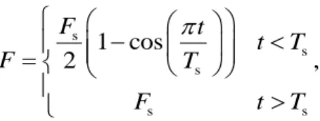
To show that the proposed element was free from locking, the simulation result was compared with an analytical solution. The details of the test are available in [26]. The cantilever beam was quasi-statically bent by a concentrated vertical force applied to its free end. The vertical force was given by
21
s s s s s1 cos
,
2
F
t
t
T
F
T
F
t
T
(26)where Fs = -3100 N and Ts = 4.5 s. In the absence of locking, the deflection of the free end would approach
the static analytical solution given by FsL3/EIyy = -0.0775. The explicit 4th-order Runge-Kutta method was utilized as a time-marching scheme in this simulation and all following simulations. Figure 4 shows the time history of the tip deflection obtained by the proposed beam element. The number of elements was set to 3. As can be observed from the figure, the tip deflection converges to the analytical solution, confirming that the proposed element is free from locking problems.
Fig. 4 Time history of the tip deflection of a quasi-statically bending beam and the analytical static solution FsL3/EIyy = -0.0775.
22
B. Spin-Up Maneuver: Comparison of Different ANCF Beam Elements
To show that the proposed ANCF element produced the same results using smaller generalized coordinates than conventional ANCF elements, a spin-up maneuver of a beam was simulated. The spin-up maneuver is widely used as a bench mark problem [20, 25, 26, 28, 33]. The analysis object was a beam, the parameters of which are available in [20]. One end of the beam was connected to the origin of the global coordinate system through a hinge joint, the axis of which was parallel to the Y-axis. The angle between the beam axis and the X-axis was rotated as follows:
2 2
2
cos
1
<
2
2
>
2
s s s s s s s sT
t
t
t
T
T
T
T
t
t
T
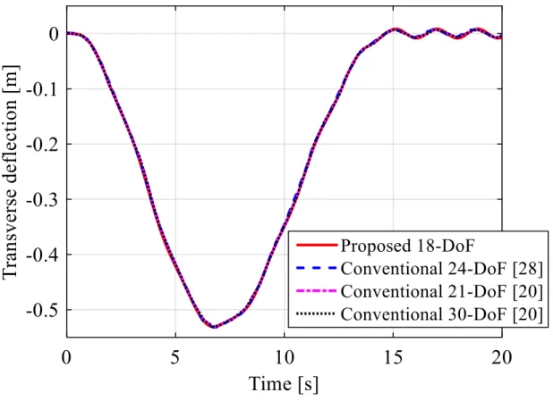
, (27)where Ts = 15 s and ωs = 4 rad/s. The transverse deflection was obtained as the free-end distance between the flexible motion and the prescribed rigid motion. Figure 5 shows the time history of the free-end transverse deflection. The results for the proposed 18-DoF ANCF element were compared with those for the conventional 24-DoF ANCF element [28], 21-DoF, and 30-DoF ANCF elements [20] using locking-free techniques. The results for all four elements were found to be in good agreement. Table 1 gives the numbers of generalized coordinates employed for the spin-up maneuver simulations using the different elements. The proposed element using fewer generalized coordinates produced the same results as the other elements, thereby it cane save computer memory.
23
Fig. 5 Time histories of the transverse deflections in the spin-up maneuver for the different elements.
Table 1 Number of generalized nodal coordinates for the simulation of the spin-up maneuver.
Proposed
18-DoF
element
Conventional
24-DoF
element [28]
Conventional
21-DoF
element [20]
Conventional
30-DoF
element [20]
Number of nodes per element
2
2
3
3
Number of elements
9
8
12
6
Number of generalized
24
C. Rotating Motion: Accuracy Validation of Proposed Element
To further validate the accuracy of the proposed element, its results were compared with those of the GEBF element using Euler angles [34]. The analysis object was a slender beam of length 479 mm, width 50.8 mm, and thickness 0.45 mm. A material density of 4430 kg/m3 and Young’s modulus of 127 GPa were
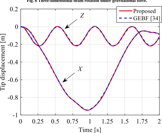
used for the simulation. One end of the beam was connected to the origin of the global coordinate system by a hinge joint, the axis of which was parallel to the Z-axis. The beam axis was initially placed on the X-axis and then rotated with an initial angular velocity π rad/s about the hinge X-axis. At t = 0, the gravitational force began to act in the Z direction. The number of elements was set to 15. Figure 6 illustrates the 3D beam rotation generated by the initial angular velocity and the gravitational force. Figure 7 compares the time histories of the X- and Z-direction tip displacements relative to the initial position for the proposed element and GEBF element. The good agreement confirms the accuracy of the proposed element.
25
Fig. 6 Three-dimensional beam rotation under gravitational force.
Fig. 7 Time histories of the X- and Z- direction tip displacements for the proposed element and GEBF element.
26
D. Aerodynamic Force of Heaving Rigid Wing: Validation of Structural and Aerodynamic Coupling To validate the proposed method for coupling the structural and aerodynamic models, the aerodynamic force determined by the proposed method was compared with that obtained by the VLM solver presented by Parenteau and Laurendeau [29]. The analysis object was a rigid wing with an aspect ratio of 1000. The wing span 2L and chord c were 1000 and 1, respectively. A heaving motion of the rigid wing defined by Z = 0.1 sin(2kV/ct) was simulated using a flow speed V of 1 m/s and reduced frequency k of 0.25. The numbers of chordwise and spanwise aerodynamic panels used for the wing area c × 2L were 10 and 5, respectively. The time step was given by c/(MV ) = 0.1. Figure 8 compares the time histories of the lift coefficient obtained by the proposed method and the VLM solver [29].
Fig. 8 Time histories of the lift coefficient during heaving motion for the proposed method and VLM solver [29].
27
VII
.Experimental Validation
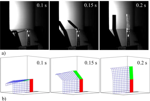
There has been no previous experimental validation of the simulation of wing deployment, especially for very flexible wings. In the present study, we conducted wing deployment experiments in a wind tunnel at IFS, Tohoku University to validate the proposed simulation method. The wind tunnel had an open test section with a regular octagon cross section and a distance of 800 mm between opposite walls.
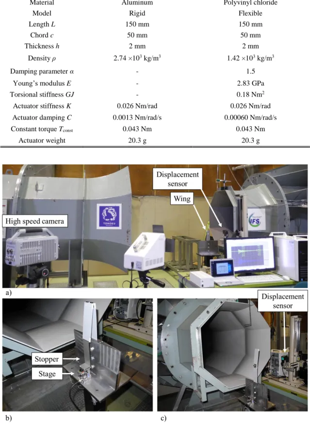
Two experimental models were utilized. One was made from aluminum, and the other from polyvinyl chloride. The second model was used to implement the specific case of a very flexible wing motion coupled with a rigid body motion. Because the aluminum model was much stiffer than the polyvinyl chloride model, the flexible motion (i.e., elastic deformation) of the former was negligibly small. The aluminum model was therefore used to validate the application of the proposed modeling method to a rigid body. The experimental models were composed of two equal bodies connected by a hinge joint with a spring actuator. Table 2 gives the dimensions and material properties of the bodies and spring actuator for the two models. The actuator weight was considered as a lumped mass attached to the outer wing root in the simulation.
Figure 9 shows the folded and deployed experimental models in the wind tunnel. The models were positioned in the vertical direction. The angle of attack was set to zero. The folded state was maintained by a stopper attached to a stage that moved vertically. The stopper did not function when the stage was moved downward. Thus, deployment of the wing was commenced when the stage moved downward. The deployment experiment was conducted for flow speeds of 0–30 m/s in increments of about 5 m/s. The air density was 1.2 kg/m3.
The rigid body motion was measured by a high-speed camera (Photron FASTCAM-X1280PCI) with the sampling period set to 0.0005 s. The elastic bending displacement at the mid-chord point 100 mm from the inner body root was measured by a laser displacement sensor (Keyence LK-G400) with the sampling period set to 0.0002 s.
28
Table 2 Dimensions and material properties of the wing bodies
Property Value
Material Aluminum Polyvinyl chloride
Model Rigid Flexible
Length L 150 mm 150 mm
Chord c 50 mm 50 mm
Thickness h 2 mm 2 mm
Density ρ 2.74 ×10³ kg/m3 1.42 ×10³ kg/m3
Damping parameter α - 1.5
Young’s modulus E - 2.83 GPa
Torsional stiffness GJ - 0.18 Nm2
Actuator stiffness K 0.026 Nm/rad 0.026 Nm/rad Actuator damping C 0.0013 Nm/rad/s 0.00060 Nm/rad/s
Constant torque Tconst 0.043 Nm 0.043 Nm
Actuator weight 20.3 g 20.3 g
Fig. 9 Photographs of the experimental apparatus: a) front view of the measurement systems, and back views of b) folded and c) deployed wings.
29
A. Rigid Wing DeploymentThe simulation and experimental results for the rigid model were compared. Figure 10a shows the deployment motion recorded during the experiment using the high-speed camera for a flow speed of 15 m/s. The camera data was used to determine the deployment time, which is defined as the duration between the commencement of deployment and the time when the two bodies become aligned. The deployment time is an important factor of wing deployment because the aircraft may fall and crash if the wing deployment is not completed within the appropriate time. Figure 11a compares the relationships between the deployment time and the flow speed determined by experiment and simulation. Good agreement can be observed. The deployment time increases with increasing flow speed. This is because the aerodynamic torque acting in the opposite direction of the spring actuator torque increases with increasing flow speed. This can be clearly seen from the decrease in a deployment torque scale
F
T
constT
aero proposed by Fujita and Nagai [7] with increasing flow speed, as shown in Fig. 11b. A smaller deployment torque scale represents a large aerodynamic effect compared to the spring actuator effect. These simulation results were obtained after convergence tests of the aerodynamic model. First, a wake length convergence test was conducted. Consideration of all the wake panels would extend the calculation time, and a wake truncation technique was thus adopted. As expressed by Eq. (19), the effect of the vortex segments far from the collocation point of the wing could be neglected. In other words, the wake beyond a certain distance from the wing could be truncated. This distance is defined as Lw × c. To evaluate the convergence of the wake truncation, we usedthe root mean square (RMS) of the lift coefficient difference, calculated using the time history of the lift coefficient from 0–0.2 s. The lift coefficient error was defined as
all wake L L W all wake L
RMS(
)
Error of
100 [%].
max
C
C
L
C
(28)Here, CL is the lift coefficient obtained from the simulation by truncating the wake at Lw × c, while CLall wake is the lift coefficient obtained from the simulation considering all the wake panels. Figure 12a shows
the relationship between the error and Lw. The error is less than 1% when Lw is greater than 5. Subsequent
simulations were thus conducted using Lw = 5. In the foregoing simulations, the chordwise and spanwise
panels per body were set to 1. A convergence test of the number of chordwise panels M was thus conducted next. The number of spanwise panels N was set to 1 per body. The error of the lift coefficient was defined
30
as =10 L L =10 LRMS(
)
Error of
100 [%].
max
M MC
C
M
C
(29)The value of CL obtained from the simulation with M = 10 was used as the convergence solution. Figure
12b shows the relationship between the error and M, from which it can be seen that the error is less than 1% for M = 2. A convergence test for the number of spanwise panels, N, was also conducted. The number of chordwise panels, M, was set to 1 per body for this convergence test. The lift coefficient error was defined as =10 L L =10 L
RMS(
)
Error of
100 [%].
max
N NC
C
N
C
(30)In this case, the lift coefficient obtained from the simulation with N = 10 was used as the fully converged solution. Figure 12c shows the relationship between the error and N, from which it can be observed that the error is less than 1% for M = 7. Figure 10b shows the results obtained from the simulation using Lw = 5, M
= 2, and N = 7 per body. As can be seen from the figure, the wake is almost flat behind each wing body, and a flat-wake model was thus applicable. Figure 11 shows the simulation results using a flat-wake model, from which good agreement with the results of the free-wake model and experiment can be observed. The calculation time for the flat-wake model was 95% shorter than that for the free-wake model, indicating that the former model is more effective for deployment simulation. The flat-wake model, M = 2, and N = 7 per body was used for the subsequent aerodynamic modeling.
31
Fig. 10 Deployment motions of the rigid model for V = 15 m/s determined by a) experiment and b) simulation.
Fig. 11 Flow speed versus a) deployment time and b) deployment torque scale
F
T
constT
aero.32
Fig. 12 Convergence test results for the a) wake length Lw (M = 1, N = 1), b) number of chordwise
panels, M (N = 1, Lw = 5), and c) number of spanwise panels, N (M = 1, Lw = 5).
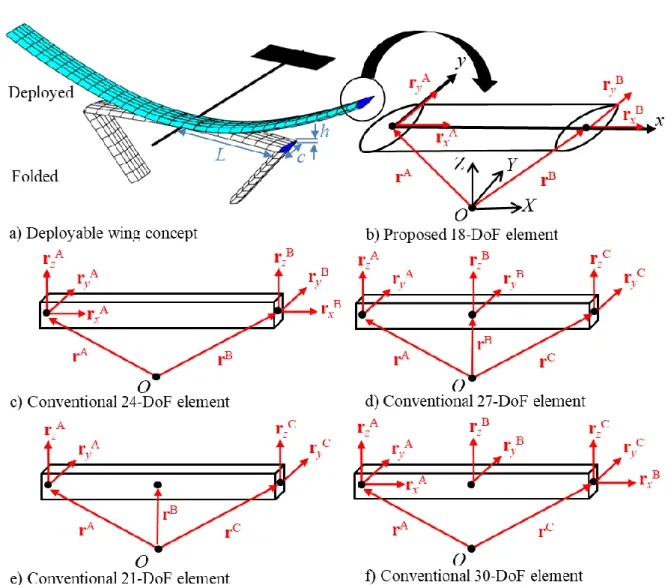
B. Flexible Wing Deployment
The simulation and experimental results for the flexible model were also compared. Figure 13a shows the deployment motion during the experiment measured by the high-speed camera for an flow speed of 10 m/s, while Figure 13b shows the simulation deployment motion. Each wing body in the flexible model was discretized into seven structural elements. Both rigid-body and flexible motions were observed in both the experiment and simulation, with qualitative agreement between the two. To assess the quantitative agreement, we considered the bending deformation at the mid-chord point, which is 100 mm away from the inner body root. Figure 14 shows the time histories of the bending displacements obtained from the experiment and simulation for V = 0, 10, and 20 m/s, which are representative. The minimum displacement (i.e., maximum absolute displacement) was -28 mm, which occurred at 100 mm from the inner wing root after the two bodies became aligned. The experiment and simulation results were found to be in good agreement even when large geometrically nonlinear deformations occurred. Figure 15 shows the
33
relationship between the flow speed and the maximum displacement during the deployment defined as D, as shown in Fig. 14. Here, D is used as a representative value to show the displacement during the deployment. The maximum displacement D during the deployment decreases with increasing flow speed. This is because the aerodynamic damping force increases with increasing flow speed. As can be observed from Fig. 15, the simulation and experiment are in good agreement.
Fig. 13 Deployment motions of the flexible model for V = 10 m/s obtained from the a) experiment and b) simulation.
34
Fig. 14 Time histories of the bending displacement at the mid-chord 100 mm from the inner wing root for a) V = 0 m/s, b) V = 10 m/s, and c) V = 20 m/s.
35
VIII. Conclusion
A multifidelity multibody modeling method based on a new ANCF beam element for slender deployable wings was developed in the present study. First, two drawbacks of the conventional ANCF beam element, namely, the use of a large number of generalized coordinates and the problem of numerical locking, were resolved through the utilization of asymmetrically gradient-deficient nodal coordinates and internal constraint equations. The quasi-static bending simulation of the proposed element converged to the analytical solution, which demonstrated that the proposed element is free from locking. The proposed element using fewer generalized coordinates could provide the same result as the conventional elements. This showed that the proposed element had a better computational efficiency. By comparison of the proposed element with the GEBF element, the proposed ANCF element was confirmed to be accurate.
The proposed modeling method also facilitates computationally efficient rigid multibody simulation and more realistic flexible multibody simulation using a consistent modeling procedure and the same simulation program architecture. This further enables the use of the same structural-aerodynamic coupling method for both rigid and flexible multibody models. We demonstrated the coupling using the UVLM aerodynamic model and the easy development of the UVLM aerodynamic panels from both the rigid and flexible models using a shape function. Wing deployment experiments were also performed in a wind tunnel to validate the results of the coupling simulation. Both rigid and very flexible physical wing models were considered in the experiments. The results of the rigid/flexible multibody simulations were found to be in good agreement with those of the wind tunnel experiments. We also demonstrated that the flat-wake model was effective for the deployment simulation. The simulation with the flat-wake model was in good agreement with the experiment and had a 95% shorter calculation time than that with the free-wake model. This study represents the first acquisition of experimental data on very flexible wing deployment involving large geometrically nonlinear deformations. This experimental data would be useful for validating various dynamic simulations of very flexible multibody systems under aerodynamic forces.
36
Funding
Japan Society for the Promotion of Science (JSPS) (18K18905)
Collaborative Research Project of the Institute of Fluid Science, Tohoku University.
Acknowledgments
This work was supported by the Japan Society for the Promotion of Science (JSPS) KAKENHI (Grant Number 18K18905). The wing deployment experiments were performed under the Collaborative Research Project of the Institute of Fluid Science (IFS), Tohoku University. We acknowledge the use of the IFS wind tunnel facility for the experiments.
References
[1] Attar, P. J., Tang, D., and Dowell, E. H., “Nonlinear Aeroelastic Study for Folding Wing Structures,”
AIAA Journal, Vol. 48, No. 10, 2010, pp. 2187–2195.
doi:10.2514/1.44868
[2] Braun, R. D., Wright, H. S., Croom, M. A., Levine, J. S., and Spencer, D. A., “Design of the ARES Mars Airplane and Mission Architecture,” Journal of Spacecraft and Rockets, Vol. 43, No. 5, 2006, pp. 1026–1034.
doi:10.2514/1.17956
[3] Fujita, K., and Nagai, H., “Comparing Aerial-Deployment-Mechanism Designs for Mars Airplane,”
Transactions of the Japan Society for Aeronautical and Space Sciences, Vol. 59, No. 6, 2016, pp.
323–331.
doi:10.2322/tjsass.59.323
[4] Thai, Z., Coles, S., Jacob, J. D., Duncan, B., Dancer, C., Hudson, A., Thomas, L., and Allen, M., “Never-EVER Land - A Titan Flyer Concept,” 2018 AIAA Aerospace Sciences Meeting, AIAA Paper 2018-1535, 2018.

![Fig. 8 Time histories of the lift coefficient during heaving motion for the proposed method and VLM solver [29]](https://thumb-ap.123doks.com/thumbv2/123deta/5921180.1051228/27.892.149.719.527.970/time-histories-coefficient-heaving-motion-proposed-method-solver.webp)