九州大学応用力学研究所 Reports　No.150（Mar. 2016）

全文

(1)ISSN 1345-5664. 九州大学応用力学研究所所報. No. 150 March 2016.

(2) CONTENTS. Numerical analysis of dislocation density and residual strain in multicrystalline silicon for solar cells using experimental verification By Satoshi NAKANO, Bing GAO, Karolin JIPTNER, Hirofumi HARADA, Yoshiji MIYAMURA,. Takashi. SEKIGUCHI,. Masayuki. FUKUZAWA. and. Koichi. KAKIMOTO……………………………………………………………………………….......... 1. Compilation of bathymetric data of the East China Sea By Katsuto UEHARA............................................................................................................ 6 Significant impacts of heterogeneous reactions on the chemico-physical properties of dust particles during severe dust events over East Asia in 2015 By Zhe WANG, Xiaole PAN, Jie LI, Zifa WANG, Pingqing FU, Ting YANG, Hiroshi KOBAYASHI, Atsushi SHIMIZU, Nobuo SUGIMOTO, Shigekazu YAMAMOTO and Itsushi UNO……………………………………………………………………….........……...14 High-Resolution LES of Undulating Motions behind the Wind Turbine Using the Actuator Line Technique By Takanori UCHIDA..........................................................................................................25 Analysis of the Airflow Field over Real Terrain with Commercially-Available CFD Software By Takanori. UCHIDA,. Tatuso. AOYAGI,. Fumihito. WATANABE. and. Shin. MIKAMI..........................................................................................................................34 Wind Conditions Investigation about a Small Wind Turbine Accident By Takanori UCHIDA....…………………………………………………………………….........40 Reproducibility of Complex Turbulent Flow Using Commercially-Available CFD Software ―Report 1: For the Case of a Three-Dimensional Isolated-Hill With Steep Slopes― By Takanori UCHIDA..........................................................................................................47 Reproducibility of Complex Turbulent Flow Using Commercially-Available CFD Software ―Report 2: For the Case of a Two-Dimensional Ridge With Steep Slopes― By Takanori UCHIDA..........................................................................................................60.

(3) Reproducibility of Complex Turbulent Flow Using Commercially-Available CFD Software ―Report 3: For the Case of a Three-dimensional Cube― By Takanori UCHIDA……………………………………………………………………………..71.

(4) Reports of Research Institute for Applied Mechanics, Kyushu University No.150 (1 – 5) March 2016. Numerical analysis of dislocation density and residual strain strain in multicrystalline silicon for solar cells using experimental verification Satoshi NAKANO*1, Bing GAO*1, Karolin JIPTNER*2, Hirofumi HARADA*2, Yoshiji MIYAMURA*2, Takashi SEKIGUCHI*2, Masayuki FUKUZAWA*3 and Koichi KAKIMOTO*1 E-mail of corresponding author: [email protected] (Received January 7, 2016). Abstract A three-dimensional (3D) Haasen-Alexander-Sumino model (HAS model) has been developed to study the dislocation density and residual strain in the crystal. We compared the difference between calculation results and experimental results. The results show that the HAS model can evaluate the dislocation density and residual strain in the crystal semiquantitatively. And the residual strain for a multicrystal is lower than that for a mono-like crystal, while the dislocation density for the multicrystal is higher than that for the mono-like crystal. In the case of mono-like crystal, the dislocation generation is small and the thermal stress cannot relax easily, then residual strain is high. In the case of the multicrystal, the dislocation generation is large and there are so many grains, then the thermal stress can relax easily and residual strain is low. Keywords Keywords : Silicon, Solar cell, Directional solidification, Dislocation, Strain. 1. Introduction In recent years, photovoltaic energy is essential to solve the energy issues and environmental problems which we confront. For widespread utilization of the photovoltaic application in the world, it is important to fulfill the demand of cost reduction and improvement of conversion efficiency. The directional solidification method is important and most prevailing method for growing multicrystalline silicon (mc-Si) ingots for photovoltaic materials. Major advantages of this method are low cost and high throughput for photovoltaic production. However, seeded directional solidification method (seed-cast) 1-3) has been a focus of constant attention. Mono-like Si ingots are grown from seed crystals, which are putted at the bottom of the crucible using the directional solidification method. These days, the conversion efficiency of mono-like Si is about the same that of monocrystalline Si, which is grown by the. *1 Research Institute for Applied Mechanics, Kyushu Univ. *2 National Institute for Materials Science *3 Kyoto Institute of Technology. Czochralski (CZ) method4) . For mc-Si or mono-like Si, which is grown by the directional solidification method, it is widely known that high dislocation density is main problem to decrease conversion efficiency5, 6), while residual stress can cause the crystals to fracture 7, 8). For increasing both conversion efficiency and yield rate of solar cells, the dislocation density and residual stress in the crystal needs to be improved. For experimental method, it is important to evaluate the quality of crystals 9-12), but this cannot be estimated how to generate dislocation and residual stress during the growth process. Numerical simulation is a powerful tool to provide us a valuable perception by analyzing calculation results of the crystal during the growth process. Therefore, we can improve the furnace design and optimize the growth condition, which are effective to the quality of the crystal, by numerical simulation. A 3D Haasen-Alexander-Sumino model (HAS model) has been developed 13-17) to study the behavior of dislocation and residual strain during the growth process. We assumed the silicon crystal was isotropic, crystal anisotropy was neglected. In this study, we pay attention to the HAS model can be used to calculate dislocation density and residual strain for mono-like Si and mc-Si even we assumed the silicon crystal was isotropic. And.

(5) 2. Nakano et al.: Numerical analysis of dislocation density and residual strain in multicrystalline silicon for solar cells using experimental verification. we analyzed the relationship between the dislocation density and residual strain using this model.. 2.. v0 = 5000m / s , τ 0 = 1MPa , m = 1 , 23) , U = 2.2eV kb = 8.617 ×10−5 eVK −1 . The effective stress is given by: where. Computation Method. τ eff(α ) = τ (α ) − τ i(α ) − τ b(α ). The directional solidification furnace consisted of a silicon melt, a crystal, crucibles, pedestals, heat shields, and heaters. The crystal had a height of 75 mm and a diameter of 105 mm. A transient global model was developed for the directional solidification process to investigate the global heat transfer in the entire furnace as a function of time. Global heat transfer in the entire furnace included the convective heat transfer of the silicon melt, the conductive heat transfer in all of the solid components, and the radiative heat transfer in all of the diffusive surfaces of the furnace. A dynamic interface tracking method was also included to obtain the shape of the solid–liquid interface. Details of the calculations have already been reported elsewhere18-20). A 3D HAS model was also investigated using the temperature distributions in the crystal which we calculated. A brief explanation of the formulas as follows. Details of the calculations can be found elsewhere13-17). A silicon crystal has twelve slip directions because of its fcc structure17, 21) . The resolved shear stress τ(α) in the α slip direction can be obtained using the tensor transformation technique21) . The creep strain rate is obtained by Orowan’s relationship as follows 22):. dε. (α ) pl. dt. = N m(α ) v (α )b. (1). where Nm is the mobile dislocation density, b is Burger’s vector, and v is the slip velocity of the dislocation. The rate of the mobile dislocation density in the α slip direction is given as follows:. dN m(α ) (α ) = KN m(α ) v (α )τ eff dt (α ) + K * N m(α ) v (α )τ eff ∑ fαβ N m( β ) − 2rc N m(α ) N m(α )v(α ). (2). where τeff is the effective stress for dislocation multiplication, K and K* are multiplication 15-17) constants , and rc is the effective dipole half width15-17). The fαβ coefficients are given either as one or zero. The slip velocity of the dislocation v is given by:. τ eff(α ) m U ) exp( − ) τ0 kbT. v (α ) = v0 (. where τ (α ) is the resolved shear stress, τ i(α ) is the stress for overcoming short-range obstacles, and τ b(α ) is the internal long-range elastic stress which is caused by mobile dislocations15-17, 23). The short-range and long-range interactions are given as follows23) :. τ i(α ) = µb. (3). ∑β aαβ ( N β. ( ) m. + Ni( β ) ). τ b(α ) = µb∑ Aαβ Nm( β ). (5). (6). β. where aαβ and are Aαβ the interaction coefficients23). Because the dislocation densities and creep strains for all of the slip directions are obtained, the total dislocation density and total creep strain can be expressed as: 12. N m = ∑ N m (α ). (7). α =1. 12. ε pl = ∑ ε (plα ) α =1. 1 (α ) (n ⊗ m(α ) 2. (8). +m(α ) ⊗ n (α ) ) sign(τ (α ) ) where n (α ) is the normal unit vector of the slip plane and m (α ) is the unit vector of the slip direction. The following assumptions were made: (1) the boundary condition at the solid–liquid interface was a no traction boundary, and (2) the boundary conditions at the crystal-crucible wall interfaces were also no traction boundaries because a coating was used between the silicon melt and the quartz crucible in order to reduce the effect of the crucible.. 3.. β ≠α. (4). Results and discussion. We used one of major crystal growth methods based on the directional solidification process; the traveling heater method. In the traveling heater method, the heaters were moved upward in order to grow the crystal, while the heater power was held constant until completion of the solidification process, at which point it was decreased..

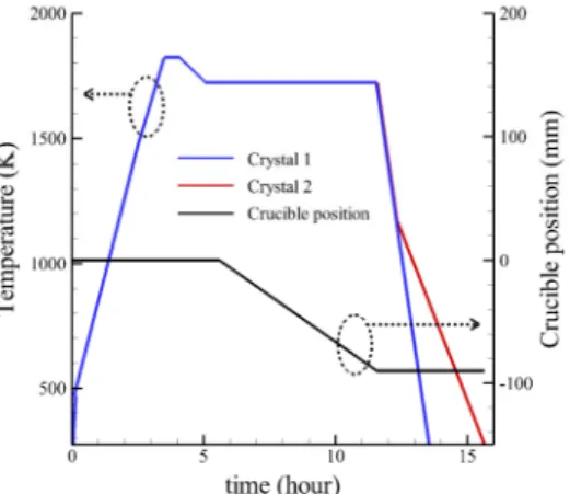
(6) Reports of Research Institute for Applied Mechanics, Kyushu University No.150 March 2016 Two mono-like crystals (Crystal 1 and Crystal 2) were grown by the traveling heater method using (001)-oriented seed crystals10, 11) . Figure 1 shows the growth recipe of heater temperature and crucible position for the experiment 11) . We conformed to the melting and solidification process for two crystals and only changed the cooling rate during the cooling process below 900 °C. The cooling rate for Crystal 1 was about 12 °C/min, whereas that for Crystal 2 was about 5 °C/min below 900 °C. Figures 2 (a) and 2(b) are the optical images of Crystal 1 and Crystal 2. Two ingots were cut 1.5 mm thickness at vertical direction with (110) surface to measure the dislocation density and residual strain in the ingot. Crystal 1 has a large area of mono crystal which grew from the seed crystal; however Crystal 2 has a large area of multicrystal which originated from the side wall. The measurement of residual strain was performed using a scanning infrared polariscope (SIRP). Details of the SIRP measurement can be found in publications24, 25). We also calculate temperature distribution in the crystal with following parameters. The cooling rate for Crystal 1 was about 6.1 °C/min, whereas that for Crystal 2 was about 2.2 °C/min below 900 °C. The cooling rate between experiment and calculation is different; however, we can verify the effect of the cooling rate below 900 °C qualitatively.. 3. Figure 3 shows the distribution of dislocation density in the periphery of the crystals with respect to the ingot height in the calculation results and experimental results. The previous 2D calculation results are different from the experimental results by one order of magnitude. However, our new 3D calculation results are very close to the experimental results. The calculation results for Crystal 1 and Crystal 2 are almost the same because the dislocations were mainly generated at the high-temperature region in the HAS model and because our calculations did not take into account for the dislocation propagation and movement. Therefore, the distribution of dislocation density for Crystal 1 and Crystal 2 is almost the same because the cooling rate changed at 900 °C, which is not a high-temperature region.. Fig. 3 The distribution of dislocation density in the periphery of the crystal with respect to the ingot height in the calculations and the experiments.. Fig. 1 The growth recipe of heater temperature and crucible position for the experiment.. (a). (b). Fig. 2 Optical images of (a) Crystal 1 and (b) Crystal 2.. Figures 4(a) and 4(b) show SIRP images of Crystal 1 and Crystal 210, 11). Figures 5(a) and 5(b) show the distribution of residual strain of Crystal 1 and Crystal 2 for calculation results. From Fig. 4(a) and Fig. 5(a), both residual strain distributions are symmetric distribution and quite similar. And the higher strain in the crystal is periphery and lower strain is in the center. These results suggest that the peripheries in the crystal are the areas of high temperature gradients and therefore the high thermal stresses are in those areas. From Fig. 2(b), 4(b) and 5(b), even multicrystal area in the ingot is large, the distribution of residual strain for calculation result is close to that for experimental result. Figures 6(a) and 6(b) show an optical image and SIRP image of multicrystalline silicon ingot10). The solidification and cooling process is the same as Crystal 1. Even there are so many grains, the distribution of residual strain as shown in Fig. 5(a) is close to the SIRP image as shown in Fig. 6(b). Figures 7(a) and 7(b) show the distribution of residual strain in the center and.

(7) 4. Nakano et al.: Numerical analysis of dislocation density and residual strain in multicrystalline silicon for solar cells using experimental verification. (a). (b). Fig. 4 SIRP images of (a) Crystal 1 and (b) Crystal 2.. (a). (a). (b). Fig. 5 The distribution of residual strain in (a) Crystal 1 and (b) Crystal 2 in the calculations.. (a). (b). Fig. 6 (a) Optical image and (b) SIRP image of the multicrystalline silicon ingot. periphery of the crystal with respect to the ingot height for the calculation and experimental results. The distribution of residual strain for Crystal 1 and Crystal 2 in calculation result is close to that for experimental result. And the difference of residual strain between Crystal 1 and Crystal 2 is small. The distribution of residual strain for multicrystal ingot is also close to that for calculation results. And residual strain for multicrystal ingot is lower than that for mono-like ingot Crystal 1 and Crystal 2. The average dislocation density in whole of the crystal for Crystal 1, Crystal 2 and multicrystal is 0.5x10 5, 1.1x105, and 1.5x10 5 cm-2 respectively26). The average dislocation density for multicrystal is higher than that for mono-like Crystal 1 and 2. This phenomenon is owing to the relationship between the dislocation density and the residual strain in the crystal. For the mono-like crystal, because dislocation generation is small, thermal stress cannot easily relax and the residual strain is high. In contrast, for the multicrystal, because dislocation generation is large and there are many grains, the thermal stress can easily relax, and therefore the residual strain is low. In case of increasing the size of crystal, difference of. (b) Fig. 7 The distribution of residual strain in the (a) center and (b) periphery of crystal with respect to the ingot height in the calculations and experiments. residual strain between mono-like crystal and multicrystal could be increased. Therefore, we can expect the difference of residual strain could be more effective to dislocation density. Thus, even multicrystal area in the ingot is large, HAS model is very useful to expect the distribution of dislocation density and residual strain semiquantitatively.. 4.. Conclusion Conclusion. A 3D Haasen-Alexander-Sumino model has been developed and compared with experimental results performed in mono-like and multicrystal silicon ingots to study the relationship between dislocation density and residual strain in the crystal. The calculation results are good agreement with the experimental results even crystal has large multicrystal area. From these results, the HAS model is very useful model to evaluate dislocation density and residual strain in the crystal semiquantitatively. And we verified the relationship between dislocation density and residual strain in the crystal using numerical analysis in comparison with.

(8) Reports of Research Institute for Applied Mechanics, Kyushu University No.150 March 2016 experimental results.. Acknowledgement This work was partly supported by the New Energy and Industrial Technology Development Organization (NEDO) under the Ministry of Economy, Trade and Industry (METI).. 10). 11). 12). References 1). 2). 3). 4). 5). 6) 7) 8) 9). N. Stoddard, B.Wu, I.Witting, M.Wagener, Y.Park, G.Rozgonyi, R.Clark, Solid State Phenom. 131 (2008) 1. Y. Miyamura, H. Harada, K. Jiptner, J. Chen, R.R. Prakash, J.Y. Li, T. Sekiguchi, T. Kojima, Y. Ohshita, A. Ogura, M. Fukuzawa, S. Nakano, B. Gao, K. Kakimoto, Solid State Phenom., 89 (2013) 205. B. Gao, S. Nakano, H. Harada, Y. Miyamura, T. Sekiguchi, K. Kakimoto, Journal of Crystal Growth, 352(1), (2012) 47. Takahiro Arima, Takemichi Honma, Shin Sugawara and Yasuhiro Matsubara, 6th World Conference on Photovoltaic Energy Conversion, Kyoto, Japan, p511, 2014. K. Arafune, T. Sasaki, F. Wakabayashi, Y. Terada, Y. Ohshita, M. Yamaguchi, Physica., B 376-377 (2006) 236. M. M’Hamdi, E. A. Meese, E. J. Ovrelid, and H. Laux, Proceedings 20th EUPVSEC (2005) 1236. S. Nakano, B. Gao, K. Kakimoto, J. Cryst. Growth, 318 (2011) 280. M. M’Hamdi, S. Gouttebroze, and H. G. Fjar, J. Cryst. Growth, 318 (2011) 269. Y. Miyamura, J. Chen, R. Prakash, K. Jiptner, H.. 13) 14) 15) 16) 17) 18) 19) 20) 21) 22) 23). 24) 25) 26). 5. Harada, T. Sekiguchi, Acta Phys. Pol. A 125[4] (2014) 1024. K. Jiptner, M. Fukuzawa, Y. Miyamura, H. Harada, and T. Sekiguchi, J. J. Applied Physics, 52(2013) 065501. K. Jiptner, M. Fukuzawa, Y. Miyamura, H. Harada, K. Kakimoto, and T. Sekiguchi, Physica Status Solidi C, 10 (2013) 141. M. Trempa, C.Reimann, J.Friedrich, G.Muller, D.Oriwol, J.Cryst.Growth 351 (2012) 131. H. Alexander, P. Haasen, Solid State Physics, 22 (1968) 27. M. Suezawa, K. Sumino, I. Yonenaga, J. Appl. Phys., 51 (1979) 217. B. Gao, S. Nakano, H. Harada, Y. Miyamura, K. Kakimoto, Cryst. Growth Des., 13 (2013) 2661. B. Gao and K. Kakimoto, J. Cryst. Growth, 384 (2013) 13. B. Gao and K. Kakimoto, J. Cryst. Growth, 396 (2014) 7. L. J. Liu, S. Nakano, and K. Kakimoto, J. Cryst. Growth, 282 (2005) 49. K. Kakimoto, L. J. Liu, and S. Nakano, Mater. Sci. Eng., B134 (2006) 269. L. J. Liu, S. Nakano, and K. Kakimoto, J. Cryst. Growth, 292 (2006) 515. N. Miyazaki, Y. Kuroda, M. Sakaguchi, J. Cryst. Growth, 218 (2000) 221. E. Orowan, Philos. T. Roy. Soc., A 52 (1940) 8. J. Cochard, I. Yonenaga, S. Gouttebroze, M. M’Hamdi, Z. L. Zhang, J. Appl. Phys. 107 (2010) 033512. M. Fukuzawa, M. Yamada, R. Islam, J. Chen, and T. Sekiguchi: J. Electron. Mater. 39 (2010) 700. M. Yamada: Rev. Sci. Instrum. 64 (1993) 1815. K. Jiptner, private communications..

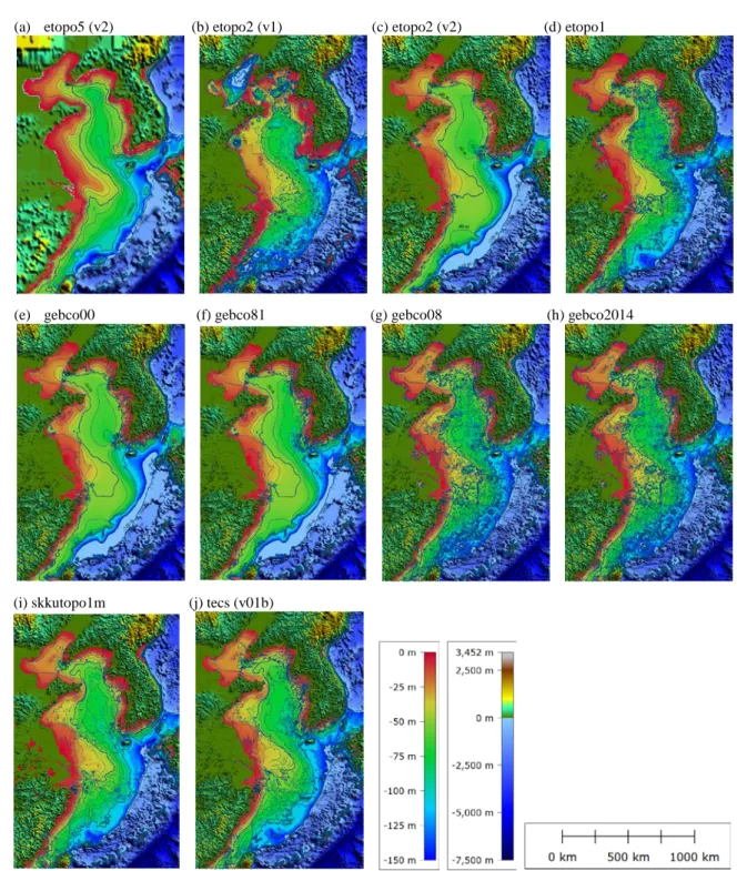
(9) Reports of Research Institute for Applied Mechanics, Kyushu University No.150 (6 –13) March 2016. Compilation of bathymetric data of the East China Sea Katsuto UEHARA*1 E-mail of corresponding author: [email protected] (Received January 29, 2016). Abstract One arc-minute resolution grid bathymetry of the East China Sea has been developed by compiling a large number of sounding data derived from various sources. The dataset was found to retain advantages of two existing grid bathymetries: representing basic bottom features found in navigational charts as in skkutopo1m dataset, while it resolves detailed bottom features observed in gebco2014 gridded bathymetry. Through comparisons between new and nine existing datasets, spurious bottom features in previous datasets were identified in near-coast regions and in areas where the source data were sparsely distributed. The verification also has clarified the regions where additional sounding records are required to improve the data quality. Keywords : Bathymetry, East China Sea, Digital Terrain Model, continental shelf. 1.. Introduction. Even though bathymetry is one of the most important properties which regulate the dynamics of coastal seas, uncertainty still exists in our knowledge on the depth of shallow marginal seas. It is partly because typical spatial scales of bottom features in shallow seas are so small that the features may often slip through the networks of satellite and in-situ survey lines. The amount and quality of available sounding data have been much less than those required to map the whole sea area. The situation, however, has greatly improved in the last decade. Many countries in East and Southeast Asia have initiated intensive sounding surveys for mapping purpose, and increasing number of detailed navigational charts have newly published especially in the last several years. Furthermore, recent scientific surveys using multi-beam soundings also have provided detailed bathymetric information. This study compiles a gridded bathymetry of the East China Sea (ECS) including the Bohai and Yellow seas by utilizing a large number of sounding data, many of which have been published recently. The aim of this study is to produce a bathymetric map of the ECS which can resolve features having a spatial scale of 5-10 km, and to evaluate the reliability of bathymetric data of the ECS. Similar grid bathymetry of the South China Sea is presented in another article1).. 2.. Materials and methods. *1 Research Institute for Applied Mechanics, Kyushu Univ.. 2.1 Existing bathymetric datasets Table 1 is a list of gridded bathymetric datasets covering the East China Sea (ECS) which provide depths at data points defined on a longitude-latitude grid. The existing datasets fall into three streams. Etopo series are global grid data distributed by U.S. National Centers for Environmental Information (NCEI). The first etopo product published in 1988, etopo52), has a spatial resolution of 5 minutes (1/12 degrees) and was superseded by etopo23) (2 min resolution) in 2001 and further by etopo14) (1 min resolution) in 2009. While etopo5 referred to in-situ sounding records, etopo2 and etopo1 rely mostly on satellite altimetry techniques5) which have greatly improved the quality of water depths in deep oceans. In this study, the revised edition of etopo5 issued in 19906), the first3) and second7). Table 1 List of bathymetric datasets covering ECS Name etopo5 etopo2 etopo1 gebco00 gebco81 gebco08 gebco2014 skkutopo1m tecs. Res 5min 2min 1min 1min 1min 0.5min 0.5min 1min 1min. Released 19882) (19906)) 20013) (20067)) 20094) 20038) 20089) 200910) 201411) 200212) 2016. Coverage global global global global global global global East Asia ECS.

(10) Reports of Research Institute for Applied Mechanics, Kyushu University No.150 March 2016 (issued in 2006) edition of etopo2 and the grid-registered version of etopo14) were examined. Gebco (General Bathymetric Chart of the Oceans) gridded bathymetries have been distributed by British Oceanographic Data Centre (BODC). In this study, we verified gebco centenary edition issued in 20038) (1 min res; referred to as gebco00 hereafter), gebco one minute grid last updated in Nov. 20089) (1 min res; gebco81), gebco_08 version 2010092710) (0.5 min res, first release appeared in Jan. 2009; gebco08) and gebco_2014 version 2015032511) (0.5 min res, initial version published in Nov. 2014; gebco2014). A dataset that belongs to the third stream is SKKUtopo1m12) (1 min res, published in 2002) compiled from in-situ sounding data. Unlike etopo and gebco global datasets, its geographical coverage is limited to East Asia (117°E143°E and 24°N-52°N). We did not use two Japanese gridded datasets, i.e., JEGG50013) issued by Japan Oceanographic Data Center (JODC) covering the southern and southwestern ECS (122°E132°E and 24°N-30°N; 128°E-144°E and 30°N-38°N) in a resolution of 500 m and JTOPO30v214) published by Marine Information Research Center (MIRC), Japan Hydrographic Association (JHA) which covers 120°E-150°E and 18°N-48°N in 0.5-minute interval. It was because the former was supplied in spatiallysmoothed form and did not conform with some raw sounding data, while the latter was focused mainly on deep oceans adjacent to Japanese waters so that only a limited number of sounding records were used to map the main shallow portion of the ECS.. 2.2 Tecs bathymetry The regional bathymetry compiled in this study, tecs, provides heights over an area ranging 116°E-131°E and 24°N-42°N in a resolution of 1 minute. Tecs covers the whole ECS and the westernmost part of the Japan Sea. For an area west of 125°E and south of 27°N, the dataset is compatible with the South China Sea bathymetry, tscs1). The dataset focuses mainly on the continental shelf shallower than 200m, which comprises more than 70% of the ECS area and an effort was made to resolve bottom features having a spatial scale of 5-10 km, a typical width of submarine linear sand ridges found at various locations in the ECS. Compilation of the dataset was made under two concepts. In contrast to other global datasets keeping a universal quality standard over a wide area by applying a spatial filter, tecs was compiled on a best-effort basis, i.e., pursuing the best quality at each locality by utilizing as many source data as possible. Furthermore, a care was taken to avoid generating spurious depth values, which was accomplished by adopting a. 7. conservative interpolation scheme and by excluding extreme sounding values, e.g., depth at the top of a small and isolated seamounts which does not represent the water depth of the region.. 2.3 Data source In this study, only in-situ sounding data were used to compile the sea portion of tecs. The primary source of the sounding data was electronic and paper charts issued by local countries (China, South Korea, Japan and Russia), electronic charts by U.K. and paper charts by U.S. As for Chinese and Korean waters, we used substantially all the electronic charts categorized as Harbour, Approach and Coastal scales (1:10k to 1:300k) available at Dec. 2015 and adopted the version issued at around Feb. 2012 when available to retain the consistency among the charts. Paper charts were scanned and converted into WGS84 coordinates if necessary. In addition, a large number of single-beam sounding records in Japanese waters collected by Japan Coast Guard, as well as multi-beam sounding data at regions east of Taiwan and in the Japan Sea south of 38°N were used to generate the dataset. The multi-beam data were converted into grid-point data having a spacing of 0.2 minutes because the original resolution was too high for the current purpose. For the land portion, we used GLOBE dataset15), a global gridded topography dataset provided in 0.5minute interval. Fig.1 illustrates the number of source data that fall into 5 minute bins. Aside from nearshore regions, the sounding data were densely distributed in areas west and southwest of Korean Peninsula, west of Taiwan and in the southern part of the Japan Sea. It is to be noted that many of the data found in these area have been originated from electronic charts and multi-beam products published in the last five years.. 2.4 Data processing All the paper and electronic charts were displayed on a computer screen and the depth points were digitized into xyz (longitude, latitude and depth) format. The obtained data were compared with other sounding records supplied in digital form. It is to be noted that not all the depths indicated in the charts were adopted for the data compilation. Incorporating all the depths indicated in electronic charts, which was conducted in a pilot study, resulted in a generation of a grid bathymetry having depths shallower than those observed. It was because navigational charts tend to indicate the shallowest.

(11) 8. Uehara: East China Sea bathymetric data. (a). (b). Fig. 1 Histogram showing the number of sounding data used for compilation included in 5 min bins. Bins without any sounding data are indicated in white colors. Note the number of data in a bin is not limited to 25 and may exceed 1000.. Fig. 2 Bathymetric relief off the west coast of Kyushu Island created (a) with and (b) without using singlebeam sounding depths along survey lines indicated in red dots. Depth values and a navigational chart (Japanese chart W180) are overlain for reference.. depth in a specific area than depths representing a certain region. A care was taken to adopt depth values representing the area especially at places where sounding data were sparsely distributed. Depth contours were not digitized unless contours (1) mark the location of a steep slope where the depth changes greatly or (2) represent the extent of elongated shoals or trenches where depths vary in anisotropic manner, because the contours generally differ among charts. Single-beam sounding records were verified by comparing with other depth data. Some of the records obtained from several particular cruises were not adopted in this study because they show depths systematically different from those observed at surrounding locations and inclusion of such dataset may often produce artificial features (Fig. 2). Some of the multi-beam records also indicate erroneous values especially at shallow regions and along the edge of a swath band. It was therefore necessary to verify the data carefully before being used as a part of the source data. The gridded land data were introduced to fill hollow areas devoid of input data, which helped generating realistic bathymetries around land features such as promontories and islands where. coastlines were intricate or were closed. All the sounding records and the topographic grids were combined together and converted into a grid data having a spacing of 1 minutes which was made by applying Natural Neighbor interpolation scheme of Surfer 13 application (Golden Software). This scheme does not generate values beyond the range of the actual dataset. In this study, we have chosen this conservative interpolation method to avoid generating spurious features, with the cost of losing some information contained in the original sounding data.. 3.. Results. Fig. 3 shows the bathymetry of the ECS derived from the existing and newly developed datasets. Here we focus on shallow regions and depths between 0 m and 150 m are drawn with a separate color scale. It was found that all datasets show depth pattern slightly different among each other in the shallow portion of the ECS. An exception is the bathymetry of gebco08 and gebco2014 (Figs. 3g and 3h) which differ only in a deep area south of Ryukyu Islands. Another exception is etopo2 (v1) bathymetry (Fig. 3b): depths in some regions deviates largely from those found in other datasets, e.g., depth exceeding 200 m in the central Bohai Sea, the northern Yellow Sea and Haizhou Bay,.

(12) Reports of Research Institute for Applied Mechanics, Kyushu University No.150 March 2016 (a) etopo5 (v2). (e) gebco00. (i) skkutopo1m. (b) etopo2 (v1). (f) gebco81. (c) etopo2 (v2). (d) etopo1. (g) gebco08. (h) gebco2014. 9. (j) tecs (v01b). Fig. 3 Depth distribution around the ECS derived from ten different bathymetric datasets (the list of the datasets is found in Table 1). Depth contours were drawn for every 10 m from 10 to 100 m, 120 m, 150 m and 200 m depth. The color scale in the left hand side applies to depth range 0-150 m, whereas the scale in the right is used in other heights/depths.. while depths being too shallow along the western and southern coasts of Korea. These apparent errors found in etopo2 (v1) were modified in the second version (Fig. 3c). Etopo5 (v2) bathymetry (Fig. 3a) based on in-situ sounding data showed depth pattern somewhat similar to those found in navigational charts, except in area off Jiangsu coasts where an extensive inner shelf was not existent and in the. Yangtze Shoal where the depth seems to be shallower than observed. These discrepancies may have caused because detailed depth information around two areas were not available at the time the dataset was published. In etopo2 (v2) and etopo1 (Figs. 3c and 3d), the extent of nearshore region shallower than 20 m and the representation of water depths in the Yangtze Shoal seems to have improved.

(13) 10. Uehara: East China Sea bathymetric data. (a) etopo1. (b) gebco2014. (c) skkutopo1m. (d) tecs (v01b). Fig. 4 Depth distribution off southwest Korea for (a) etopo1, (b) gebco2014, (c) skkutopo1m and (d) tecs bathymetries. Contour lines are drawn for every 20 m and lines indicated in a light green color denote depths greater than 100 m. Note that a color scale is different from the one used in Fig. 3. when compared to etopo5 (Fig. 3a). On the other hand, these new datasets do not seem to represent areas deeper than 40 m properly. In addition, a spurious shoal has emerged in an area south of Jiaozhou Bay in etopo2 (v2) and etopo1. Though etopo1 implies many small-scale structures compare to etopo2, it was not clear whether these features are realistic ones. An apparent jump of 50 m contour across latitude 30°N off Hangzhou Bay found in etopo1 is probably related to the northern limit of a Japanese gridded bathymetry used in etopo1 which did not have enough accuracy outside Japanese waters. While the depth patterns of gebco00 (Fig. 3e) were virtually the same with that of etopo2 (v2) (Fig. 3c), those in the Korean side of the Yellow Sea were modified in its revised. edition, gebco81 (Fig. 3f). The contour pattern of gebco81 in the modified area resembles more to that of etopo5 than to etopo2 (v2). Gebco08 and gebco2014 bathymetries (Figs. 3g and 3h) generally show more realistic contour patterns, in terms of the similarity with those presented in navigational charts, compared to etopo and previous gebco bathymetries. A significant improvement was observed for the bathymetry in the Bohai Sea and the overall shape of the Yangtze Shoal. These 1/2-minute resolution datasets were also capable of resolving some detailed features such as radial sand ridges off the Jiangsu coast. As in the case of etopo1, however, we could not confirm whether a large number of small-scale features indicated in gebco08 and gebco2014 are real features. For the.

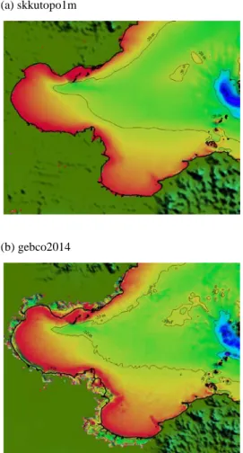
(14) Reports of Research Institute for Applied Mechanics, Kyushu University No.150 March 2016 (a) skkutopo1m. 11. to process large data.. 4.. Discussion. 4.1 Data validation. (b) gebco2014. Fig. 5 Bathymetry of the western Bohai Sea created by using (a) skkutopo1m and (b) gebco2014 datasets. Thin line denotes 20 m isobath contour whereas thick line indicates coastline derived from GSHHS shoreline database18). land portion, the northern Jiangsu coast was not presented correctly, due to the error inherent in SRTM30 topographic data15) used in the datasets. Skkutopo1m and tecs bathymetries (Figs. 3i and 3j), regional products based solely on in-situ sounding data, were found to show similar contour patterns which basically follow features presented in navigational charts. In addition, both datasets do not indicate unrealistic depths indicated in etopo and gebco datasets, e.g., a deep hole exceeding 100 m in the Yangtze Shoal in gebco2014 (Fig.3h). These two datasets therefore seem to represent consistent regional bathymetry in the sense showing generic features properly without having unrealistic extreme values. Difference between skkutopo1m and tecs was found in the representation of small scale features, e.g., radial sand ridges off the Jiangsu coast was not well resolved in the former dataset. Such discrepancy may be ascribed to difference in the number of sounding data available at the time of data compilation, and also to the difference in the computer power. To examine the characteristics of the bathymetric datasets more in detail, enlarged bathymetry maps of four major datasets, etopo1, gebco2014, skkutopo1m and tecs, are shown in Fig. 4 for region off the southwest Korea. It is found that all four dataset show common basic feature that a trench deeper than 60 m transverse the area from southeast to northwest. It was found that generic contour pattern observed in etopo1 (Fig. 4a) were quite similar to those in gebco2014 (Fig. 4b), e.g., distribution of 60 m contour including those bounding deep trenches in the northernmost area which were not observed in skkutopo1m or tecs (Figs. 4c and 4d). Pattern of 40 m contour in the southwestern portion also resembles with each other. On the other hand, gebco2014 seems to represent smallscale features found in the Korean side of the Yellow Sea more in detail. For example, linear sand ridges in the northeastern area were discernible only in gebco2014 and tecs. An isolated island northwest of Cheju Island (Soheuksando), eastern and western sides of which are bounded by trenches deeper than 100 m, seems to have represented in proper size in gebco2014 and tecs. Small-scale features in the southwestern part of Fig. 4 were observed only in gebco2014 (Fig. 4b). Though the feature might be reflecting actual deep and shallow depths sampled from a sequence of submerged valleys observed in this region, it probably requires more sounding data to resolve the feature in more realistic manner. A lattice-like feature ca. 70 m deep found in the northwestern area of etopo1 and gebco2014 (Figs. 4a and 4b) were originated from an inclusion of single-beam sounding data not adopted in tecs (Fig. 4d). Depth contour of tecs, in contrast, does not show detailed structure compared to etopo1 and gebco2014 in this area because there was not enough sounding data available in the mid-Yellow Sea. In etopo1, gebco2014 and tecs, a series of circular ridgeand-hollow features were found at a region west of Cheju Island, which seems to have caused by insufficient sampling interval of the source sounding data compared to the spatial scale of bottom features. This result suggests that the number of sounding data is still insufficient to resolve bottom features at some regions. In summary, it was suggested that tecs dataset provides consistent bathymetry patterns as in skkutopo1m, while the dataset also resolves detailed small-scale features at area where sounding data are densely distributed..

(15) 12. Uehara: East China Sea bathymetric data. Fig. 6 Bathymetric contours (5 m interval) in region west of Cheju Island derived from skkutopo1m dataset (red lines) and from bathymetric chart based on acoustic sounding issued by Korean Institute of Geology, Mining and Materials in 1993 (blue lines), which were overlain by U.K. chart 3480. The location of the area is indicated in the map in the right hand side created from skkutopo1m bathymetry.. 4.2 Spurious coastal features in gebco2014 Though previous analyses have shown that gebco2014 has high potential to represent bottom features in the ECS, its depth value seems to contain systematic error along some coastlines. Fig. 5 compares the depth distribution of the western Bohai Sea derived from skkutopo1m with that from gebco2014. Unlike skkutopo1m (Fig. 5a), sea area presented in gebco2014 bathymetry has extended further landward from the actual position and depths along the inundated coastal zone exceeded 30 m (Fig. 5b), which is a spurious feature because many of the deep areas are supposed to be lowlands such as intertidal zones or shallow salt pans. It is speculated that this spurious feature is related to the specification of gebco bathymetries not using 0 m height (or depth) to avoid problems when connecting land and sea data. Large area without having any height or depth might have produced the spurious values. Fig. 5 shows another issue specific to the ECS where coastline has changed greatly in the past several decades. The coastline around the Yellow River Delta indicated in skkutopo1m (Fig. 5a) and gebco2014 (Fig. 5b) bathymetries resembles with actual coastlines observed in 1960s and 1950s, respectively. The coastline shown in Fig. 5 derived from GSHHS database17) also reflects the status of 1960s. As changes in the coastline have modified the tidal range in the Bohai Sea for more than 20 cm18), it might be necessary to incorporate latest coastlines to the bathymetric dataset when studying resent status of the ECS.. 4.3 Impact of sounding data distribution Red lines indicated in Fig. 6 denote the depth contour of skkutopo1m at the entrance of the Yellow Sea. Comparison. with depth contours derived from more detailed bathymetric chart, shown in blue lines, suggests that a north-south shoal west of Cheju Island was a spurious feature generated by connecting depths on top of some ridges found in elongated ridge-and-swale features aligned in ESE-WNW direction. This example shows that the usage of insufficient number of data compared to the spatial scale of bottom features may give rise to a spurious bathymetry. The distribution of sounding data currently available (Fig. 1) shows that the in-situ data is lacking especially in the central Yellow Sea, the northern Japan Sea and the outer shelf area of the East China Sea. In addition, many depth data indicated in charts covering central Liaodong Gulf and North Korean waters are measured in more than half century ago and needs to be replaced. Additional sounding data are required to improve the quality of the bathymetric data in the ECS.. 5. Summary and conclusion New grid bathymetric data of the ECS has developed, which was found to possess the consistency of overall patterns as in skkutopo1m bathymetry and also was found to resolve some small-scale features as in gebco2014 dataset. Differences in bottom features found in existing bathymetric datasets suggests the importance of choosing appropriate dataset. Aside from the new bathymetry compiled in this study, it might be safe to use skkutopo1m bathymetry or gebco2014 bathymetry (after revising spurious features) for the purpose of a regional study. The current study also has shown that a sufficient number of sounding data compared to the spatial scale of bottom features are necessary to avoid the emergence of spurious bathymetry. Though the situation has improved greatly in the last decade, additional sounding data covering the ECS is necessary to improve the data quality..

(16) Reports of Research Institute for Applied Mechanics, Kyushu University No.150 March 2016. References 1). 2). 3). 4). 5). 6). 7). 8). Uehara, K., Compilation of bathymetric data for the South China Sea 2: High resolution dataset based on multiple sources, Eng. Sci. Rep., Kyushu Univ., 37(2), 12-18, 2016 National Geophysical Data Center, NOAA, Digital relief of the Surface Earth, Data Announcement 88-MGG-02, 1988 (http://ngdc.noaa.gov/mgg/global/etopo5.HTML) National Geophysical Data Center, NOAA, ETOPO2, Global 2 Arc-minute Ocean Depths and Land Elevations, 2001 (supplied in form of CD-ROM) Amante, C., B.W. Eakins, ETOPO1 1 Arc-Minute Global Relief Model: Procedures, Data Sources and Analysis. NOAA Technical Memorandum NESDIS NGDC-24, 2009 (doi:10.7289/V5C8276M, accessed Nov.22, 2015) (http://www.ngdc.noaa.gov/mgg/global/global.html) Smith, W.H.F., D.T. Sandwell, Global Sea Floor Topography from Satellite Altimetry and Ship Depth Soundings, Science, 277(5334), 1956-1962, 1997 National Geophysical Data Center, NOAA, 5-Minute Gridded Global Relief Data Collection (ETOPO5), Data Announcement 93-MGG-01, 1993 (http://www.ngdc.noaa.gov/mgg/fliers/93mgg01.html) National Geophysical Data Center, NOAA, 2-minute Gridded Global Relief Data (ETOPO2v2), 2006 (http://www.ngdc.noaa.gov/mgg/fliers/06mgg01.html) IOC, IHO, and BODC, Centenary Edition of the GEBCO Digital Atlas, published on CD-ROM on behalf of the Intergovernmental Oceanographic Commission and the International Hydrographic Organization as part of the General Bathymetric Chart of the Oceans; British Oceanographic Data Centre, Liverpool, 2003 (http://www.gebco.net/data_and_products/gebco_digital_atlas/). 9). British Oceanographic Data Centre, User guide to the GEBCO One Minute Grid, BODC Document 301381,. 13. 2008 (https://bodc.ac.uk/data/documents/nodb/301381/) 10) British Oceanographic Data Centre, General Bathymetric Chart of the Oceans (GEBCO) The GEBCO_08 Grid (version 20100927), 19pp., 2010 11) British Oceanographic Data Centre, The GEBCO_2014 Grid, BODC Document 301801, 2014 (https://www.bodc.ac.uk/data/documents/nodb/301801/) (http://www.gebco.net/data_and_products/gridded_bathymetry _data/gebco_30_second_grid/) (https://www.bodc.ac.uk/data/online_delivery/gebco/gebco_30_ second_grid/). 12) Choi, B.H., K.O. Kim, H.M. Eum, Digital Bathymetric and Topographic Data for Neighboring Seas of Korea, J. Korean Soc. Coast. Ocean Eng., 14(1), 41-50, 2002 13) Japan Oceanographic Data Center, J-EGG500, JODCExpert Grid data for Geography -500m, 2002 (http://www.jodc.go.jp/data_set/jodc/jegg_intro.html) 14) Marine Information Research Center, Jana Hydrographic Association, JTOPO30v2--30 minutes grid bathymetric data around Japanese waters, 2nd edition, 2011 (http://www.mirc.jha.jp/products/JTOPO30v2/) 15) GLOBE Task Team, The Global Land One-kilometer Base Elevation (GLOBE) Digital Elevation Model, Version 1.0, 1999 (http://www.ngdc.noaa.gov/mgg/topo/globe.html) 16) Becker, J.J. et al., Global Bathymetry and Elevation Data at 30 Arc Seconds Resolution: SRTM30_PLUS, Mar. Geod. 32(4), 355-371, 2009 17) Wessel, P. and W.H.F. Smith, A Global Self-consistent, Hierarchical, High-resolution Shoreline Database, J. Geophys. Res., 101(B4), 8741-8743, 1996 (http://www.ngdc.noaa.gov/mgg/shorelines/gshhs.html) 18) Pelling, H.E., K. Uehara, J.A.M Green, The impact of rapid coastline changes and sea level rise on the tides in the Bohai Sea, China, J. Geophys. Res., 118, 11pp., 2013 (doi:10.1002/jgrc.20258).

(17) Reports of Research Institute for Applied Mechanics, Kyushu University No.150 (14– 24) March 2016. Significant impacts of heterogeneous reactions on the chemico-physical properties of dust particles during severe dust events over East Asia in 2015 Zhe WANG*1, 2, Xiaole PAN*3, Jie LI*1, Zifa WANG*1, Pingqing FU*1, Ting YANG*1, Hiroshi KOBAYASHI*4, Atsushi SHIMIZU*5, Nobuo SUGIMOTO*5, Shigekazu YAMAMOTO*6 and Itsushi UNO*2 E-mail of corresponding author: [email protected] (Received January 29, 2016). Abstract Heterogeneous processes play an important role in changing the chemical, physical, optical, and radiative characters of dust particles at regional and global scales, especially in East Asia, where both the emissions of mineral dust and anthropogenic pollutants are huge. To investigate the chemical and physical impacts of heterogeneous reactions on dust particles, three dust and/or air pollution episodes were observed and simulated in Beijing, China and Fukuoka, Japan during 27 March and 2 April, 2015. The results confirmed that heterogeneous reactions were the major mechanisms producing coarse mode nitrate and sulfate in the presence of dust particles, with the concentrations of coarse mode nitrate reaching 19 μg/m3 in Beijing and 4 μg/m3 in Fukuoka. We also found that heterogeneous processes and subsequent hygroscopic growth significantly changed the mixing state and size of dust particles. As a result of the internal mixing of nitrate, sulfate, and aerosol liquid water, the volume concentration of dust doubled when the relative humidity (RH) was relatively high (> 80%), and the dust particles tended to be spherical when the volume fraction of dust coatings reached 20%. Keywords : Dust, heterogeneous reaction, hygroscopic growth, mixing state, particle size, depolarization, sphericity. 1. Introduction A large amount of mineral dust particles are mobilized into the atmosphere by strong surface winds over arid terrain in Asia, and can be transported long distances (e.g., to the northern Pacific, North America, and even one full circuit around the globe) 1). This enhances the heterogeneous chemistry of the atmosphere 2) , and influences the climate by scattering and absorbing *1 Institute of Atmospheric Physics (IAP), Chinese Academy of Sciences (CAS), Beijing, China *2 Research Institute for Applied Mechanics, Kyushu University, Japan *3 Center for Integrated Atmospheric Research, Kyushu University, Japan *4 University of Yamanashi, Yamanashi, Japan *5 National Institute for Environmental Studies, Tsukuba, Ibaraki, Japan *6 Fukuoka Institute of Health and Environmental Sciences, Fukuoka, Japan. incoming solar radiation 3). Compared with pure secondary anthropogenic sulfate and nitrate, sulfate and nitrate carried on dust can be transported over much longer distances. When aged by water soluble aerosol components during transportation, the size, shape, and hygroscopicity of mineral particles may be altered. As a result, the coated dust particles will change their optical properties, and become more efficient cloud condensation nuclei (CCN), which will consequently change both the direct and indirect climate effects of dust particles at regional and global scales. Calcium (Ca) in Asian dust accounts for 39% of the total of seven crustal elements (Si, Al, Mg, Ca, Na, and K), in contrast with Saharan dust particles where Ca only comprises up to 17% 4). Calcium-rich Asian dust particles readily react with anthropogenic acidic species, such as sulfuric and nitric acid. Meanwhile, dust particles may also directly take up high levels of sulfur dioxide (SO2) and nitrogen dioxide (NO2) 5), leading to the formation of water-soluble sulfate and nitrate in.

(18) Reports of Research Institute for Applied Mechanics, Kyushu University No.150 March 2016 large quantities. Therefore, the mixing of Asian mineral dust with anthropogenic pollutants is a critical issue in understanding the problem of ‘polluted dust’. Beijing, China is very close to the source region of dust particles (about 200 km away), and its surrounding area has a larger emission intensity of anthropogenic pollutants than other regions of China, or even the world. In general, during blowing dust events, a strong northwest wind usually carries dust particles through Beijing quickly and directly, and the concentration of anthropogenic pollutants in Beijing decreases significantly due to the high wind speed and dilution. Therefore, almost no sulfate is formed and nitrate is only formed in small quantities on the surface of dust particles during their transport from source areas to Beijing 6). Transmission electron microscopy (TEM) observations in Beijing have indicated that only 5% are covered by visible coatings in the dust sample 7). However, during 29 March to 1 April of 2015, high concentrations of suspended dust and anthropogenic pollutants were trapped in the Beijing area, which provided a good opportunity to observe and simulate the impacts of heterogeneous reactions on the chemico-physical properties of dust particles. In this study, we used a polarization optical particle counter (POPC) to observe the mixing and sphericity of particles of different sizes in Beijing, China for the first time, and we also made POPC observations in Fukuoka, Japan. Filter samples of PM2.5 (particulate matter [PM] with an aerodynamic diameter less than or equal to 2.5 μm) and PM10 (PM with an aerodynamic diameter less than or equal to 10 μm) were collected twice a day in Beijing and analyzed by ion chromatography (IC). In Fukuoka, a continuous dichotomous aerosol chemical speciation analyzer (ACSA) was used to observe the chemical composition of PM2.5 and PM10. The Nested Air Quality Prediction Modeling System (NAQPMS) was also used to simulate the mixing of dust particles with anthropogenic pollutants. Based on the observations and model results, the impacts of heterogeneous chemical reactions on the chemico-physical properties (e.g., chemical composition, particle size, hygroscopicity, and sphericity) of dust particles during severe dust events over East Asia in 2015 was studied in detail.. 2.. Experimental. 2.1 Observations Online observation of the light-polarization property of single particles was performed using a POPC (YGK. 15. Corp., Yamanashi, Japan) at the Institute of Atmospheric Physics (IAP: 116.4˚E, 39.9˚N), Beijing and Kyushu University (130.5˚E, 33.5˚N), Fukuoka, during the spring of 2015. Beijing is located in the downstream region of dust sources (about 200 km away), while Fukuoka is located more than 1,500 km away from the major dust source regions (Fig. 1). POPCs were previously used successfully for dust monitoring in Korea 8) and Japan 9), however, this is the first time it was used for dust monitoring in China. A POPC measures the intensity of the forward scattering signal and two depolarized components (s-polarized, p-polarized) of the backward scattering signal for each single particle illuminated by a linearly polarized laser at a wavelength of 780 nm 10). The intensity of forward scattering was used to determine the size of individual particles. The depolarization ratio (DR), denoted as the ratio of the intensity of the s-polarized component to the backward scattering signal [S/(S+P)], was an indicator of the non-sphericity of the particle. Supermicron particles with a DR > 0.2 and submicron particles with a DR > 0.5 were regarded as being “non-spherical” (e.g., dust). Supermicron particles with a DR < 0.2 had a spherical structure (e.g., anthropogenic pollutants or sea salt) 10). POPCs have been used to investigate the time-resolved mixing state of mineral dust and anthropogenic aerosols 8, 9) . PM2.5 and PM10 were collected on Teflon filters at the IAP at 12 h intervals from March 27 to April 12, 2015. For the extraction of water-soluble components from the aerosol filter sample (diameter of 2 cm), 10 mL of ultra-pure water was added to the sample vial, and then ion-chromatography (ICS-1600 for anions and ICS-1100 for cations; Thermo Fisher Scientific, Waltham, MA, USA) was used to analyze the aerosol ion concentration. The mass concentrations of anthropogenic aerosols in both PM2.5 and PM10 were concurrently measured using a continuous dichotomous ACSA (ACSA-12, Kimoto Electric Co., Ltd., Osaka, Japan) at 1 h time intervals at Kyushu University, Fukuoka 9). The ACSA-12 determines PM, black carbon (BC), sulfate, and nitrate on the basis of β ray absorption, near-infrared light scattering, a BaSO4-based turbid metric, and a UV spectrophotometric method, respectively, with an uncertainty of ~10% 11). A dual-wavelength (1,064 nm, 532 nm) depolarization Lidar developed by the National Institute for Environmental Studies (NIES) 12) was used to continuously observe aerosols below 6 km at 15 minute intervals at the IAP, Beijing 13). The Lidar employs a flash lamp-pumped Nd:YAG laser with a second.

(19) 16. Wang et al.: Impacts of heterogeneous reactions on the chemico-physical properties of dust particles. harmonics generator. The scattered light is received with a 20 cm Schmidt-Cassegrain telescope, and is then collimated and directed to a dichroic mirror to separate received light at 532 and 1,064 nm. The 1,064 nm signal is detected with an avalanche photodiode (APD). The 532 nm wavelength corresponds to depolarization and the light is directed to a polarizer. The polarization components are detected with two photomultiplier tubes (PMTs). The Fernald inversion method is applied to derive the extinction coefficient with S1 set to 50 sr in the inversion process.. 2.2 Numerical Models The NAQPMS 14) was used to simulate the dust and air pollution processes. The model has been used previously to simulate the heterogeneous reactions occurring on dust and BC 15, 16). NAQPMS was configured with the same horizontal resolution and domain as the Weather Research and Forecasting (WRF) model (Fig. 1), and with 20 vertical layers in a sigma coordinate.. The dust source factor (E) represents the uplifting capability of the land surface, and reflects the impact of land use categories, vegetation fractions, and snow/ice cover on dust fluxes. In the desert, without vegetation and snow cover, dust particles are easily uplifted to the boundary layer, and E is set to 1.0. In contrast, E is set to 0.0 in evergreen forest. ∗ and ∗ are the friction and threshold friction velocities. ∗ is related to soil type, mineral particle size distribution, surface roughness, and soil moisture. RH and RH0 represent relative humidity and its threshold value, respectively. In this study, ∗ was set to 0.45, 0.35, 0.6, and 0.4 m s−1 in the Gobi, China Loess, Hunshandak deserts, and other dust source regions, respectively, while RH0 was set to 40 %, following Li et al. 16). The dust particle size was separated into four size bins covering the range of 0.43–10 μm (0.43–1 μm; 1–2.5 μm; 2.5–5 μm, and 5–10 μm) in diameter. The anthropogenic emissions (e.g., SO2, NOx, NH3, CO, BC, OC, and VOCs) were from the MIX (mosaic Asian anthropogenic emission inventory for Model Inter-Comparison Study [MICS]-Asia and Hemispheric Transport of Air Pollution [HTAP] projects, http://meicmodel.org/dataset-mix.html) with base year 2010 prepared by Li et al. 18). To simulate the mixing of aerosols with pollutant gases, 28 heterogeneous reactions on sulfate, soot, dust and seasalt particles have been included by Li et al. 16). The first-order rate constant (k) of each reaction is calculated by uptake coefficient ( ) and surface area density of particles (A) using the following equation suggested by Jacob 19): (2). Fig.1 Model domain and spatial distributions of dust emissions (unit: ton/km2) during 27 March to 1 April, 2015. The white square and circle indicate the locations of Beijing and Fukuoka, respectively.. where r is the dust particle mean radius, Dg is the gas phase diffusion coefficient, c is the mean molecular speed of the gas,. is the uptake coefficient, and A is. the surface area density of the particles. Among the 28 heterogeneous reactions, the 12 reactions on dust. Dust emissions were computed online using a modified size-segregated dust deflation module 16, 17). The mineral dust emission intensity (F), considering soil categories, vegetation fraction percentages, and snow/ice cover, was determined using the following equation: ∙. ∙. ∙. ∗. 1. ∗ ∗. ∙ 1. ∗ ∗. ∙ 1. (1). where F is the dust flux (kg m−2 s−1). The constant C1 is set to 1.0 × 10−5, and (kg m−3) and g (m2 s−2) are the air density and acceleration due to gravity, respectively.. particles and their uptake coefficients are listed in Table 1. The WRF (version 3.7.1) model was used to investigate the detailed meteorological conditions over East Asia. The model was configured with a horizontal resolution of 45 km (Fig. 1) and 30 vertical layers. National Centers for Environmental Prediction (NCEP) operational global final analysis (FNL) data (1° × 1°, http://dss.ucar.edu/datasets/ds083.2/) were used as the initial and boundary conditions..

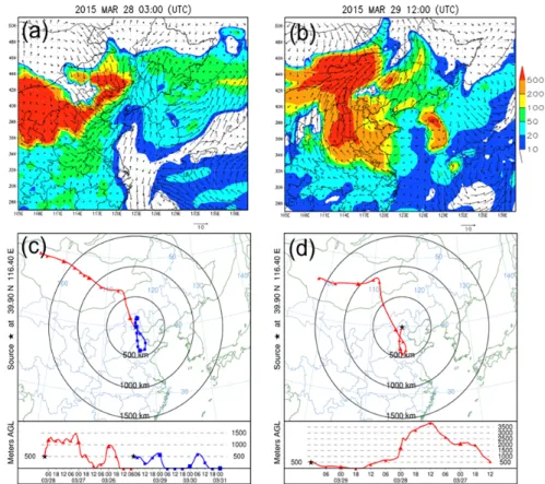
(20) Reports of Research Institute for Applied Mechanics, Kyushu University No.150 March 2016. 17. Table 1. Heterogeneous reactions on dust particles and reactive uptake coefficients Heterogeneous Reactions O3 +dust→products HNO3+dust→NO. 2.7 × 10-5 1. RH. c RH 1 1. c. RH. 0.018 c. NO2 +dust→0.5HONO+0.5HNO3. 2.1 × 10-6. NO3 +dust→HNO3. 1.0 × 10-3. N2 O5 +dust→2HNO3. 3.0 × 10-2. OH+dust→products. 1.0 × 10-1. HO2 +dust→0.5H2 O2. 2.0 × 10-1. H2 O2 +dust→products. 12 × RH-2 - 5.95 × RH + 4.08. SO2 +dust→SO. 1.0 × 10-4. CH3 COOH+dust→products. 1.0 × 10-3. CH3 OH+dust→products. 1.0 × 10-5. HCHO+dust→products. 1.0 × 10-5. 8. The back and forward trajectories of air masses are calculated by a Hybrid Single-Particle Lagrangian Integrated Trajectory (HYSPLIT; version 4) model (http://ready.arl.noaa.gov/HYSPLIT.php) during the dust period based on NCEP GDAS global assimilation data (ftp://arlftp.arlhq.noaa.gov/pub/archives/gdas0p5) with 0.5 degree resolution every 3 hours.. 3.. Results and Discussion. 3.1 The Dust and Air Pollution Episodes and Model Evaluation in Beijing Region Three high PM concentration episodes with meteorological parameters were well observed and simulated in Beijing during March 27 to April 1, 2015, as shown in Fig. 2. PM2.5 was observed by tapered element oscillating microbalance (TEOM), while PM2.5-5 (PM with diameter larger than 2.5 μm yet less than 5 μm) and PM5-10 (PM with diameter larger than 5 μm yet less than 10 μm) were constructed by POPC using a density of 1.8 g/cm3. Comparisons of the observed and simulated time series of meteorological parameters (wind vector, wind speed and RH) in Fig. 2 (a–c) also indicated that the model simulation showed a good consistency with observations. The first high PM concentration episode is classified as an anthropogenic air pollution episode on March 27 (Episode A). During this episode, wind speed was less than 5 m/s, and wind direction was south (Fig. 2a and 2b), which is the typical meteorological condition for heavy air pollution processes in Beijing. Fine particles (PM2.5) was dominate with a concentration larger than 100 μg/m3 (Fig. 2d), while PM2.5-5 and PM5-10 concentrations were both less than 50 μg/m3 (Fig. 2e and. Fig.2 Time series of observed and simulated meteorological parameters (a, wind vector; b, wind speed; c, relative humidity) and particulate matter (PM) (d, PM2.5; e, PM2.5-5; f, PM5-10) concentrations in Beijing. Black dashed lines in (d–f) indicate simulated dust PM, while blue lines indicate total PM (= anthropogenic + dust). 2f). From the simulated anthropogenic PM and dust concentration, it is clearly shown that PM2.5 was mostly anthropogenic particles, while PM2.5-5 and PM5-10 were mostly dust. The second high PM concentration episode is a pure dust episode, on March 28 (Episode B). This pure dust episode is a blowing dust process with a strong northwest wind higher than 10 m/s, lasting for only about 5 hours. During this episode, the PM2.5 concentration was less than 103 μg/m3; however, PM2.5-5 and PM5-10 concentrations increased significantly with maximum values of 382 μg/m3 and 314 μg/m3, respectively. The third high PM concentration episode is a mineral dust mixing with anthropogenic air pollution episode.

(21) 18. Wang et al.: Impacts of heterogeneous reactions on the chemico-physical properties of dust particles. during March 29 to March 31 (Episode C). This mixing dust episode was a floating dust process with a weaker south wind less than 5 m/s, different from typical dust processes with a strong north wind. During this episode, the PM2.5 concentration increased gradually to a maximum of about 200 μg/m3, while the PM2.5-5 and PM5-10 concentration decreased gradually from a maximum of about 200 μg/m3 and 150 μg/m3, and dust particles were mixing with anthropogenic pollutants. Figure 3a and 3b shows the dust transport pattern on March 28 03:00 UTC (Episode B) and March 29 12:00 UTC (Episode C), while Figs 3c and 3d are backward and forward trajectory from Beijing ending at the same. time with Fig. 3a and 3b, respectively. Dust particles were mainly emitted from Mongolia and Inner Mongolia province of China (Fig. 1), and arrived at Beijing rapidly (within half a day) following the strong northwest wind (> 10 m/s) on March 28 (Fig. 3a and 3c), and stayed in Beijing for only about 5 hours (Episode B). Then, the dust was quickly transported to about 500 km southeast of Beijing (i.e., Hebei and Shandong province). However, the dust cloud once swept out from the Beijing region, and was transported back to Beijing again under the south wind over North China on March 29 (Fig. 3b and 3d); the high PM concentration in Beijing then continued for about 2 days (Episode C) (Fig. 2).. Fig.3 Horizontal distribution of dust concentration (unit: μg/m3) and wind vector (unit: m/s) on March 28 03:00 UTC (a) and 29 12:00 UTC (b). (c) and (d) are backward (Red) and forward (blue) trajectory from Beijing at the same time with (a) and (b). Figure 4a and 4c present time-height indications of the extinction coefficients of non-spherical aerosols (mostly mineral dust) and spherical aerosols (mostly anthropogenic particles) derived from Lidar measurements using a method based on the assumption of external mixing between two types of particles with different particle DRs 12). The NAQPMS model simulated results are also shown in Fig. 4b and 4d. The vertical distributions of aerosol during the three episodes were quite different. On March 27 (Episode A), the aerosol extinction coefficient was mainly caused by the. anthropogenic aerosol, and it reached heights less than 1,500 m. However, on March 28 (Episode B), the dust extinction coefficient was dominant, and it reached as high as 4 km, and lasted for about 5 hours. During March 29 to 31 (Episode C), both dust and anthropogenic aerosols reached about 2 km, less than the height during Episode B, indicating that only the dust in the lower layer went back. The model results were in close agreement with the Lidar retrieval for both the timing and vertical distribution of high concentration events..

(22) Reports of Research Institute for Applied Mechanics, Kyushu University No.150 March 2016. 19. Fig.5 Time series of PM10 concentration (a), volume size distributions (b) and mode depolarization ratios (MDRs) (c) of ambient particles at Beijing.. Fig.4 Lidar-observed (a, c) and model-simulated (b, d) time-height indications of anthropogenic (a, b) and dust (c, d) extinction coefficients. Time series of PM10 concentration, volume size distributions and mode DRs of ambient particles observed by POPC at Beijing are shown in Fig. 5, and the PM10 concentration observed by TEOM is also shown in Fig. 5a. The constructed PM10 mass concentration by POPC is also consistent with the online measurement of PM10 by TEOM. From Fig. 5b, we can see that the volume concentrations of ambient particles generally had two significant peaks in the submicron and/or coarse mode size ranges, representing anthropogenic particles and mineral dust particles. During Episode A (March 27) submicron particles had a larger volume concentration; while coarse mode particles were dominate during Episode B (March 28); however, during Episode C (from March 29 to March 30), coarse mode particles decreased gradually and mixed with the increasing submicron particles. To reveal the sphericity of coarse and submicron particles, the DRs of particles at each size range as a function of time are shown in Fig. 5c. Because the DR value of any size range particles was always characterized by a skewness of the distribution, a mode DR (MDR) value was used to represent their typical depolarization property. As shown in Fig. 5c, particles with diameter larger than 2 μm had larger DR values, indicating that they were more non-spherical, and DR values were higher during dust. periods (Episodes B and C) compared to non-dust periods.. 3.2 Transport of Dust and Pollution to Fukuoka Figure 6 compares the observed and simulated time series of PM concentrations with different bin size at Fukuoka. In general, PM concentrations were underestimated by the model during March 27 to 29; however, the model captured the peak of PM concentration on March 30 and showed a similar magnitude ( about 40 μg/m3 for PM2.5 and PM2.5-5, 60 μg/m3 for PM5-10). Similar to Beijing, PM2.5 in Fukuoka was mostly anthropogenic particles, while almost all the PM2.5-5 and PM5-10 were mineral dust. Similar to Fig. 5, POPC observations at Fukuoka are shown in Fig. 6 (d–f). The constructed PM10 by POPC are also consistent with the PM10 observed by ACSA (Fig. 6d). The PM10 concentration of Fukuoka reached about 107 μg/m3 in March 30, and consisted mostly of coarse particles with diameter larger than 2 μm (Fig. 6e), but with more submicron particles compared to the pure dust Episode B of Beijing. As shown in Fig. 6f, on March 30, DR values of the particles with diameters larger than 2 μm increased significantly, as they were affected by non-spherical dust particles, while DR values of submicron particles were still low. By comparison of the Fukuoka dust episode with Episode B of Beijing, it is indicated that the dust particles were mixed with anthropogenic aerosols gradually during the transportation from China to Japan..

(23) 20. Wang et al.: Impacts of heterogeneous reactions on the chemico-physical properties of dust particles. Fig.7 Backward trajectory from Fukuoka ending on March 30 at 12:00 UTC.. 3.3 Impacts of Heterogeneous Reactions on Aerosol Mixing State and Chemical Composition. Fig.6 Time series of observed and simulated PM concentrations at Fukuoka: (a) PM2.5; (b) PM2.5-5; (c) PM5-10; and PM10 concentration (d), volume size distributions (e) and MDRs (f) of ambient particles measured by a polarization optical particle counter (POPC) at Fukuoka. Black dashed lines in (a–c) indicate simulated dust PM, while blue lines indicate total PM. Figure 7 presents the backward trajectory from Fukuoka ending on March 30 at 12:00 UTC. From the trajectory plot, it is shown that the high-concentration dust on March 30 was transported from the northeast part of the Beijing-Tianjin-Hebei area from March 28, at the same time as with Episode B in Beijing, which indicates that the dust of Fukuoka on March 30, and of Episode B in Beijing, were the same dust plume. However, different to the trajectory in Fig. 3c and 3d, this trajectory went straight to Kyushu Island after it passed north Hebei without turning back, because the heights of air masses along the trajectories in Figs. 3 and 7 were different on March 28. The air mass on March 28 in Fig. 3 was in the atmospheric boundary layer ( < 1,500 m), while the air mass on March 28 in Fig. 7 was in the middle troposphere (about 5,000 m).. To identify the aerosol mixing state of the different episodes, volume concentrations as a function of particle size and DR for anthropogenic aerosols (Episode A), mineral dust (Episode B), and mixing particles (Episode C) in Beijing are shown in Fig. 8a, 8b and 8c, respectively; concentrations during the dust episode in Fukuoka are also shown. It can be seen that anthropogenic aerosols were mostly in the submicron range, with DR values < 0.2 (Fig. 8a). Mineral dust had a larger diameter (Dp > 3 μm) and a non-spherical morphology associated with larger DR values (0.2–0.4); the fraction of calcium ions mass concentration relative to the total mass concentration of sulfate, nitrate, ammonium and calcium reached 40% in both PM2.5 and PM10 (Fig. 8b). During Episode C (Fig. 8c), both anthropogenic aerosols with small diameters and DR values and dust particles with large diameters and DR values shown to be present in a large volume, indicating they were mixing together during this period. The mass fraction of calcium ions was only 3% in PM2.5 and 11% in PM10 , indicating that the mineral dust decreased significantly compared to Episode B, because of deposition and diffusion of dust particles and formation of secondary inorganic aerosols during the transportation. From Episode B to Episode C, the fine mode calcium fraction decreased, from 40% to 3%, more rapidly than for the coarse mode (from 40% to 11%), because of more anthropogenic secondary inorganic aerosols formation in fine mode than in coarse mode. As the dust of Fukuoka on March 30 was transported from Episode B of the Beijing region, by comparison of Fig. 8b and 8d, it is clearly seen that there were more fine mode.

(24) Reports of Research Institute for Applied Mechanics, Kyushu University No.150 March 2016. 21. Fig.8 Volume concentrations as a function of particle size and DR during (a) anthropogenic pollution, (b) mineral dust, (c) mixed dust episode in Beijing, and (d) mixed dust episode in Fukuoka. The red, blue, green, and yellow colors in the pie charts indicate the mass fraction of sulfate, nitrate, ammonium and calcium ions in PM2.5 and PM10. particles, and DR became smaller in Fukuoka than in Beijing, which indicated that the dust particles were mixed with anthropogenic aerosols during the transportation. Figure 9 shows the observed and simulated fine and coarse mode aerosol chemical composition in Beijing. The simulated fine mode concentrations of ammonium, nitrate and sulfate, with maximum values of 27 μg/m3, 61 μg/m3 and 44 μg/m3, respectively, were in good agreement with the observed fine mode concentrations. The simulated fine mode concentrations of ammonium, nitrate and sulfate were mainly due to anthropogenic pollutants, with no dust ammonium and less than 5 μg/m3 of dust nitrate and sulfate. The simulated coarse mode concentrations of calcium, nitrate and sulfate had maximum values of 9 μg/m3, 19 μg/m3 and 7 μg/m3, respectively, and were products of heterogeneous reactions on dust; this is also in good agreement with observed coarse mode concentrations. Furthermore, both observation and model results showed that the coarse mode concentrations of nitrate, sulfate and calcium ions were low during the air pollution episode, but high during the mixing dust episode; meanwhile, the coarse mode ammonium concentration was always low. These. results confirmed that heterogeneous reactions were major sources of coarse mode nitrate and sulfate in the presence of dust particles.. Fig.9 Observed and simulated fine and coarse mode chemical composition in Beijing..

(25) 22. Wang et al.: Impacts of heterogeneous reactions on the chemico-physical properties of dust particles. Observed and simulated coarse mode nitrate levels in Fukuoka are also shown in Fig. 10. Observed coarse mode nitrate in Fukuoka was usually less than 1 μg/m3, but increased significantly and reached 4 μg/m3 during the dust period. The model generally captured this variation and showed a similar peak magnitude. The simulated coarse mode nitrate was nearly zero during the non-dust period, because NAQPMS supposed that all the anthropogenic nitrate was in the fine mode.. series of the volume concentration (a) and volume fraction (b) of dust, secondary inorganic aerosol and aerosol water content, and also (c) the time series of DR. The maximum volume of nitrate and sulfate coatings reached about 10 ppbV and 20% of the dry coated dust particles; meanwhile, the aerosol liquid water reached 10 to 20 ppbV due to hygroscopic growth (Fig. 11a), and made the dust particles become larger by a factor of 2 on March 31 and April 1 (Fig. 11b) when the RH was relatively high (> 80 %, Fig. 2e). As a result of internal mixing of nitrate, sulfate and aerosol liquid water, the DR decreased significantly (Fig. 11c), and the dust particles became spherical (DR < 0.1) when the volume fraction of dust coatings reached to 20% (Fig. 11d). The relationship between aerosol DR and volume percentage of coatings to coated dust particles can be expressed as (Fig. 11d): .. DR. Fig.10 Observed and simulated coarse mode nitrate in Fukuoka.. 3.4 Impacts of internal mixing on hygroscopic growth and sphericity of dust particles Since the heterogeneous reactions had changed the chemical composition of dust particles, the secondary inorganic coatings and their hygroscopic growth significantly changed the mixing state, the size and the sphericity of dust particles. Figure 11 shows the time. (3) 0.12 where is the total volume of coatings, is the volume of secondary aerosol coatings on the dust surface, and is the volume of aerosol liquid water content due to the hygroscopic growth of .. is the volume of coated dust particles. is the volume of dust cores. The volume of aerosol liquid water content was calculated based on Shamjad et al. 20): (4) where. ∑. /∑. is the hygroscopicity of. Fig.11 Time series of (a) volume concentration and (b) volume fraction of Nested Air Quality Prediction Modeling System (NAQPMS) simulated dust, secondary inorganic aerosol and aerosol water content; (c) time series of Lidar-observed DR averaged between 60 m and 200 m and (d) relationship of Lidar-observed DR and NAQPMS-simulated volume percentage of coatings..

九州大学応用力学研究所 Reports No.150（Mar. 2016）

九州大学応用力学研究所 Reports　No.150（Mar. 2016）