Acceleration Methods and Discrete Soliton
Equations
(
加速法と離散型ソリトン方程式
)
Atsushi NAGAI (永井敦) \dagger
Junkichi
SATSUMA
(薩摩順吉)Department
of
Mathematical Sciences, Universityof
Tokyo\dagger $\mathrm{e}$-mail: [email protected]
\S 1
IntroductionIntegrable discretizationofsolitonequations hasbeenin progresssince $1970’ \mathrm{s}^{1}$
.
Recentlydiscretesoliton equations have attracted attention in other fields such as engineering. For example, finite,
nonperiodic Toda equation appears in the field ofmatrixeigenvalue algorithm $[2, 3]$
.
The discrete(potential) $\mathrm{K}\mathrm{d}\mathrm{V}$equation is nothing but one
of the most popular convergence accelerationschemes,
the $\epsilon$-algorithm [4].
Our main interest in this paper is on the convergence acceleration algorithms. Let $\{S_{m}\}$ be a
sequence of numbers which converges to $S_{\infty}$
.
In order to find $S_{\infty}$, direct calculation often requiresalarge amount ofdata. Sequences
$S_{m}$ $=$ $1- \frac{1}{2}+\frac{1}{3}-\cdots+\frac{(-1)^{m}}{m+1}$, (1) $S_{m}$ $=$ $1+ \frac{1}{2^{2}}+\frac{1}{3^{2}}+\cdots+\frac{1}{(m+1)^{2}}$ (2)
are typical examples. Beside these simple cases, one has often to deal with slowly convergent
sequences in the fieldof numerical analysis, appliedmathematics, and engineering. Insuch cases we
transform the original sequence $\{S_{m}\}$ into another sequence $\{T_{m}\}$ instead ofcalculating directly. If
$\{T_{m}\}$ converges to $S_{\infty}$ faster than $\{S_{m}\}$, that is
$\lim_{marrow\infty}\frac{T_{m}-S_{\infty}}{S_{m}-S_{\infty}}=0$,
(3)
we say that the transformation $T$ : $\{S_{m}\}arrow\{T_{m}\}$ accelerates the convergence of the sequence
$\{S_{m}\}$
.
We now have various kinds of convergence acceleration algorithms such as $\epsilon$-algorithm [5],$\eta$-algorithm [6], $\rho$-algorithm $[7, 8]$,
$\mathrm{B}\mathrm{S}$-algorithm [9], Levin’s $t-,$ $u-$, and $v$-transformation [10],
and $\theta$-algorithm [11].
The main purpose of this paper is to study acceleration methods from a different aspect, that
is, the soliton theory. In \S 2, we introduce Bauer’s $\eta$-algorithm and show its equivalence with the
discrete $\mathrm{K}\mathrm{d}\mathrm{V}$ equation [1]. In \S 3, we look over the result by Papageorgiou et al., the equivalence
between Wynn’s $\epsilon$-algorithm and the discrete potential
$\mathrm{K}\mathrm{d}\mathrm{V}$ equation. In \S 4, we introduce a
different type of algorithm, Wynn’s $\rho$-algorithm. In spite of its similarity with the
$\epsilon$-algorithm,
it possesses noticeably different characteristics not only as a convergence accelerator but also as a
discrete soliton equation. When we respect the $\rho$-algorithm as atwo-variable difference equation,
its solution is represented by double Casorati determinant. We show in
\S 5
that this fact is quitenatural if we discuss the $\rho$-algorithm in relation with Thiele’s interpolation formula [7]. We also
present the Thiele’s $\rho$-algorithm, which is onegeneralization of the $\rho$-algorithm, and compareits
performance with theoriginal$\rho$-algorithm. In \S 6, we considerthe “PGR algorithms”, which arethe
most generalized rhombus algorithms satisfying the singularity confinement condition. Concluding
remarks are given in \S 7.
\S 2
The $\eta$-algorithm
In this section we show that Bauer’s $\eta-\mathrm{a}_{0}\mathrm{r}\mathrm{i}\mathrm{t}\mathrm{h}\mathrm{m}[6]$, which is one of the famous convergence
acceleration algorithms, is equivalent to the discrete $\mathrm{K}\mathrm{d}\mathrm{V}$ equation. The
$\eta$-algorithm involves a
two-dimensional array called the $\eta$-table (Figure 1). The table is constructed from its first two
columns. Let initial values $\eta_{0}^{(m)}$ and $\eta_{1}^{(m)}$ be
$(m)$ $(m)$
$\eta_{0}$ $=\infty,$ $\eta_{1}$ $=c_{m}\equiv\Delta S_{m-1},$ $(m=0,1,2, \ldots),$ $S_{-1}\equiv 0$, (4)
where $\Delta$ is the forward difference operator givenby $\Delta a_{k}=a_{k+1}-a_{k}$
.
Then all the other elementsare calculated from the followingrecurrence relations called the $\eta$-algorithm;
$\{$
$\eta_{21^{+}}^{(m)}n+\eta_{2}^{(}nm)$ $=$ $\eta_{2n}^{\langle 1)}+m+\eta 2n(m+1)-1$
$\frac{1}{(m)}+\frac{1}{(m)}$ $=$ $\frac{1}{(m+1)}+\frac{1}{(m+1)}$
(rhombus rules).
$\eta_{2n+2}$ $\eta_{2n+1}$ $\eta_{2n+1}$ $\eta_{2n}$
(5)
Equation (5) defines a transformation of a given series $c_{m}=\eta_{1}^{(m)},$$m=0,1,2,$
$\ldots$ to a new series
$c_{n}’=\eta_{n},$$n(\mathrm{O})=1,2,$ $\ldots$ such that $\sum_{n=1^{C}n}^{\infty}$
$\langle 0)$ $\eta_{1}$
$(\infty=)\eta_{0}\langle 1)$ $\eta_{2}^{\langle 0)}$
(1) $(0)$
$\eta_{1}$ $\eta_{3}$
$(\infty=)\eta_{0}(2\rangle$ $\eta_{2}^{\{1)}$ $\eta_{4}^{(0)}$
$\langle$2) (1) $(0)$
$\eta_{1}$ $\eta_{3}$ $\eta_{5}$
$(\infty=)\eta_{0^{3}}\mathrm{t})$ $\eta_{2}^{(2)}$ $\eta_{4}^{\langle 1)}$
.
$\cdot$.
...
$\eta_{1}^{(3)}$ $\eta_{3}^{\{2)}$
.
$\cdot$.
$(\infty=)\eta 0(4)$ $\eta_{2}^{\langle 3)}$
.
$\cdot$.
:.
$\eta_{1}^{(4)}$..
$\cdot$
:
Figure 1: The $\eta$-table.
As a simple example we consider a slowly convergent series (1) and construct the $\eta$-table. We
see from Figure 2 that the transformed series
$1- \frac{1}{3}+\frac{1}{30}-\frac{1}{130}+\frac{1}{975}-\frac{1}{4725}+\cdots$
converges more rapidly to log2 than the original series. While the sum of the first seven terms of
the original series gives 0.7595$\cdots$, that of the corresponding seven terms of the transformed series
does 0.693152$\cdots$
.
1 $\infty$ $-1/3$ $-1/2$ 1/30 $\infty$ 1/5 -1/130 1/3 -1/105 1/975 $\infty$ $-1/7$ 1/350 -1/4725 $-1/4$ 1/252 -1/4100 1/32508 $\infty$ 1/9 -1/738 1/15867 1/5 -1/495 1/12505 $\infty$ $-1/11$ 1/1342 $-1/6$ 1/858 $\infty$ 1/13 1/7$\langle m)$
The quantities $\eta_{n}$ are given by the followingratios of Hankel determinants;
$\eta_{2n+1}^{(m})$ $=$ $\frac{|\begin{array}{lll}c_{m} \cdots c_{m+n}| |c_{m+n} \cdots c_{m+2n}\end{array}|\cdot|\begin{array}{lll}c_{m+1} \cdots c_{m+n}| |c_{m+n} \cdots c_{m+2}n-1\end{array}|}{|\begin{array}{lll}\Delta c_{m} \cdots \Delta c_{m}+n-1| |\Delta c_{m}+n-1 \cdots \Delta c_{m+2}n-2\end{array}|\cdot|\begin{array}{lll}\Delta c_{m+1} \cdots \triangle c_{m+n}| |\Delta c_{m+n} \cdots \Delta c_{m+2}n-1\end{array}|}$ , (6)
$\eta_{2n+2}^{\mathrm{t}^{m)}}$
.
$=$ $\frac{|\begin{array}{lll}c_{m} \cdots c_{m+n}| |c_{m+n} \cdots c_{m+2n}\end{array}|\cdot|\begin{array}{lll}c_{m+1} \cdots c_{m+n+1}| |c_{m+n+1} \cdots c_{m+2n}+1\end{array}|}{|\begin{array}{lll}\Delta c_{m} \cdots \Delta c_{m+n}\vdots |\Delta c_{m+n} \cdots \triangle c_{m+2n}\end{array}|\cdot|\begin{array}{lll}\Delta c_{m+1} \cdots \Delta c_{m+n}\vdots \vdots\triangle c_{m+n} \cdots \Delta c_{m+2}n-1\end{array}|}$
.
(7)If we introduce dependent variabletransformations,
$x_{2n}^{\mathrm{t}^{m})}= \frac{1}{(m)},$ $X_{2n-}=\eta^{(}(m)12nm\rangle-1$ (8)
$\eta_{2n}$
the $\eta$-algorithm (5) is rewritten as
$X^{\mathrm{t}^{m)}}-^{x^{(1}}n+1n-1m+)= \frac{1}{X_{n}^{(+1)}m}-\frac{1}{X_{n}^{(m)}}$, (9)
which is the Hirota’s discrete $\mathrm{K}\mathrm{d}\mathrm{V}$equation [1].
\S 3
The $\epsilon$-algorithm
In this section, following the result by Papageorgiou et al., we briefly review the equivalence
the discrete potential $\mathrm{K}\mathrm{d}\mathrm{V}$ equation and the $\epsilon$-algorithm, which originates with Shanks [13] and
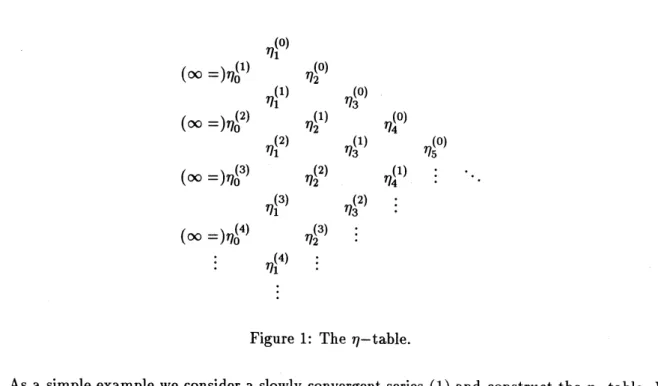
Wynn [5]. The algorithm involves a two-dimensional array called the $\epsilon$-table (Figure 3). Define
$\epsilon_{0}^{(m)}$ and $\epsilon_{1}^{(m)}$ by
$\epsilon_{0}^{(m)}=0,$ $\epsilon_{1}^{(m)}=S_{m}(m=0,1,2, \ldots)$
.
(10)Then all the other quantities obey the following rhombus rule;
$\epsilon_{1}^{(0)}$
$(0=)\epsilon_{0}^{(1)}$ $\epsilon_{2}^{(0)}$ $\epsilon_{1}^{(1)}$ $\epsilon_{3}^{(0)}$
$(0=)\epsilon_{0}^{(2)}$ $\epsilon_{2}^{(1\rangle}$ $\epsilon_{4}^{(0)}$ $\epsilon_{1}^{(2)}$ $\epsilon_{3}^{(1)}$ $\epsilon_{5}^{(0)}$
$(0=)\epsilon_{0}^{(3)}$ $\epsilon_{2}^{\langle 2)}$ $\epsilon_{4}^{(1)}$
.
$\cdot$.
...
$\epsilon_{1}^{\langle 3)}$ $\epsilon_{3}^{(2)}$..
$\cdot$ $(0=)\epsilon_{0}^{(4)}$ $\epsilon_{2}^{(3)}$...
.
$\cdot$.
$\epsilon_{1}^{(4)}$...
$\dot{i}$Figure 3: The $\epsilon$-table
$(m)$
According as $n$ becomes large, $\epsilon_{2n+1}$ converges more rapidly to $S_{\infty}$ as $marrow\infty$
.
On the other hand,$\epsilon_{2n}^{(m)}$ diverges as $marrow\infty$
.
It has been shown that the $\epsilon$-algorithm (11) is regarded as the discrete potential $\mathrm{K}\mathrm{d}\mathrm{V}$
equa-$(m)$
tion [14]. The quantities $\epsilon_{n}$ are also given by the following ratios of Hankel determinants;
$\epsilon_{2n+1}^{(m)}$
$=$ $\frac{|\begin{array}{llll}S_{m} S_{m+1} \cdots S_{m+n}S_{m+1} S_{m+2} \cdots S_{m+n+1}\vdots \vdots \vdots S_{m+n} S_{m+n+1} \cdots S_{m+2n}\end{array}|}{|\begin{array}{llll}\Delta^{2}S_{m} \Delta^{2}S_{m+1} \cdots \Delta^{2}Sm+n-1\Delta^{2}S_{m+1} \Delta^{2}S_{m+2} \cdots \Delta^{2}S_{m+n}| | |\Delta^{2}Sm+n-1 \triangle^{2}S_{m+n} \cdots \triangle^{2}Sm+2n-2\end{array}|}$ , (12)
$\epsilon_{2n+2}^{(m)}$
$=$ $\frac{|\begin{array}{llll}\Delta^{3}S_{m} \Delta^{3}S_{m+1} \cdots \triangle^{3}Sm+n-1\Delta^{3}S_{m+1} \Delta^{3}S_{m+2} \cdots \triangle^{3}S_{m+n}| | |\Delta^{3}S_{m+n}-1 \Delta^{3}S_{m+n} \cdots \Delta^{3}Sm+2n-2\end{array}|}{|\begin{array}{llll}\Delta S_{m} \Delta S_{m+1} \cdots \triangle S_{m+n}\Delta S_{m+1} \Delta S_{m+2} \cdots \Delta S_{m+n}+1| | |\Delta S_{m+n} \Delta S_{m+n}+1 \cdots \Delta S_{m+2n}\end{array}|}$
.
(13)Equation (12) is called the Shanks transformation [13]. Substitution of $n=1$ in eq. (12) gives the
We have so far observed that the $\eta$-and the$\epsilon$-algorithms areinterpretedas the discrete $\mathrm{K}\mathrm{d}\mathrm{V}$
and the discrete potential $\mathrm{K}\mathrm{d}\mathrm{V}$ equations, respectively. Therefore, these two algorithms are the
same in their performance as convergence acceleration algorithms. This equivalence can also be
understood from the fact [6] that the quantities $\eta_{n}^{\langle m)}$
and $\epsilon_{n}^{(m)}$
arerelated by
$\eta_{2n}^{(m)}=\epsilon_{2n+-}^{\mathrm{t}^{m}1}-1)-\epsilon(m)2n1’\eta_{2n+1}^{\mathrm{t}^{m}})=\epsilon_{2+2n+}^{(m)(m-1)}n1^{-}\mathit{6}1$
.
(14)\S 4
The $\rho$-algorithmThe $\rho$-algorithm is traced back to Thiele’s rational interpolation [7]. It was first used as a
convergence accelerator by Wynn [8]. Theinitial values ofthe algorithm are givenby
$\rho_{0}^{(m)}=0,$ $\rho_{1}^{(m)}=S_{m}(m=0,1,2, \ldots)$, (15)
and all the other elements fulfill the following rhombusrule;
$(\rho_{n+}^{\mathrm{t}}m)1^{-\rho n}(m+1))(\rho(m+1)-1n-\rho^{\mathrm{t}m)}n)=n$
.
(16)The $\rho$-algorithm is almost the same as the
$\epsilon$-algorithm except that “1” in the right hand side of
eq. (11) is replaced by “
$n$” in eq. (16). This slight change, however, yields considerable differences
in various aspects between these two algorithms.
The first difference is in their performance. As one can find in ref. [15], the $\epsilon$-algorithm
ac-celerates exponentially or alternatively decaying sequences, while the $\rho$-algorithm does rationally
decayingsequences.
The second differenceis in theirdeterminant expressions. The quantities$\epsilon_{n}$ are givenbyratios
$(m)$
of Hankel determinants,while the quantities $\rho_{n}^{(m)}$ are given by [7]
$\rho_{n}^{(m)}=(-1)^{[\frac{n-1}{2}}]_{\frac{\tilde{\tau}_{n}^{(m)}}{\tau_{n}^{(m)}}}$, (17)
where $[x]$ stands for the greatest integer less than or equal to $x$
.
Moreover, the functions $\tau_{n}^{(m)}$ and$\tilde{\tau}_{n}^{(m)}$
are expressed as the following double Casorati determinants;
$\tau_{n}^{\langle m)}$ $=$ $\{$ $u^{(m)}(k;k)$ $n=2k$, $u^{(m)}(k+1;k)$ $n=2k+1$, (18) $\tilde{\tau}_{n}^{(m)}$ $=$ $\{$ $u^{(m\rangle}(k+1;k-1)$ $n=2k$, $u^{(m)}(k;k+1)$ $n=2k+1$, (19)
where
$u^{\langle m)}(p;q)=\det$
$1$ $1$ $|$ $S_{m+1}$ $(m+1)S_{m}+1$ $(m+1)^{q}-1s_{m}+1$ $1$ $S_{m}.\cdot$.
$m.\cdot.S_{m}$ $.\cdot...\cdot..\cdot$ $(m+p+q-1^{\cdot}.)^{q}-Sm^{q-}.1sm_{1}m+p+q-1]$.
(20) $1$ 1 $1|S_{m+\mathrm{P}+q-}1$ $(m+p+q-1)Sm+p+q-1$We remark that a pair of functions $\tau_{n}^{\langle m)}$
and $\tilde{\tau}_{n}^{(m)}$
given by $\mathrm{e}\mathrm{q}\mathrm{s}$
.
(18) and (19) satisfy bilinearequations,
$\mathcal{T}\mathcal{T}_{n}--n+11nn\langle m)(m+1)\mathrm{t}m)_{\tilde{\mathcal{T}}_{n}+=}(\tau+m1)\mathrm{t}\tau)m+1\tilde{\mathcal{T}}n(m\rangle 0$ , (21)
$\tau_{n-}^{\langle m+}\tilde{\tau}11)(m)n+1^{+n}\tau^{(m)_{\tilde{\tau}-}}n+1n-1n\mathrm{t}^{m+}1)\tau^{\mathrm{t}m)_{\tau}\langle 1)}nm+=0$, (22)
which are consideredto be theJacobi and the Pl\"uckeridentities for determinants, respectively.
\S 5
ReciprocalDifferences
andThiele’s
$\rho$-algorithm
In this section we extend the $\rho$-algorithm from the viewpoint of the $\tau$ function and compare
its performance with the original $\rho$-algorithm (16). Before touching upon the extended version
of the $\rho$-algorithm, we review Thiele’s interpolation [7], which makes it natural that quantities
$(m)$
$\rho_{n}$ are given by ratios of double Casorati determinants. Let the values of an unknown function $f(x)$ be given for the values $x_{0},$$x_{1,n}\ldots,x$, no two ofwhich are equal. Then reciprocal differences
$\rho i(x_{kk}X+1\ldots xk+i-1)$ are defined by
$\rho_{1}(x\mathrm{o})$ $=$ $f(X_{0})$, (23)
$\rho_{2}(_{X_{0}}x_{1})$ $=$ $\frac{x_{0}-x1}{\rho_{1}(x\mathrm{o})-\rho_{1}(x1)}$, (24)
$\rho_{3}(X_{0}X_{12}x)$ $=$ $\frac{x_{0}-X2}{\rho_{2}(x_{0}x1)-\rho_{2}(_{X_{1}X_{2})}}+\rho_{1}(X_{1})$, (25) $\rho_{4}(x0x_{1}X2x3)$ $=$ $\frac{x_{0}-X3}{\rho_{3}(X_{0}X_{12}X)-\rho 3(x1X2X3)}+\rho 2(_{X}1x_{2})$, (26)
.
$\cdot$
.
$\rho_{n}+1(X0x1\ldots Xn)$ $=$ $\ldots\frac{x_{0^{-X_{n}}}}{\rho_{n}(_{XX}01x_{n-1})-\rho_{n}(X_{1}x_{2}\cdots X_{n})}$
We remark that substitution of $x_{k}=k$ in the above equations gives the $\rho$-algorithm (16). Let us
replace $x_{0}$ by $x$ in $\mathrm{e}\mathrm{q}\mathrm{s}$
.
(23)$-(27)$.
Then they areequivalent to the following identities in $x$;$f(x)$ $=$ $\rho_{1}(x)$, (28) $\rho_{1}(x)|$ $=$ $\rho_{1}(X_{1})+\frac{x-x_{1}}{\rho_{2}(XX_{1})}$, (29) $\rho_{2}(Xx_{1})$ $=$ $\rho_{2}(x_{1}x_{2})+\frac{x-x_{2}}{\rho_{3}(XX1X2)-f(X_{1})}$, (30) $\rho_{3}(_{XXX}12)$ $=$ $\rho_{3}(_{X_{1}}x_{23}X)+\frac{x-x_{3}}{\rho_{4}(Xx1X_{2}X_{3})-\rho 2(x1x_{2})}$ , (31)
.
$\cdot$.
$\rho_{n}+1(XX_{1^{X\cdots X)}}2n$ $=$ $\rho_{n+1}(X_{1}x_{2n+}\ldots X1)$$+ \frac{x-x_{n}}{\rho_{n+2}(XX_{1}X_{2}\cdots x_{n+1})-\rho n(x1^{X\cdots x_{n})}2}$
.
(32)We obtain the followingcontinuedfraction expansion for $f(x)$ from $\mathrm{e}\mathrm{q}\mathrm{s}$
.
(28)$-(32)$;$x-x_{1}$ $f(x)=\rho_{1}(X_{1})+$ (33) $x-x_{2}$ $\rho_{2}(x_{1^{X}}2)+$ $\rho_{3}(x_{1^{X_{2^{X_{3})-\rho}}}}1(X_{1})+\frac{x-x_{3}}{\rho_{4}(x_{1^{X_{234}}}xX)-\rho 2(X_{1}x2)+}..$
.
When we take $n$-th convergent of eq. (33), we obtain a rational function, which agrees in value
with $f(x)$ at the points
$x_{1},$$x_{2,n}\ldots,X$
.
Approximation of $f(x)$ by a rational function is called Thiele’s interpolation. Let us rewrite
$y=f(x),$ $y_{S}=f(Xs),$ $\rho_{s}=\rho_{S}(X1^{X}2\ldots x)s+1$ (34)
for brevity. If we put $n$-th convergent of eq. (33) as $\frac{p_{n}(x)}{q_{n}(x)}$, we see inductively that $p2n+1(X)$,
$q_{2n}+1(X)$, and$p_{2n}(x)$ are polynomials in $x$ofdegree $n$ while $q_{2n}(x)$ is apolynomial of degree $n-1$,
and that thesepolynomials are written as
$p_{2n}(x)$ $=$ $a_{0}+a_{1}x+a_{2}x^{2}+\cdots+a_{n-1^{X^{n-1}}}+x^{n}$, (35) $q_{2n}(x)$ $=$ $b_{0}+b_{1}x+b_{2}x^{2}+\cdots+b_{n-2^{X^{n-2}}}+\rho_{2n}x^{n-1}$, (36)
$p_{2n+1}(X)$ $=$ $c_{0}+c_{1^{X}}+C_{2}x^{2}+\cdots+c_{n-}1^{X+\rho_{2+1}}n-1nX^{n}$, (37)
Regarding
$\frac{p_{2n}(x_{s})}{q_{2n}(x_{s})}$ $=$ $y_{s}(\mathit{8}=1,2, \cdots,2n)$ (39)
$\frac{p_{2n+1}(_{X}s)}{q_{2n+1}(x_{s})}$ $=$ $y_{s}(s=1,2, \cdots, 2n+1)$ (40)
as simultaneous equations for $(a\mathit{0}, a_{1}, \cdots , a_{n-1}, b0, b1, \cdots,bn-2, \rho 2n)$ and
($c\mathit{0},$$c1,$ $\cdots,$$Cn-1,$do,$d_{1},$$\cdots,d_{n}-1,\rho 2n+1$), we see from the Cramer’s formula that the quantities $\rho_{2n}$
and $\rho_{2n+1}$ are given by
$\rho_{2n}=\rho_{2}n(_{X_{1}}x_{2}\cdots X_{2}n)=\frac{|1,y_{S},x_{S},xsy_{s},X.X^{n-},X_{S^{-}}^{n}s.}{11,y_{S},x_{S},x_{s}ys’ x^{n}X_{s},,s’ x^{n}syS’ x^{n-1n-}s’ Xsy_{s1}2-2-21}$
$= \frac{|\begin{array}{lllllllll}1 y_{1} x_{1} x_{1}y_{1} \cdots x_{1}^{n-2} x_{1}^{n-2}y_{1} x_{1}^{n-1} x_{1}^{n}1 y_{2} x_{2} x_{2}y_{2} \cdots x_{2}^{n-2} x_{2}^{n-2}y_{2} x_{2}^{n-1} x_{2}^{n}| | | | | | | |1 y_{2n} x_{2n} x_{2n}y_{2n} \cdots x_{2n}^{n-2} x_{2n}^{n-2}y_{2}n x_{2n}^{n-1} x_{2n}^{n}\end{array}|}{|\begin{array}{lllllllll}1 y_{1} x_{1} x_{1}y_{1} ..x_{1}^{n-2} x_{1}^{n-2}y_{1} x_{1}^{n-1} x_{1}^{n-1}y_{1}1 y_{2} x_{2} x_{2}y_{2} \cdots x_{2}^{n-2} x_{2}^{n-2}y_{2} x_{2}^{n-1} x_{2}^{n-1}y_{2}| | | | | | | |1 y_{2n} x_{2n} x_{2n}y_{2n} \cdots x_{2n}^{n-2} x_{2n}^{n-2}y2n x_{2n}^{n-1} x_{2n}^{n-1}y2n\end{array}|}$ , (41)
$\rho_{2n+}1=\rho_{2+1}n(X_{1}x_{22+1}\ldots Xn)=\frac{|1,y_{S},x_{s},xsy_{s},x_{s’ sS}x-1x-ys’ x_{s}^{n}y_{s}2...nn1|}{|1,y_{S},x_{S},x_{s}ys’ s},\cdot$
,
$= \frac{|\begin{array}{llllllll}1 y_{1} x_{1} x_{1}y_{1} \cdots x_{1}^{n-1} x_{1}^{n-1}y_{1} x_{1}^{n}y_{1}1 y_{2} x_{2} x_{2}y_{2} \cdots x_{2}^{n-1} x_{2}^{n-1}y_{2} x_{2}^{n}y_{2}| | | | | | |1 y_{2n\dagger 1} x_{2n+1} x_{2n}+1y2n+1 \cdots x_{2n+}^{n-1}1 x_{21}^{n-}n+1y2n+1 x_{2n+1}^{n}y2n+1\end{array}|}{|\begin{array}{llllllll}1 y_{1} x_{1} x_{1}y_{1} \cdots x_{1}^{n-1} x_{1}^{n-1}y_{1} x_{1}^{n}1 y_{2} x_{2} x_{2}y_{2} \cdots x_{2}^{n-1} x_{2}^{n-1}y_{2} x_{2}^{n}| | | | | | |1 y_{2n+1} x_{2n+1} X_{2n+1y_{2n+}1} \cdots x_{2n+}^{n-1}1 x_{2}^{n-1}y_{2+}n+1n1 x_{2n+1}^{n}\end{array}|}$
.
(42)Determinantsin$\mathrm{e}\mathrm{q}\mathrm{s}$
.
(41)and (42)become double Casorati determinants by changing their columns.It should be noted that eq. (20) is recovered byputting
$x_{k}=k,$ $y_{k}=S_{k}$ (43)
in $\mathrm{e}\mathrm{q}\mathrm{s}$
.
(41) and (42).Next we extend the $\rho$-algorithm according to the notion of Thiele’s interpolation. When we
$u^{(m)}(p;q)=\det$
1 $|$ $S_{m}$ $\sigma(m)S_{m}$...
$\sigma(m)^{q-1}S_{m}$ $|$ $S_{m+1}$ $\sigma(m+1)Sm+1^{\cdot}$..
$\sigma(m+1)^{q1}-s_{m+1}$ $\mathrm{t}|||||S_{m+p+1}^{\cdot}.\cdot q-$ $\sigma(m+p+q-\cdot.\cdot 1)Sm+p+q-1^{\cdot}$..
$\sigma(m+p+q-\cdot.\cdot 1)^{q1}-S_{m+p+q-}1]$ , (44)we can construct extended version of the$\rho$-algorithm,
$(x_{n+}^{(m})\mathrm{t}m+1)\langle m+1\rangle 1^{-x_{n})()=}-1x_{n}-X\mathrm{t}nm)\sigma(n+m)-\sigma(m)$
.
(45)Since we obtain the $\rho$-algorithm by putting $\sigma(x)=x$ in eq. (45), we call eq. (45) “Thiele’s
$\rho$-algorithm”. This algorithm accelerates sequences of the following form;
$s_{m} \sim S_{\infty}+\frac{c_{1}}{\sigma(m)}+\frac{c_{2}}{(\sigma(m))^{2}}+\frac{c_{3}}{(\sigma(m))^{3}}+\cdots$
.
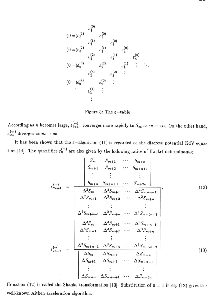
(46)Let us apply Thiele’s $\rho$-algorithm for two examples and compare its performance with the
$\rho$-algorithm (16). First we consider a sequence
$S_{m}= \sum_{k=1}^{m}\frac{1}{k^{3/2}}arrow 2.61237534868\cdots$, (47)
whose asymptotic behavior is given by
$s_{m} \sim S_{\infty}+\frac{c_{1}}{m^{1/2}}+\frac{c_{2}}{m^{3/2}}+\cdots$
.
(48)In eq. (48), $c_{i}(i=1,2, \ldots)$ are constants. We put $\sigma(x)=x^{1/2}$ in eq. (45) and compare the result
with the $\rho$-algorithm.
Next we consider the problem ofevaluating
$S_{\infty}= \int_{0}^{1}g(x)\mathrm{d}_{X}$ (49)
by the trapezoidal rule. Define $S_{m}$ by
If$g(x)$ is sufficientlysmooth, an asymptotic behavior of$S_{m}$ is given by
$S_{m}$ $=$ $S_{\infty}+ \frac{d_{1}}{m^{2}}+\frac{d_{2}}{m^{4}}+\frac{d_{3}}{m^{6}}+\cdots$ , (51)
$d_{1}= \frac{1}{12}\{g’(1)-g(\prime 0)\},$ $d_{2}=- \frac{1}{720}\{g^{\prime/}(\prime 1)-g(/\prime\prime 0)\},$$\cdots$
.
We put $g(x)=(0.05+x)^{-1/2}$in eq. (49) and apply Thiele’s $\rho$-algorithm with $\sigma(x)=x^{2}$
.
As one can seefrom Figures 4and 5, Thiele’s$\rho$-algorithm accelerates larger classesofsequences.
We should select $\sigma(x)$ in eq. (45) appropriately according to asymptotics of agiven sequence $S_{m}$
.
\S 6
The PGR algorithmsIn this section, we discuss the “PGR algorithms”. First of all, we consider the most general
form of the algorithm given by
$(x_{n+}-(m)X(m+1n-11))(x_{n}^{(1})_{-}x(m+m\rangle)=\mathcal{Z}(nnm)$. (52)
Papageorgiou et al. [4] applied the singularity confinement test to eq. (52). If we have $x_{n}$ $=$
$(m+1)$
$x_{n}^{(m)}+\delta$, then $x_{n+1}^{()}m$ diverges as $z_{n}^{(m)}/\delta$
.
At the next iteration, we find$x_{n+2}=x_{n}^{(}+(m)m+1)(1- \frac{z_{n+1}(m)}{z_{n}^{(m)}})\delta+O(\delta^{2}),$ $x_{n+2}^{\{)}m-1=x^{(}nm)+ \frac{z_{n+}^{(m_{1}}-1)}{z_{n}^{(m)}}\delta+o(\delta 2)$. (53)
The singularity confinement condition, i.e. $x_{n+}^{\langle 1)}m-3$ finite, is
$z_{n}^{(m)_{-z_{n}-z_{n+1}^{\mathrm{t}}+}}(m-1+1)m)z_{n+}^{\mathrm{t}^{m}-1)}2=0$
.
(54)The $\epsilon(z_{n}^{\mathrm{t}^{m}})=1),$ $\rho(z_{n}^{(m})=n)$, and Thiele’s $\rho(z_{n}^{(m)}=\sigma(m+n)-\sigma(m))$algorithms pass the above
condition (54). We call the most generalized class ofalgorithms (52), where $z_{n}^{(m)}$
satisfies eq. (54),
“the PGR algorithms”. It is interesting to remark that Brezinski and Redivo Zaglia [16] have
already proposed the algorithm (52) satisfying the singularity confinement condition (54), which
they termed “the homographic invariance”.
Two question arises; (1) what kind of integrable equations are the PGR algorithms associated
with ifthey are considered as difference equations? (2) howis the performance ofPGR algorithms
as convergence accelerators?
As one solution to the first question, we have recently found that it is related to the discrete
Painlev\’eequation of type I [17]. Weconsider a special case of the PGR algorithms,
which passes thesingurality confinement test. Through variable transformations,
$k=n-m,$ $l=m$, (56)
we have
$(X(k+1,l)-X(k-2, l+1))(X(k-1, l)-x(k, l))=k+C$
.
(57)Elimination ofthe dependence ofthe variable $l$ in eq. (57) gives thefollowing equation;
$X(k+1)-x(k-2)= \frac{-k-C}{X(k)-x(k-1)}$
.
(58)Through dependent variable transformation,
$Y(k)=X(k)-x(k-1)$
, (59)we have
$\mathrm{Y}(k+1)+\mathrm{Y}(k)+Y(k-1)=\frac{-k-C}{\mathrm{Y}(k)}$ (60)
from eq. (58). The equation (60) is nothing but the discretePainlev\’e equation oftypeI. It is noted,
however,the algorithm (55) does not accelerate convergence of sequences well.
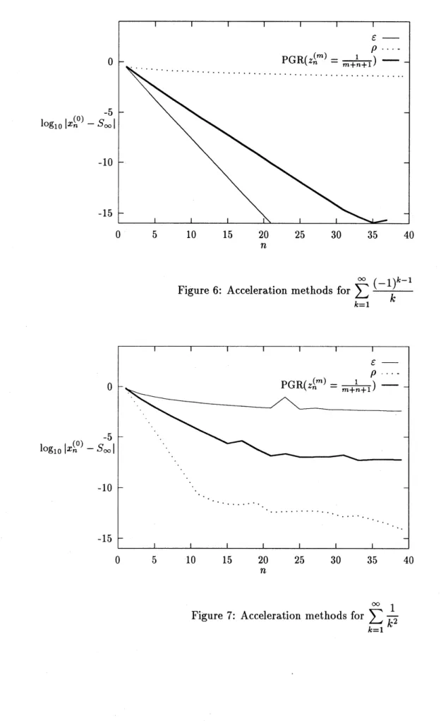
Let us go to the second question, i.e. acceleration performance of the PGR algorithms.
Intu-itively speaking, most ofthe PGR algorithms do not well accelerate convergence as far as we have
tested them. Among them, however, when we take
$z_{n}^{(m)}= \frac{1}{m+n+1}$, (61)
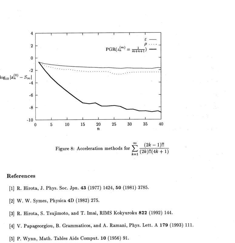
the algorithm accelerates both alternatively and rationally decayingsequences (See Figures 6–8).
\S 7
Concluding Remarks
We have shown there beingastrongtiebetweenconvergenceacceleration algorithms and discrete
soliton equations. It is a future problem to clarify how two different notions, acceleration and
integrability, are associated with each other. In other words, we should consider whether we can
construct new convergence acceleration algorithms from the other discrete soliton
equations2
andwhat kind of equations the other algorithms correspond to. The solution of these problems will
shed a new light on the study of discreteintegrable systems and numerical analysis.
It is a pleasure to thank Dr. Yasuhiro Ohta at Hiroshima University and Dr. Tetsu Yajima
at Tokyo University for many fruitful discussions on the subject. We would like to thank Prof.
Naoki Osada at Nagasaki Institute of Applied Science for valuable pieces of information on the
$\rho$-algorithm and the singularity confinement.
Appendix A Numerical Results
We here present numerical examples. In Figure 4 the $\rho$-algorithm and Thiele’s $\rho$-algorithms
are applied to the sequence $S_{m}= \sum_{k=1}^{m}\frac{1}{k^{3/2}}$
.
These two algorithms arealso applied to the numericalintegration for $\int_{0}^{1}\frac{1}{\sqrt{005+x}}\mathrm{d}X$ in Figure 5. We also employed $\epsilon$-algorithm,
$\rho$-algorithm, and
PGR algorithmwith $z_{n}^{(m)}= \frac{1}{m+n+1}$ toaccelerate the series,
$1- \frac{1}{2}+\cdots+\frac{(-1)^{m-1}}{m}+\cdotsarrow\log 2(=0.69314718\cdots)$,
(62)
$1+ \frac{1}{2^{2}}+\cdots+\frac{1}{m^{2}}+\cdotsarrow\frac{\pi^{2}}{6}(=1.6449336\cdots)$,
(63)
$\frac{1}{2\cdot 5}+\frac{1\cdot 3}{2\cdot 4\cdot 9}+\cdots+\frac{(2m-1)!!}{(2m)!!(4m+1)}+\cdotsarrow\int_{0}^{1}\frac{\mathrm{d}x}{\sqrt{1-x^{4}}}-1(=0.31102877\cdots)$, (64)
Figure 4: Acceleration methods for $\sum_{k=1}^{\infty}\frac{1}{k^{3/2}}$
$\cup$ $\perp\cup$ $10$ $\angle\cup$ $l\mathrm{O}$ $\delta\cup$
$n$
$i\mathrm{J}\theta$
Figure 6: Acceleration methods for $\sum_{k=1}^{\infty}\frac{(-1)^{k-1}}{k}$
$\cup$ $\perp\cup$ $1\theta$ $-l\cup$ Zb $\delta\cup$ $\mathrm{d}S$ $4\cup$
$n$
Figure 8: Acceleration methods for$\sum_{k=1}^{\infty}\frac{(2k-1)!!}{(2k)!!(4k+1)}$
References
[1] R. Hirota, J. Phys. Soc. Jpn. 43 (1977) 1424, 50 (1981) 3785.
[2] W. W. Symes, Physica4D (1982) 275.
[3] R. Hirota, S. Tsujimoto, and T. Imai, RIMS Kokyuroku 822 (1992) 144.
[4] V. Papageorgiou, B. Grammaticos, and A. Ramani, Phys. Lett. A 179 (1993) 111.
[5] P. Wynn, Math. Tables Aids Comput. 10 (1956) 91.
[6] F. L. Bauer, in: On Numerical Approximation, ed. R. E. Langer (University of Wisconsin
Press, Madison, 1959) p.361.
[7] T. N. Thiele, Interpolationsrechnung (Taubner, Leibzig, 1909).
[8] P. Wynn, Proc. Cambridge Philos. Soc. 52 (1956) 663.
[10] D. Levin, Int. J. Comput. Math. B3 (1973) 371.
[11] C. Brezinski, Lecture notes in mathematics, Vol. 584, Acc\’el\’eration de la convergence and
analyse num\’erique (Springer, Berlin, 1977).
[12] S. Maxon and J. Viecelli, Phys. Fluids. 17 (1974) 1614.
[13] D. Shanks, J. Math. Phys. 34 (1955) 1.
[14] H. W. Capel, F. W. Nijhoff, and V. G. Papageorgiou, Phys. Lett. A 155 (1991) 377.
[15] D. A. Smith and W. F. Ford, SIAM J. Numer. Anal. 16 (1979) 223.
[16] C. Brezinski and M. Redivo Zaglia, Extrapolation Methods. Theory and Practice
(North-Holland, Amsterdam, 1991).