On the Markoff-Painleve Transcendent (Integrated Research on Complex Dynamics and its Related Fields)

(1)

Katsunori Iwasaki

(

岩崎克則

)

Faculty

of

Mathematics,

Kyushu University,

Fukuoka

819-0395

Japan*

March

29,

2010

Abstract

All positive integral solutions to Markoff’s equation are in one-to-one

correspon-dence with all analyticcontinuations ofatranscendentalsolutiongermtoaspecialsixth

Painlev\’e equation via the Riemann-Hilbert correspondence. We explicitly determine

the parameter value and the initial condition for the Markoff-Painlev\’e transcendent.

1 Markoff’s Diophantine Equation

In 1879 and 1880 A.A. Markoff [9, 10] discussed a Diophantine equation of the form

$m_{1}^{2}+m_{2}^{2}+m_{3}^{2}=3m_{1}m_{2}m_{3}$ $(m_{1}, m_{2}, m_{3})\in \mathbb{N}^{3}$, (1)

in thestudy ofbadly approximable irrational numbers and indefinite binary quadratic forms.

We present

some

known facts about Markoff’s equation (1) (see e.g. [1]). It has the

trivial solution (1, 1, 1). It also has another simple solution (1, 1,2). These two solutions

are

referred to

as

the exceptionalsolutions. Any other solution is called a regularsolution. Any

regular solution has mutually distinct components. There are infinitely many solutions and

there is a simple algorithm which produces all of them. It is based on a large symmetry

$G=\langle\sigma_{1},$ $\sigma_{2},$$\sigma_{3}\}\cong \mathbb{Z}_{2}*\mathbb{Z}_{2}*\mathbb{Z}_{2}$ leaving equation (1) invariant, where $\sigma_{1}$ is the involution $\sigma_{1}$ : $(m_{1}, m_{2}, m_{3})\mapsto(3m_{2}m_{3}-m_{1}, m_{2}, m_{3})$, (2)

with $\sigma_{2}$ and $\sigma_{3}$ being defined in similar manners. Two solutions are said to be $n$eighbors if

they share two components. Any regular solution $(m_{1}, m_{2}, m_{3})$ has exactly three neighbors

$\sigma_{i}(m_{1}, m_{2}, m_{3}),$ $i=1,2,3$, one smaller and two larger, where the ordering is defined by

$(m_{1}, m_{2}, m_{3})\prec(m_{1}, m_{2}’, m_{3})$ if $\max\{m_{1}, m_{2}, m_{3}\}<\max\{m_{1}, m_{2}, m_{3}’\}$.

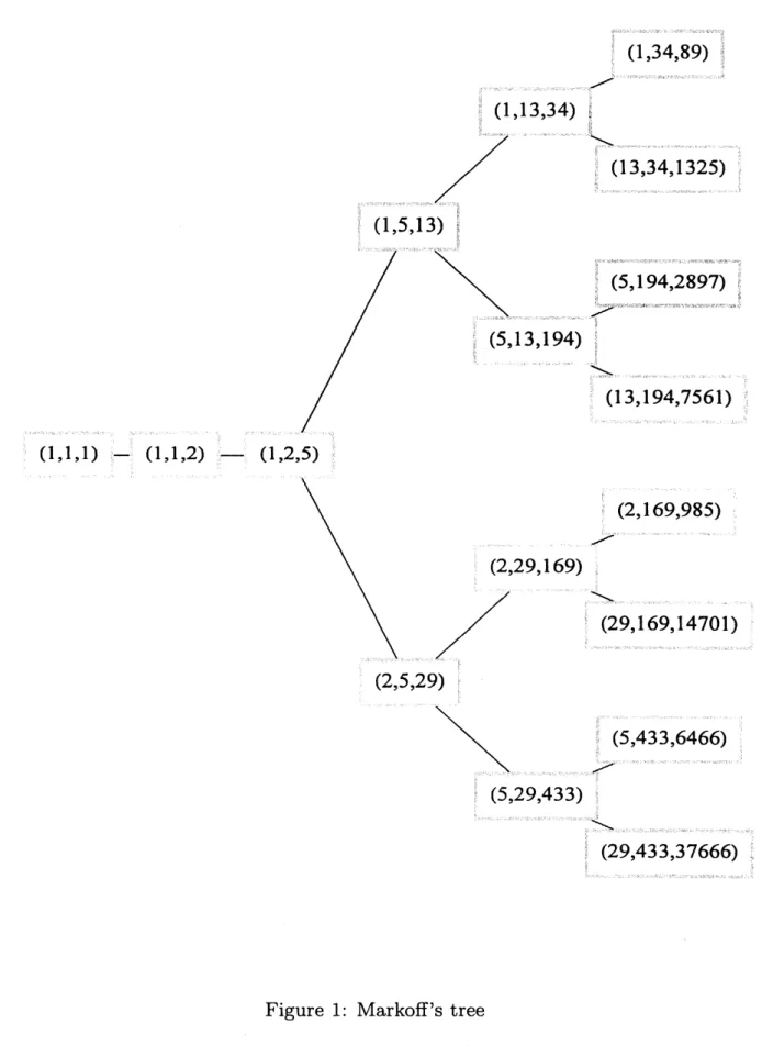
Starting with the trivial solution (1, 1, 1), apply $\sigma_{1},$ $\sigma_{2},$ $\sigma_{3}$ recursively in all possible ways

to produce infinitely many solutions. This process can be incorporated into a tree in Figure

1, which is known

as

Markoff’s tree. Any solution

occurs

exactly once in the tree and the

G-orbit through the trivial solution (1, 1, 1) constitutes all the solutions to equation (1).

The aim of this note is to throw a bridge between the Markoff orbit and a very special

solution to the sixth Painlev\’e equation via the Riemann-Hilbert correspondence.

(2)

$”$ $\nu$ $\sim\phi$

(1,1,1) – (1,1,2) –

$\nu*-a-,$

$\alpha\sigma_{\ovalbox{\tt\small REJECT}^{\nwarrow_{m---\sim x\cross*-*_{\ovalbox{\tt\small REJECT}}}} ,8_{*-RM’ 8\ovalbox{\tt\small REJECT} M\alpha x\infty\infty R\lambda^{*}}^{8}(29,433,37666)_{*}^{2}}$

(3)

Figure 2: Monodromy map $\gamma_{*}$ : $\mathcal{M}_{z}(\kappa)O$ along

a

loop $\gamma\in\pi_{1}(Z, z)$

.

2 The

Sixth

Painlev\’e

_Equation

The sixth Painlev\’e equation $P_{VI}(\kappa)$ is a Hamiltonian system

$\frac{dq}{dz}=\frac{\partial H(\kappa)}{\partial p}$, $\frac{dp}{dz}=-\frac{\partial H(\kappa)}{\partial q}$, (3)

with a complex time variable $z\in Z$ $:=\mathbb{P}^{1}-\{0,1, \infty\}$ and unknown functions $q=q(z)$ and

$p=p(z)$, depending on complex parameters $\kappa$ in the four-dimensional affine space

$\mathcal{K}:=\{\kappa=(\kappa_{0}, \kappa_{1}, \kappa_{2}, \kappa_{3}, \kappa_{4})\in \mathbb{C}_{\kappa}^{5}:2\kappa_{0}+\kappa_{1}+\kappa_{2}+\kappa_{3}+\kappa_{4}=1\}$,

where the Hamiltonian $H(\kappa)=H(q,p, z;\kappa)$ is given by

$z(z-1)H(\kappa)=(q_{0}q_{z}q_{1})p^{2}-\{\kappa_{1}q_{1}q_{z}+(\kappa_{2}-1)q_{0}q_{1}+\kappa_{3}q_{0}q_{z}\}p+\kappa_{0}(\kappa_{0}+\kappa_{4})q_{z}$ ,

with $q_{\nu}$ $:=q-\nu$ for $\nu\in\{0, z, 1\}$. Any meromorphic solution germ at any point $z\in Z$ admits

a global meromorphic continuation along any path in $Z$ emanating from $z$. This property is

known as the Painleve propertyfor the sixth Painlev\’e equation [2].

Let $\mathcal{M}_{z}(\kappa)$ be the set of all meromorphic solution germs to equation (3) at a base point

$z\in Z$. It is realized as the moduli space of (certain) stable parabolic connections, thereby

provided with the structure of a smooth quasi-projective rational complex surface, where

a

stable parabolic connection is a rank-two vector bundle

over

$\mathbb{P}^{1}$ together with

a Fuchsian

connection having four regular singular points and a parabolic structure that satisfies a sort

of stability condition in geometric invariant theory [2, 3, 4].

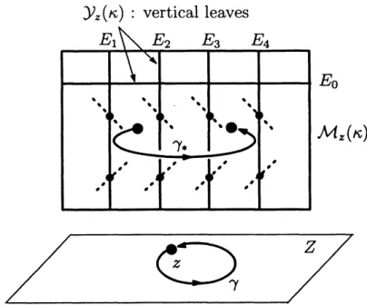
By the Painlev\’e property, any solution germ $Q\in \mathcal{M}_{z}(\kappa)$ continues analytically along

any loop $\gamma\in\pi_{1}(Z, z)$. Let $\gamma_{*}Q$ be the result of the analytic continuation. Then the map

(4)

Figure 3: Dynkin diagram of type $D_{4}^{(1)}$

is a holomorphic automorphism of $\mathcal{M}_{z}(\kappa)$ (see Figure 2), which is called the monodromy

map along the loop $\gamma$. It represents the multi-valuedness along $\gamma$ of the solution germs.

3 Affine

Weyl

Groups

and

Stratification

The parameter space $\mathcal{K}$ of Painlev\’e VI admits

some

affine

Weyl group actions, in terms of

which $\mathcal{K}$ carries a

natural stratification. We shall now describe these structures [6, 7, 8].

The standard complex Euclidean inner product

on

$\mathbb{C}_{\kappa}^{4}$ induces an inner product

on

$\mathcal{K}$

through the forgetful isomorphism $\mathcal{K}arrow \mathbb{C}_{\kappa}^{4},$ $(\kappa_{0}, \kappa_{1}, \kappa_{2}, \kappa_{3}, \kappa_{4})\mapsto(\kappa_{1}, \kappa_{2}, \kappa_{3}, \kappa_{4})$

.

For each

$i\in\{0,1,2,3,4\}$ let $w_{i}$ : $\mathcal{K}O$ be the orthogonal reflection in the affine hyperplane _{$H_{i};=$}

$\{\kappa\in \mathcal{K} : \kappa_{i}=0\}$. These five reflections generate an affine Weyl group of type $D_{4}^{(1)}$, $W(D_{4}^{(1)})=\langle w_{0},$

$w_{1},$ $w_{2},$ $w_{3},$ $w_{4}\rangle\cap \mathcal{K}$.

Denote the nodes of the Dynkin diagram $D_{4}^{(1)}$ by _{$\{0,1,2,3,4\}$}

as

in Figure 3. The

automor-phism group of the Dynkin diagram $D_{4}^{(1)}$ is the symmetric group $S_{4}$ of degree 4 permuting

{1,

2, 3,

_4}

while fixing the central node $0$. The semi-direct product

$W(F_{4}^{(1)}):=W(D_{4}^{(1)})\rangle\triangleleft S_{4}\cap \mathcal{K}$

is an affine Weyl group oftype $F_{4}^{(1)}$, which is the full symmetry group of Painlev\’e VI.

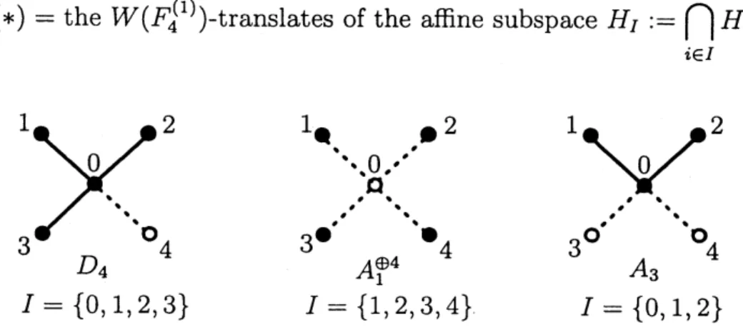
Given a proper subdiagram $*$ of the Dynkin diagram $D_{4}^{(1)}$, let _$I$ be a proper subset of

$\{0,1,2,3,4\}\}$ representing $*$

.

The closed stratum associated with $*$ is then defined by $\overline{\mathcal{K}}(*)=$ the $W(F_{4}^{(1)})$-translates of the affine subspace _{$H_{I}$}

$:= \bigcap_{i\in I}H_{i}$, $1_{\bullet}$

.

$\bullet^{2}$ $0,$’ $\backslash Q$

.

.’

..

$3^{\bullet’}$ $\bullet_{4}$ $A_{1}^{\oplus 4}$

$I=\{0,1,2,3\}$ $I=\{1,2,3,4\}$ $I=\{0,1,2\}$

(5)

$\emptysetarrow A_{1}A_{2}\downarrowarrowarrow A_{1}^{\oplus 2}A_{3}\downarrowarrowarrow A_{1}^{\oplus 3}D_{4}\downarrowarrow A_{1}^{\oplus 4}$

Figure 5: Adjacency relations among the strata

4 Riemann-Hilbert

Correspondence

The study of Painlev\’e equation is developed not directly

on

the moduli space $\mathcal{M}_{z}(\kappa)$, but

by passing to

a

character variety $S(\theta)$ via the Riemann-Hilbert correspondence [2, 3, 4, 8],

RH$z,\kappa$ :

$\mathcal{M}_{z}(\kappa)arrow S(\theta)$, $Q\mapsto\rho$, with $\theta=$ rh$(\kappa)$

.

(4)

Here the character varieties for Painlev\’e VI

can

be realized

as a

four-parameter family of

complex affine cubic surfaces $S(\theta)=\{x=(x_{1}, x_{2}, x_{3})\in \mathbb{C}^{3} : f(x, \theta)=0\}$ with

$f(x, \theta):=x_{1}x_{2}x_{3}+x_{1}^{2}+x_{2}^{2}+x_{3}^{2}-\theta_{1}x_{1}-\theta_{2}x_{2}-\theta_{3}x_{3}+\theta_{4}$, (5)

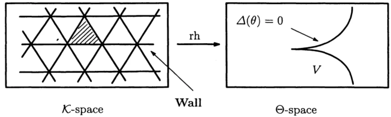
parametrized by $\theta=(\theta_{1}, \theta_{2}, \theta_{3}, \theta_{4})\in\Theta$ $:=\mathbb{C}^{4}$ and rh : $\mathcal{K}arrow\Theta$ is a holomorphic map which is

a branched $W(D_{4}^{(1)})$-covering ramifying along Wall (the union ofall reflection hyperplanes)

and mapping it onto the discriminant locus $V$ $:=\{\theta\in\Theta : \Delta(\theta)=0\}$ of the cubic surfaces

(see Figure 6). A fundamental fact for the map (4) is the following.

Theorem 1 ([2, 3, 4])

_If

$\kappa\in \mathcal{K}(*)$ then the character variety $S(\theta)$ with $\theta=$ rh$(\kappa)$ has

simple singularities

_of

Dynkin $type*and$ the Riemann-Hilbert correspondence (4) is a proper

surjective holomorphic map that gives an analytic minimal resolution

_of

$S(\theta)$.

Wall

$\mathcal{K}$-space $\Theta$-space

(6)

Figure 7: Three basic loops in $\pi_{1}(Z, z)$, where _{$z_{1}=0,$ $z_{2}=1$} and _{$z_{3}=\infty$}

.

Take an algebraicminimal desingularization$\varphi$ : $\tilde{S}(\theta)arrow S(\theta)$. Then the Riemann-Hilbert

correspondence (4) uniquely lifts to a biholomorphism RH$z,\kappa$ :

$\mathcal{M}_{z}(\kappa)arrow\tilde{S}(\theta)$ such that $\mathcal{M}_{z}(\kappa)arrow^{\overline RH_{z,\kappa},}\tilde{S}(\theta)$

$\Vert$ $\downarrow\varphi$

$\mathcal{M}_{z}^{-}(\kappa)\underline{RH_{z,\kappaarrow}}S(\theta)$

is commutative. Via the lifted Riemann-Hilbert correspondence $\overline{RH}_{z,\kappa}$, the monodromy map

$\gamma_{*}:\mathcal{M}_{z}(\kappa)O$ is strictly conjugate to an automorphism $\sigma$ : $\tilde{S}(\theta)O$ in a way shown below.

The cubic surface $S(\theta)$ admits three involutive automorphisms

$\sigma_{i},$ $i=1,2,3$, where

$\sigma_{1}:(x_{1}, x_{2}, x_{3})\mapsto(\theta_{1}-x_{1}-x_{2}x_{3}, x_{2}, x_{3})$, (6)

with $\sigma_{2}$ and $\sigma_{3}$ beingdefined_{$in_{\sim}similar$}

manners.

They lift in aunique way toautomorphisms

of the desingularized surface $S(\theta)$, which will be denoted by the

same

symbols

$\sigma_{i}$. On the

other hand the fundamental group $\pi_{1}(Z, z)$ is represented as

$\pi_{1}(Z, z)=\langle\gamma_{1},$$\gamma_{2},$$\gamma_{3}|\gamma_{1}\gamma_{2}\gamma_{3}=1\rangle$,

where $\gamma_{i},$ $i=1,2,3$ , are the basic loops

as

in Figure 7. For each $i=1,2,3$ , the monodromy

map along the loop $\gamma_{i}$ is conjugate to the automorphism

$\sigma_{i+1}\sigma_{i}$ of $\tilde{S}(\theta)$, where the index $i$

should be considered modulo 3, via the lifted Riemann-Hilbert correspondence.

Let $G$ be the group generated by the three involutions

$\sigma_{1},$ $\sigma_{2},$ $\sigma_{3}$. It is a universal Coxeter group of rank three, having the only relations $\sigma_{1}^{2}=\sigma_{2}^{2}=\sigma_{3}^{2}=1$

.

Let $G(2)$ be the

index-two subgroup of all even words in $G$. The last paragraph says that the monodromy

action $\pi_{1}(Z, z)\cap \mathcal{M}_{z}(\kappa)$ is faithfully represented by the group action $G(2)\cap\tilde{S}(\theta)$

.

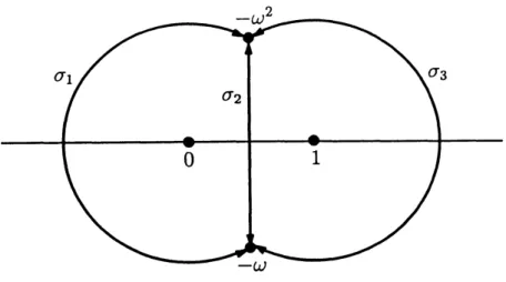
Thus

the full group action $Gc\sim\tilde{S}(\theta)$ may be thought of as faithfully representing the

“half-monodromy” action. The corresponding (half-loops” are depicted in Figure 8, where the

half-loop corresponding to $\sigma_{i}$ is denoted by the

same

symbol $\sigma_{i}$ and $\omega$ $:=\exp(2\pi i/3)$. The

(7)

Figure 8: Three half-loops: the point at infinity is invisible

5 The

Markoff-Painlev\’e

Thranscendent

If we put $(x_{1}, x_{2}, x_{3})=(-3m_{1}, -3m_{2}, -3m_{3})$, then formula (5) implies that the Markoff

cubic (1) is just the cubic surface $S(\theta)$ with parameters $(\theta_{1}, \theta_{2}, \theta_{3}, \theta_{4})=(0,0,0,0)$ and the

involution (2) agrees with the involution (6). Moreover we observe that

$( \kappa_{0}, \kappa_{1}, \kappa_{2}, \kappa_{3}, \kappa_{4})=(-\frac{1}{4},$ $\frac{1}{2},$ $\frac{1}{2},$ _{$\frac{1}{2},0)\in \mathcal{K}(A_{1})$} (7)

lies over $\theta=(0,0,0,0)$ relative to the small Riemann-Hilbert correspondence rh: $\mathcal{K}arrow\Theta$

.

The main theorem of this note is now stated

as

follows.

Theorem 2 Via the Riemann-Hilbert correspondence (4), the

_Markoff

orbit in Section 1

corresponds to all the analytic continuations

_of

the solution germ to equation (3) with

pa-rameters (7) that

_satisfies

the initial condition

$(q,p)=( \frac{i\omega^{2}}{\sqrt{3}},0)$ at _$z=-\omega$.

The proofof this theorem will be given elsewhere.

References

[1] E. Bombieri, Continued fractions and the Markoff tree, Expo. Math. 25 (2007), no. 3,

187-213.

[2] M. Inaba, K. Iwasaki and M.-H. Saito, Dynamics of the sixth Painle$\backslash ’\acute{e}$ equation,

Th\’eories asymptotiques et \’equations de Painlev\’e, S\’eminaires et Congr\‘es 14, (2006),

103-167.

[3] M. Inaba, K. Iwasaki and M.-H. Saito, Moduli ofstableparabolicconnections,

Riemann-Hilbert correspondence and geometryof Painleveeq uation oftype VI. PartI, Publ. Res.

(8)

[4] M. Inaba, K. Iwasaki and M.-H. Saito, Moduli ofstable parabolicconnections,

Riemann-Hilbert correspondence and geometry ofPainlev\’e equation of type VI. Part II, Adv.

Stud. Pure Math., 45 (2006), 387-432.

[5] K. Iwasaki, An area-preserving action of the modular group on cubic surfaces and th$e$

Painle

ve

VI equation, Comm. Math. Phys. 242 (1-2) (2003), 185-219.

[6] K. Iwasaki, Finite branch solutions to Painlev\’e VI

aro

und

a

fixed singular point, Adv.

Math., 217 (2008),

no.

5, 1889-1934.

[7] K. Iwasaki and T. Uehara, An ergodic study of Painleve VI, Math. Ann., 338 (2007),

no. 2, 295-345.

[8] K. Iwasaki and T. Uehara, Singular cubic surfaces and th

e

dynamics ofPainlev\’e VI,

e-Print arXiv:

0909.5269

[math.AG] 29 Sep 2009, 34 pages.

[9] A.V. Markoff, Sur les forms quadratiques binaires ind\’efinies, Math. Ann. 15 (1879),

381-409.

[10] A.V. Markoff, Sur les forms quadratiques binaires ind\’efinies, Math. Ann. 17 (1880),