Symbolic-Numeric Optimization for Estimation of Parameters in a Biological Kinetic Model(Computer Algebra : Design of Algorithms, Implementations and Applications)

Symbolic-Numeric Optimization

for Estimation

of

Parameters

in

a

Biological Kinetic Model

折居茂夫

堀本勝久

SHIGEO ORII KATSUHISA HORIMOTO

富士通株式会社

産業技術総合研究所・生命情報科学研究センター

FUJITSU LTD * _{COMPUTATIONALBIOLOGY RESEARCE CENTER, AIST} \dagger

穴井宏和

HIROKAZU ANAI

(

株

)

富士通研究所

/(

独

)

科学技術振興機構

FUJITSU

LABORATORIES LTD $/\mathrm{C}\mathrm{R}\mathrm{E}\mathrm{S}\mathrm{T}$

,

JST $\mathrm{t}$

Abstract

We have beenstudying asymbolic-numeric optimization forestimation of $\mathrm{p}\mathrm{a}\mathrm{r}\mathrm{a}\mathrm{m}\mathrm{e}\mathrm{t}\mathrm{e}\infty$ inbiological

kinetic modelsbyquantifierelimination $(\mathrm{Q}\mathrm{E})$, incombination with numerical simulation methods. The

optimization methodwasappliedtoamodel for the inhibition kineticsofHIVproteinasewithten param-etersand nine variables. Weapply this optimization procedureto three sets of observed dataandobtain kineticparametersby usingonlyonepointof each set of the data.

1

Introduction

Many methods for local and globaloptimization havebeen developedto model and simulate the global

network of biological molecules inacell$[1, 2]$, andsomesimulators basedon variousoptimization methods

have also beendesigned (e.g. [3]). Intheoptimization methods,the estimation of kineticparametersplays

a

keyroleinthedevelopment of kinetic models, which, in turn,promotesfunctionalunderstanding atthe

system level, for example, in several biological pathways $[4, 5]$

.

Ananswer totheestimation of kinetic

parametersisoursymbolic-numeric optimization which combines symbolic QE with numerical simulation

$[6, 7]$

.

In this paper,firstly,weshow

our

procedureoftheoptimizationfor the inhibition kinetics of HIV

proteinase [8],whichincludes

an

enhancedprocedureofthe offsetcomputation. Secondly,

we

showthat

the kinetic parameters forthreesets of obeerved data

can

be estimatedbyusingonly

one

pointof each

set of the data.

$\mathrm{r}_{\mathrm{o}\mathrm{r}\mathrm{i}\mathrm{i}0*\mathrm{t}\mathrm{r}\mathrm{a}\mathrm{d}.\mathrm{r}\mathrm{g}.\mathrm{f}\mathrm{i}_{\mathrm{t}\mathrm{i}^{\mathrm{i}\mathrm{t}\epsilon \mathrm{u}.\infty \mathrm{m}}}}$

$\uparrow \mathrm{h}\mathrm{o}\mathrm{r}\mathrm{l}\mathrm{m}\mathrm{o}\mathrm{t}\mathrm{o}\mathrm{O}\mathrm{c}\mathrm{b}\mathrm{r}\mathrm{c}.\mathrm{j}\mathrm{p}$

2

MATERIALS AND METHODS

2.1

Mathematical

Framework

Problem: In thispaper,

we

considerthe$\mathrm{f}\mathrm{o}\mathrm{U}\mathrm{o}\mathrm{w}\mathrm{i}\mathrm{n}\mathrm{g}$ fitting problem: thebiological kinetic model analyzed

here isoftheform:

$\dot{x}_{1}=v:(X,K)$ (1)

where$X=\{x_{1}, \cdots,x_{n_{\mathrm{s}}}\}$isaset ofvariables,and$K=\{k_{1}, \cdots, k_{n_{\dot{f}}}\}$is

a

set of parameters. The problem

istofit the parameters$K$of the model totheobserved data$\tilde{X}=\{\tilde{x}_{l}^{\ell}\}$ for,$i=1,$

$\cdots,n_{x},$$t=0,1,$$\cdots,n_{\overline{x}_{\mathrm{t}}}$

underthefollowing additionalconditions:

(i)Conservation laws: $h_{:}(X)=0$

(ii)Variableranges: $X:\in D_{i}$, where$D_{:}=[a, b],$$a,$$b\in \mathbb{R}\cup\{\infty\}$

.

Basic librmula Herewe set up theleading formula ofthispaper. As mentioned above, wehave the

followingconstraints$\Psi$with

error

variables ei fromkineticmodels: $\Psi\equiv\bigwedge_{*}\psi_{:}$,where$\psi_{i}=\dot{x}:-v_{1}(X,K)+$

$e_{j}=0$

.

Forthe

error

variables weintroduce

a

new

variable, $e_{[][]},ax$, which meansthemagnitude ofthe

error

variables: $|e.|\leq e_{\max}$

.

Moreover, for the variableswhoseobserved data is given,

we

considerthe

following objectiveconditions: $X_{l}^{(t)}-\overline{X}_{l}^{(t)}=0$, toachieve fitting. Then the

.

basicformula

’

isgiven

as

$F(\dot{X}, X, K, e_{\max}, e:)\equiv$($\Psi$A$h_{:}(X)=0$A$X:\in D_{1}\wedge|e_{i}|\leq e_{\max}$A$X_{l}^{(t)}-\overline{X}_{l}^{\langle t\rangle}=0$). (2)

We apply

our

symbolic-numeric approach to formulas derivedby slightly modifying the basic formula

accordingtovariouspurposes.

2.2

Optimization

Procedure

We explainthe concreteprocedureofsymbolic-numeric optimization,whichconsists of sixparts as

illustratedin Figure1.

(1)Numerical simulation Firstweprepare simulationdatafor$\dot{x}$

:and$X:$,for whichwelackobserved

data, byperforminganumerical simulation of the kinetic models. 1. Set initial conditions $\tilde{X}^{(0\rangle}$

and starting values for unknown parameters $\overline{K}^{\langle 0)}$

as

follows: $\overline{X}^{(0)}\equiv$

$\{\tilde{x}^{(0)}|i=1, \cdots, n_{x}\}$ and $\overline{K}^{(0)}=K_{1}^{(0)}\cup K_{2}^{(0)}$, where $\overline{K}_{1}^{(0)}\equiv\{k_{1}^{(0)}, \cdots, k_{j}^{(0)}\}$ are starting values, and

$\tilde{K}_{2}^{(0)}\equiv\{k_{j+1}^{(0)}, \cdots, k_{n_{j}}^{(0)}\}$

are

givenfxed pwameters.

2. By numerical simulation of the kinetic model (1), we obtain

a

time series for $x$: and $\dot{x}_{1}:X_{i}^{(t)}=$

$\{x_{i}^{(t)}|i=1, \cdots n_{1},t)=0,1, \cdots,n_{t}\}$and$\dot{X}_{1}-(.\ell)=\{\overline{\dot{x}}_{i}^{(t)}|i=1, \cdots,n:, t=0,1, \cdots,n_{t}\}$

.

(2) liormulation Afterchoosingsome variablesfrom$X$,

we

callthem

$\ell$

focusing$\mathrm{v}\mathrm{a}\mathrm{r}\mathrm{i}\mathrm{a}\mathrm{b}\mathrm{l}\infty’,$ $\mathrm{Y}$, and

substitute$\mathrm{o}\mathrm{b}\mathrm{s}\mathrm{e}\mathrm{r}\mathrm{v}\mathrm{e}\mathrm{d}/\mathrm{s}i\mathrm{m}\mathrm{u}\mathrm{l}\mathrm{a}\mathrm{t}\mathrm{e}\mathrm{d}$ data into theremainingvariables:

1. Choose

a

subset$\mathrm{Y}$ of_$X$:$Y\subseteq X$

.

2.

Substitute$\dot{X}$,

$X\backslash \mathrm{Y}$, in $F$bythe values of

$\tilde{\dot{X}},\overline{X}$ at

a

time point $t:\dot{X}_{i}arrow\overline{\dot{X}}_{1}^{(\ell)}.,\dot{X}:arrow\dot{X}_{i}^{(l)}$

,

where

$x:\in\tilde{\dot{X}},X\backslash Y$

.

Then

we

denote the

new

formula

as

$F’(\mathrm{Y},K_{1},e_{\max’:}e)$

.

Wenote by$\mathrm{p}\mathrm{e}\mathrm{r}\mathrm{f}\mathrm{o}\mathrm{r}\mathrm{n}\dot{\mathrm{u}}\mathrm{n}\mathrm{g}$

a

QE

Figure1: Flowchart ofsymbolic-numeric optimization. Thevariablesandvsluesareenclosedby the boxes, and the proceduresarenumbered corresponding to the description in the text.

(3) Computation ofoffset by QE Observeddataoften contain anoffset. Therefore,wemust first

determine theoffsetvalue. Hereweconsider the

case

that the offsetappearslinearly. For the sake of

sim-plicity,we

assume

thatonly$\overline{x}_{1}$hasanoffset. Let

$F_{off\epsilon\epsilon t}’$bethe formulaobtained by putting$\overline{x}_{1}’$

-offset

into$\tilde{x}_{1}^{(\iota)}$ of_$F$‘, where

offset

is avariable for offset. By performing QE for $\exists X\exists K_{1}\exists e_{\max}\exists e_{j}(F_{\circ ff\epsilon\epsilon t}’)$,

we

obtainthe quantifier-hee formula $\pi(offset)$, which stands for the feasible

ranges

of

offset.

_Then

wesubstitute theminimum value of the offiet for the variable offset in $F’$

,

and wedenote it again by

$F’(\mathrm{Y},K_{1},e_{maae:},e)$

.

(4)Estimation of

emax

by QE First,

we

use

QE to find themagnitudeof

emax

assmallaspossible.

Bycomputing QEfor$F’(\mathrm{Y}, K_{1}, e:)$, we obtain aquantifier-free formula_$\pi(emax)$ describing thefeasible

ranges

of

emax.

Next,

we

put the minimum valueof$e_{\max}$ into $e_{\max}$ in $F’$, and denote the resulting

formula

as

$F”(\mathrm{Y},K_{1},e_{i})$

.

And Estimation of $K_{1}$ by QE We obtain a quantifier-free formula $\tau(K_{1})$ describing the feasible

ranges of$K_{1}$ by computing QEfor$\mathrm{Y}\exists e:(F’’)$,Actually, thefeasiblerangesof$K_{1}$

are

usuallysufflciently

narrow

intervals (e.g., about $10^{-6}$) to choose

an

appropriate specific_valueof_{$K_{1}$}

.

(5) Computationof

sum

of squares$(SSq)$ by numerical_{simulation We estimate the}

goodness-of-fitfor the obtainedparameter$\mathrm{v}\mathrm{a}\mathrm{l}\mathrm{u}\mathrm{a}\mathrm{e}K_{1}\mathrm{h}\mathrm{o}\mathrm{m}$thefeasibleranges$\mathrm{o}\mathrm{f}K_{1}$ in terms of$SSq$

.

1. Setinitialconditions$\overline{X}^{(0)}$ and$K_{1}$

.

2. Perform numerical simulationofkinetic model(1).

(6)$\mathrm{T}\mathrm{e}\mathrm{r}\mathrm{m}\mathrm{i}\mathrm{n}\mathrm{a}\mathrm{t}\mathrm{i}\mathrm{o}\mathrm{n}$ If$SSq$ issmallerthanaspecificlevel$\theta$, output $K$. Otherwise, set newinitial values

andgo to (1).

2.3

Biological

Model

We analyzed

a

model for the inhibition kinetics of

HIV proteinase [8],

as

shown in Figure 2. The

pro-teinase

monomer

$(M)$ is inactive, but the enzyme $(E\rangle$

$hf+Mr^{-}arrow$ $E$ $k_{11}(arrow)$

.

$k_{1arrow},(arrow)$

$S+E$ $\Leftrightarrow$

ES $k_{21},$$k_{2}\underline,$

is active in the dimeric form. The dimer catalyzes

ES $arrow$ $E+P$ $k_{3}$

the conversion ofthe substrate $(S)$ to theproduct $(P)$

.

$E+P$ $\underline{arrow}$ $EP$ $k_{41},$ $k_{42}$

The inhibitor (I) is competitive for the substrate and $E+I$ $-arrow$ _$EI$ $k_{51},$ $k_{S2}$

the product, and the inhibitor-binding enzyme is irre $EI$ $arrow$ _$EJ$ $k_{6}$

versibly deactivated $(EJ)$

.

In the model, there

are

ten

parameters and nine variables. According to the

previ-Figure 2: Kinetic model for the inhibitor of HIV

ous

studies $[8, 9]$,five parameters $(k_{11},k_{12}, k_{21}, k_{41}, k_{51})$

proteinase. The start values for ten parameters

are

given, and the remaining five unknown parameters and the initial values for nine variables[9] areas

$(k_{22}, k_{3},k_{42}, k_{52}, k_{6})$, two initialvalues $(E_{|n|\iota}, S_{1nu})$ and follows:

$k_{11}=0.1,k12=10^{-4},k_{21}=1\alpha 1,k\mathrm{a}2=$

$300,k_{\theta}=10,k_{41}=1\infty,k_{42}=500,$$k_{51}=10$ theoffietof the fluorimeterareestimated by thepresent , $k_{62}=0.1,andk_{6}=0.1;\overline{x}_{1}=0,\overline{x}\mathrm{a}=0.004,\overline{x}_{3}=$

method. The experimental data of the product $[P]$, 25.0,$\tilde{x}_{4}=0,\tilde{x}\mathrm{s}=0,\tilde{x}_{l}=0,\overline{x}_{7}=$ 0.003,$\tilde{x}_{8}=$

$0,and\overline{x}_{9}=0$

.

which are composedof 300 data points measured from

$0$ to 3600 seconds,

were

dowtoaded from

a

web site

(http:$//\mathrm{w}\mathrm{w}\mathrm{w}$

.

gepasi.$\mathrm{o}\mathrm{r}\mathrm{g}/\mathrm{t}\mathrm{u}\mathrm{t}\mathrm{o}\mathrm{r}\mathrm{i}\mathrm{a}\mathrm{l}\epsilon/\mathrm{o}\mathrm{p}\mathrm{t}/\mathrm{h}\mathrm{i}\mathrm{v}\mathrm{f}\mathrm{i}\mathrm{t}$

.

html).

3 RESULTS

First,we willdescribe thepracticalprocedurefor parameter optimization in the kinetic model forHIV

proteinaee, and then

we

will evaluate theoptimized parameters by using only

one

pointof the observed

data.

3.1

Procedure for

Optimizing

Parameters in HIV inhibition Model

To perform the numerical simulation (in (1) of 2.2),$K_{1}$ and $K_{2}$,

are

defined

as

the flve unknown

parameters andthe fivegiven parameters,andthe nine variablesareallocated to$[P],$ $[E],$ $[S],$ [ES], $[M]$,

$[EP],$ $[I],$ $[EI]$, and $[EJ]$

.

Thenweset the start value$\tilde{K}^{(0)}$ andtheinitial value$\tilde{X}^{(0)}$

.

The start values

for tenparametersandtheinitialvalues forninevariables

are

cited from the previousstudy [9] (seethe

legendinFigure2). Ako, the two initialvalues,Einit andSinit,

are

changed withinalimited range with

reference to thepreviousstudies $[8, 9]$: 31discrete values for$([E]=0.00350,0.00355, \cdots, 0.00500)$ and13

valuesfor $([S]=\mathit{2}3.0,\mathit{2}3.5, \cdots, 29.0)$

.

Thefocusingvariables$\mathrm{Y}$ (in (2)of2.2)aresimplyobtainedby the

symbolic computation with QEbom therelationship between$X\mathrm{a}\mathrm{n}\mathrm{d}K_{1}$inthe model. In theinequality

$v_{i}(X,K)\Delta t+x_{j}^{t}\geq 0$, the ehmination of$\Delta t$ by QE outputs five inequalities including five parameters:

$100*[E]*[I]-k5\mathit{2}*[EI]-k6*[EI]>0,100*[E]*[I]-k5\mathit{2}*[EI]>0,100*[E]*[P]-k42*[EP]-k3*[ES]<$

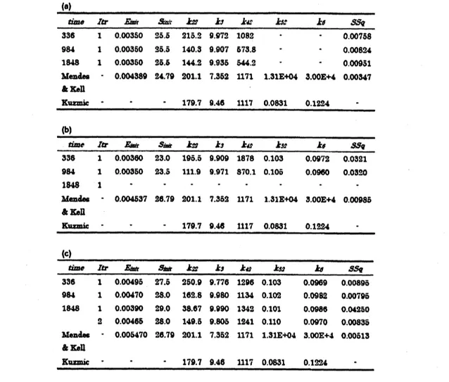
Table 1: Goodness of fit with optimized parameters by symbolic-numeric method. (a) is inthecase of

$\mathrm{I}=0$, which

means

noinhibition. (b) is inthe

case

of_{$\mathrm{I}=0.0015$}

.

$(\mathrm{c})$is inthe caseof$\mathrm{I}=0.003$

.

_$Itr$ is the

iterations number of thesymbolic-numeric optimization.

$.=\mathit{3}3610_{-\infty \mathrm{s}50}[\epsilon)\varpi eI\mathrm{f}\mathrm{f}\ \mathrm{r}\cdot \mathrm{a}\mathrm{r}:\ovalbox{\tt\small REJECT} B.F\mathrm{c}$

.

$\mathrm{A}s=\mathrm{A}ts\Re_{\overline{\theta}}\mathrm{r}_{\overline{\theta}_{\sim}\overline{\theta}21\vec{\mathrm{o}}.29_{-}9\iota 21082\cdot\cdot 0_{\sim}\infty 78}$

984 1 0.00350 95.5 140.3 9.907 $87SS$ _0.00824

lS48 1 0.00350 26.6 144.2 9.936 544.2 0.00951

$\mathrm{W}\mathrm{n}\mathrm{d}\infty$ 0.004389 24.79 201.1 7.362 1171 $l.3l\mathrm{B}*04$ $3.00\mathrm{B}\star 4$ 0.00347

&thn

$\underline{\mathrm{X}\mathrm{u}\mathrm{m}\dot{u}}$’ _$l79.7$ $\theta.46$ 1117 0.0831 $0.l2_{d}^{\Phi}4$

$\underline{[\mathrm{b})}$

.

$\frac{\mathrm{m}\cdot b\mathrm{f}\mathrm{f}RS_{\mathrm{m}}b\mathrm{A}s\mathrm{A}\mathrm{n}\mathrm{A}gp\wedge p\mathrm{g}_{\mathrm{Q}}}{33610.003\infty 2\mathit{3}019\overline{\mathrm{o}}.\overline{\epsilon}9.90918780.1030.09\ulcorner/20.0321}$

:

984 1 0.00350 23.5 111.9 9.971 870.1 0.105 $0.0\Omega 0$ 0.0320

1848 1

Mendes $-$ 0.004637 26.79 201.1 $?.3\hat{0}2$ $\mathrm{u}71$ $1.S1\mathrm{B}+04$ $3.00\mathrm{B}+4$ 0.00985

&Kell

$\underline{m\mathrm{i}*-}-$

179.7 9.46 11170.$08S1$

0.1:.24-$=\varpi eI\alpha B\mathrm{R}k\approx ks,Pgbks\mathrm{a}(\mathrm{c})\mathit{3}3\mathit{6}10.0\mathrm{Q}49527.\overline{\mathrm{o}}250.99.7^{-}612960.1030.0oe90_{\sim}0089\overline{\mathrm{o}}$

$984$ 1 0.00470 $.’ 8.0$ $16_{\wedge}^{\sigma}.8$ 9.980 $\mathrm{u}u$ 0.102 0.0982 $0.00\iota 9\overline{\mathrm{b}}$ 1848 $l$ 0.00390 29.0 38.67 $9.9\infty$ I342 0._$10l$ 0.0986 _0.OC250

$\mathrm{g}$ 0.00466 28,0 149.5 9.805 1241 0.110

0.0970 0.00835 $\infty \mathrm{o}\mathrm{n}\mathrm{d}\mathrm{r}$ $-$ 0.005470 26.79 201.1 7.352 1171 1.31BsO4 $\mathrm{S}.\infty \mathrm{B}+4$ 0.00513

&bn

Kuzmic $-$ 179.7 9.46 1117 0.0831 0.1224

Forreference,thevalues relatedtothepresentoptimization

are

ako cited

&om

previousstudies $[8, 9]$

.

parameters in the above five inequalities, $[P]$ is included in the objective function, _and $[S]$ is a large

value relative to the other variables in the reaction molecules. Except for the last three inequalities

including $[P]$ and $[S]$, only $[EI]$ appears in the terms related to the unknown _{parameters in the first}

two inequalities. Thus,the focusing variables$\mathrm{Y}$ are definedas _{$[P],$ $[S]$}, and

$[EI]$ in the present model.

All symbolic computations byQE in thisstudy

are

performedbyREDUCE$(\mathrm{v}\mathrm{e}\mathrm{r}.3.7)$ (http://www.uni-$\mathrm{k}\mathrm{o}\mathrm{e}\mathrm{l}\mathrm{n}.\mathrm{d}\mathrm{e}/\mathrm{R}\mathrm{E}\mathrm{D}\mathrm{U}\mathrm{C}\mathrm{E}/)$

.

Inaddition,the conservation lawsinthepresentmodel

are

obtained by Gepasi

[3],

atoolfor estimatingthe kinetic flux inagivenmodel,asfollows: $h_{1}(X)=[S]+[ES]+[P]+[EP]-S_{1n:\iota}=0$ and$h_{2}(X)=[M]+\mathit{2}[E]-2[S]-\mathit{2}[P]+2[EI]+2[EJ]-(\mathit{2}E:\hslash\{\ell-2S_{1n:\ell})=0$

.

Thecomputation ofoffset by QE ((3) of 2.2) isreahzed by eliminating all ofthe vaniablesby $\mathrm{Q}\mathrm{E}$

,

except for

_offset

in $F_{off\cdot \mathrm{e}t}’$

.

By theelimination, thefollowing threeequations composedofthe initial

values and the observed values

are

obtain\’e inthe present model: $\mu(offset)=[E]+[EI]+[EJ]+$

From thelasttwoequations,we

can

obtain

_of

$fset=\overline{x}_{1}-3/125*([Sinit]-[S]-[EP]-[ES])$

.

By considering the properties of the kinetic model, this equation can be approximated with the

observed data. In the initialstate, $[EP]$ and [ES]

are

much less than $[S]$

,

and

as

thereactionproceeds,

$[S]$ decreasessteadily. Therefore, [Sinit] $>>[S]-[EP]-[ES]$ atasteadystate. Thus,

we

can

obtain

of

$fset=(\overline{x}_{1})_{\epsilon t\epsilon ady}-3/125*[Sinit]$,where$(\overline{x}_{1})_{\epsilon teady}$ is

a

value of$\tilde{x}_{1}$

.

Inthe present study,weusedthe

value of$(\overline{x}_{1})_{\epsilon\ell\epsilon ady}$ at$t=3600$

as

the value of$(\overline{x}_{1})_{\iota t\mathrm{e}ady}$

.

Using $F’$ of$Y$ and the offset obtained above, we can estimate emax$\mathrm{a}\mathrm{n}\mathrm{d}K_{1}$ by QE (in (4) of2.2).

Note that 403sets ofemaxand$K_{1}$ are obtainedby the correspondingsets of$E_{1nit}$ and$s_{::t}\hslash$

.

Since the

fittingofsimulated data stronglydepends

on

the initialvalues,

we

furthersimulatenumerically$E_{:nit}$ and $S_{1nit}$within the aboverangesof$E_{\dot{*}n:\iota}$ and$s_{:n}:\ell$; bya standardtechniqueof the bisection method,$E_{1n}:\iota$

and$S_{1nil}$foreachsetof

emax

$\mathrm{a}\mathrm{n}\mathrm{d}K_{1}$

are

estimatedto minimizethe$SSq$that is calculated for300values

of $[P]$ (in (5) of2.2). Finally, we obtain asetof$e_{\max},K_{1},$ $E_{in}:\iota$ and $s_{:n:\iota}$by selecting aminimum$SSq$

amongthe403 $SSq’ \mathrm{s}$

.

To judge whether theloop in Figure 1 terminates

or

not (in (6) of 2.2), the minimum of $SSq’ \mathrm{s}$ is

comparedwith thethreshold$\theta$

.

The threshold is setto

0.04

inthe presentstudy.

3.2

Observed Data Fitting with the Optimized Parameters

Theoptimized parameterswith the six sets ofobserveddataarelisted in Table 1, together with the

iterationnumber,thegoodnessof fit measuredby$SSq$,theinitialvaluesof$E_{lnit}$and$S_{1\mathfrak{n}’ 1}$, and the

o&et.

In addition, the fittingsofsimulated values totheobserveddata insixcasesaredescribedin Figure3.

One ofthe remarkable features of the present fitting is that only

one

point of theobserveddataare

sufficientto fit300datapointswith

an

$SSq$value ofless than0.03. The data point for the optimization

israndomlychosenfrom300pointsofdata,andallfittingsattainthethresholdbyone

or

twoiterations

oftheloop. Inoneofthe six cases,tworounds of iterationswererequired, butthe firstfittingin the

case

agreedwell with the observed data This is partly because QEpowerfully restricts the possible ranges

oftheparametersandthe variables,andpartlybecause thepresentmodel issimpler than that expected

from the complex kineticsof ten parameters and nine variables. These points willbe discussed inthe

followingsection.

Another feature is that the values ofthe parameters agreewell with those in the previous studies

$[8, 9]$

.

In particular, the highlighted parameters_in thismodel, the inhibitorbindlng constant $(k_{52})$ and

thedeactivation rate constant $(k_{6})$,

are

about 0.10 and

0.097

inthe sixcases, whicharesimilar values

tothe constants inonepreviousstudy[8]. In contrast, the constants areenormouslylarge inthe other

previous study [9]. In comparisonwith bothcases, the value in the lattercaseis unreasonably largefor the analysis tobe acceptable. Thus, thelargedissociation anddeactivationrate constantssuggestthat thepotencyoftheinhibitor is overestimatedinterms oftheinhibitor reaction.

4

DISCUSSION

Twoproblemsin the present optimization remain: thefirst ofthemisthe choiceoftheobserveddata

for the optimization, andthe second of them is the choice of$(\tilde{x}_{1})_{\iota t\epsilon ady}$ inthe offset computation. As

Figure 3: Fitting toobserved data withoptimizedparameters. The amount ofproduct $[P]$ ismultiplied bya

coefficient (0.024),accordingto [9]. The experimental dataaredenoted by thedots. aand$\mathrm{b}$arein thecaseof

$I=0$

.

ais thecarveof minimum$SSq(=0.00758)$ and$\mathrm{b}$is thecarveof

maximum$SSq(=0.W951)$in the (a) of Table1. $\mathrm{c}$and

$\mathrm{d}$arein thecase

of$I=0.W15$

.

$\mathrm{c}$is$SSq=0.03\mathit{2}1$ and

$\mathrm{d}$is_{$SSq=0.03\mathit{2}0$}

inthe(b) of kble 1.

$\mathrm{e}$and

$\mathrm{f}$arein thecaseof$I=0.003$

.

$\mathrm{e}$isthecarveofminimum$SSq(=0.\alpha 1795)$ and$\mathrm{f}$lsthecarveof maximum

$SSq(=0.\mathrm{m}835)$ inthe(c) ofTable 1. Thearrowof eachflgure denotesthetimeoftheobserved value used for

the optimization. Indeed, by using the data ofmorethan $t=2500$in Figure 3, QEfrequently outputs

false ‘

;this

means

noparameterandvariable spaces for the initial conditionsin$F’$

.

Any data,except

for thosein the steadystates,maypossiblyoutput

true’

for the optimization by$\mathrm{Q}\mathrm{E}$

.

Asfor the second

problem,fluctuation ofdata in steadyItates is the

cause

of large$SSq$ value. In the

case

of$I=0$ and

$I=$ 0.003 (see a, $\mathrm{b},$ $\mathrm{e},$

$\mathrm{f}$ of Figure 3), there is small fluctuation in the steady states. However, large

fluctuation appears in the

case

of$I=0.0015$ (see $\mathrm{c},$

$\mathrm{d}$ofFigure 3) and $(\tilde{x}_{1})_{\epsilon tead\mathrm{y}}$ of$t=3600$is

a

lower

value of thesteadystate. The estimated

curve

is adjusted tothe point is the problem. A rule of data

selection is required toattainmoregood$SSq$value.

Acknowledgements

We would like toexpressour gratitudeto Dr. TakuTakeshimafor hiskindassistance. One of the

authors(K. H.)

was

partly supportedby

a

$\mathrm{G}\mathrm{r}\mathrm{a}n\mathrm{t}- \mathrm{i}\mathrm{n}\cdot \mathrm{A}\mathrm{i}\mathrm{d}$forScientificResearch

on

PriorityAreas

“

System

Genomioe’

(grant 18016008) from the MinistryofEducation, Culture,Sports, Scienceandl)e(thnology

of Japan.

References

[1] P. Mendes, and D.B. Kell, “Non-linear optimization of biochemical pathways: applications to

metabolicengineeringandparameter estimation”, Bioinformatics,Vol. 14, 1998, pp. 869-883.

[2] C.G.Moles, P.Mendes, andJ.R. Banga, “Parameter estimation in biochemicalpathways: a

compar-isonofglobal optimization methods”, GenomeRes.,Vol. 13, 2003, pp.

2467-2474.

[3] P. Mendes, and D.B. Kell, ”MEG (Model Extender for $\mathrm{G}\mathrm{e}\mathrm{p}\mathrm{a}\epsilon \mathrm{i}$): a programfor the modelling of

complex, heterogeneous, cellular systems”, Bioinformatics,Vol. 17, 2001, pp.288-289.

[4] M.H. Hoethagel,M.J.C. Starrenburg, D.E. Martens,J. Hugenholtz, M. Kleerebezem,I.I.VanSwam,

R. Bongers,H.V. Westerhoff,andJ. Snoep, “Metabolic engineeringof lactic acidbacteria,the

com-binedapproach: kinetic modeling,metabolic control and experimental analysis”, Microbiology, Vol.

148, 2002, pp. 10031013.

[5] I. Swameye, T.G. Muller, J. Timmer, O. Sandra, and U. Lingmuller, “Identification of

nucleocyto-plasmiccycling

as a

remote

sensor

in cellular signaling by databased modeling”, Proc. Natl. Acad.

Sci. USA.,Vol. 100, 2003,pp. 1028-1033.

[6] S.Orii,H.Anai,and K.Horimoto,“_{Symbolic-numeric estimation of parameters in biochemical models}

byquantifierelimination”, Proceedings ofthe2005International JointConferenceofInCoB, AASBi

andKSBI, 2005, pp. 272-277.

[$\eta$ 折居 m, 穴井 aJ. 堀本勝久. “Symbolic-Numeric Optimization for KineticModels,-Anapplication

to bioinformatioe field-,,,京都大学数理解析研究所fflH会 CA-ALIAS2004 講究録 No.1456,

PP40-48, 2005.

[8] P. Kuzmic, “ProgramDYNAFIT for the analysisof

enzyme

kinetic data: applicationto$\iota \mathrm{n}\mathrm{v}$

pro-teinase”, Anal.Biochem.,Vol. 237, 1996,pp. 260-273.

[9] P. Mendes, and D.B. Kell, “Non-linear optimization of biochemical pathways: applications to