分割表の列挙とグレブナー基底
東海大学・理学部・情報数理学科 松井 泰子
(Yasuko Matsui)
Department of Mathematical Sciences,
Tokai University
Abstract
In this paper, wepropose aMarkov chain for sampling $(m+1)$-dimensional contingencytables
indexed by $\{1, 2\}^{m}\mathrm{x}\{1,2, \ldots,n\}$
.
Stationary distributionofour chain is the uniform distributionThe mixing time ofour chain is boundedby (1/2)n(n –1)$\mathrm{h}(dn/\epsilon)$ where $d$is the average of the
values in cells and $\epsilon$ is agiven error bound. Weuse the path couplingmethod for estimating the
mixingtime ofour chain and showed that our chain is rapidly mixing. Lastly, we introduce some
results using Grobner bases for enumerating aU contingency tables.
1Introduction
$\{1,2|\mathrm{m}\ldots, n\}$
.
Our chain has the uniform distribution as aunique stationarydistribution.
The mixingtime ofour chainis bounded by (1/2)n(n-l)$\mathrm{h}(dn/\epsilon)$ where $d$ is the averageof the values incells and
$\epsilon$ is agiven errorbound. We use the path couplingmethod $[5, 6]$ for estimatingthe mixing time of our chain.
Contingency tables are used in statistics to store data from sample surveys. Consider ascenario
where$N$subjects arecategorizedinto atable according to
some
attributes. Dataisoften analyzed under assumption that the attributesare independent; that is, the joint distributionisuniquelydetermined by the marginal probabilities. Weoften assumethat each tablewasgeneratedfrom the uniform distributionover the set of all the contingency tables (see [1, 2, 8, 15] for example). One of the commonly used
measure of independence is the $\chi^{2}$ statistics [23]. Atypicaltest of the independence asks what fraction
(the sum of probabilities) oftables have $\chi^{2}$ value smaller than aparameter $t$, as $t$varies. When the
marginaltotalsaresufficientlylarge,wecanapply thePearsonchi-squaretest [23]. Incasethatmarginal
totals includes asmall number,we need an exact inference for contingencytables [15]. For the analysis
of2$\mathrm{x}2$contingencytables,an alternative to maximumlikelihoodestimationand$\chi^{2}$goodness-0ffit tests
isthe useof Fisher’s exact test for independence [16].
Exact test can be done by systematic enumeration of all the tables. When the number of tables is huge, exact enumeration is impractical. Mehta and Patel [22] proposed anetwork algorithm for exact
counting (not for enumeration) of contingency tables. However, the computational effortsand memory requirement of their algorithm is bounded by the table sum and so impractical when the table sum
is
large. For estimating the moments of$\chi^{2}$statisticsefficiently, astandard technique isthe ordinaryMonte
Carlo method ifwehave amethod for sampling fromthe set of contingency tables. By using arapidly
数理解析研究所講究録 1297 巻 2002 年 70-79
mixing Markov chain with the desired stationary distribution, we can sample acontingency table after
enough numberof transitions oftheMarkov chainfrom arbitraryinitial state.
It is known that the problem for generating -dimensional contingency tables is intractable. More
precisely, when we deal with
3-dimensional
tables, the problem for checking the existence of at leastone
table satisfying the given marginal totals is $\mathrm{N}\mathrm{P}$-complete[18]. Moreover Diaconis andStrumfels
[11] proposed algebraic algorithms for finding Markov bases for higher dimensional contingency tables.Recently,Aoki and Takemura discussed Markovbasesforsomeclassesof3-dimensionalcontingency tables
$[4, 27]$
.
In this paper, we deal with aspecial class of$(m+1)$-dimensional contingency tables such thatthe cellsare indexedby $\{1, 2\}^{m}\mathrm{x}\{1,2, \ldots,n\}$
.
For this class, anatural Markov basis exists,which is adirectextensionof2-dimensional case. Thisclassofcontingencytablesarisesin manypracticalsituations
$[14, 25]$
.
There alsoexist some theoretical resultson testing the independency of attributesof 2 $\mathrm{x}2\mathrm{x}K$tables (see Agresti’ssurvey paper [1] for example).
The problem of almost uniform sampling of contingency tables can be solved by using aMarkov
chain that converges to the uniform distribution. Diaconis and
Saloff-Coste
[10] discussed the rate of convergence of anatural Markov chain for 2-dimensional contingency tables. They have shown thattheordinary chain mixespolynomial time in the table
sum
when the numbersofrows
and columnsare
fixed. Dyer, Kannan and Mount [13] proposed adifferent Markov chain for counting the number of
2-dimensionalcontingency tables. Incaseofsufficiently largemarginaltotals, theirchain mixes polynomial time in the number of
rows
and columns. For 2-dimensionalcontingency tables with two rows, Hernek[17] showed that the mixing time ofthe ordinary Markov chain is bounded by apolynomial of table
sum and number of columns. Hernek bounded the mixing time ofthe chain by using coupling lemma
shownby Aldous [3]. Dyer and Greenhill [12] proposed arapidly mixing Markov chain for two rowed contingency tables. Their chain mixes polynomial time in the logarithm of table sum and the number
ofcolumns. They analyzedthe mixingrate oftheir chain by using path coupling techniqueproposedby Bubley and Dyer $[5, 6]$
.
Kannan, Tetali and Vempala [21] gave aMarkovchain with polynomial-timeconvergence for the
0-1
casewithnearlyequal marginal totals. Incontrast, Chung, Grahamand Yau [7] proposed aMarkov chain for contingency tables withlargeenough marginal sumsandshowedthat their chain converges in pseudopolynomial time.In Section 2, we introduce some notations and summarize the path coupling method. In Section3, we describe our first chain whose stationary distribution is uniform. Section4,we introducesomeresults using Gr\"obner basesfor enumerating all contingencytables.
2Notations
and
Definitions
We denote the set of integers (non-negative integers, positive integers) by $\mathrm{Z}(\mathrm{Z}_{+}, \mathrm{Z}_{++})$
,
respectively. In this paper, we consider aset of $(m+1)$-dimensional
contingency tables indexed by $\mathrm{B}^{m}\mathrm{x}J$where$\mathrm{B}=\{1,2\}$ and $J=\{1,2, \ldots,n\}$
.
Anyindex in $J$ is called acolumn index. For anyvector$x$ $\in \mathrm{Z}^{\mathrm{B}^{m}\mathrm{x}J}$
,
both $\mathrm{x}(\mathrm{i};\mathrm{j})$ and $x$($i_{1}$,i2,
$\ldots$,$i_{m};j$) denote the element of $x$ indexed by:
$=(i_{1},i_{2}, \ldots, i_{m})\in \mathrm{B}^{m}$ and
$j\in J$
.
For any column index$j\in J$, $x(j)\in \mathrm{Z}^{\mathrm{B}^{m}}$ denotes the subvectorof$x$ $\in \mathrm{Z}^{\mathrm{B}^{m}\mathrm{x}J}$ consistsof elementsdefined by indices in $\mathrm{B}^{m}\mathrm{x}\{j\}.\dot{\mathrm{G}}$iven
a
vector of indices $:\in \mathrm{B}^{m}$ andan
index $l\in\{1,2,\ldots,m\},\dot{\iota}_{\overline{l}}$denotes thevector ofindices $(i_{1}, \ldots,i_{l-1},i_{l+1}, \ldots,i_{m})\in \mathrm{B}^{m-1}$ andwe alsodenote the vector :by$(\dot{l}_{\overline{l}},i\iota)$
by changing the order of elements. For any vector $x$ $\in \mathrm{Z}^{\mathrm{B}^{m}\mathrm{x}J}$ and $\mathit{1}\in\{1,2, \ldots,m\}$, $x(\dot{l}_{\overline{l}},i\iota;j)$ denotes
26
20
18
33
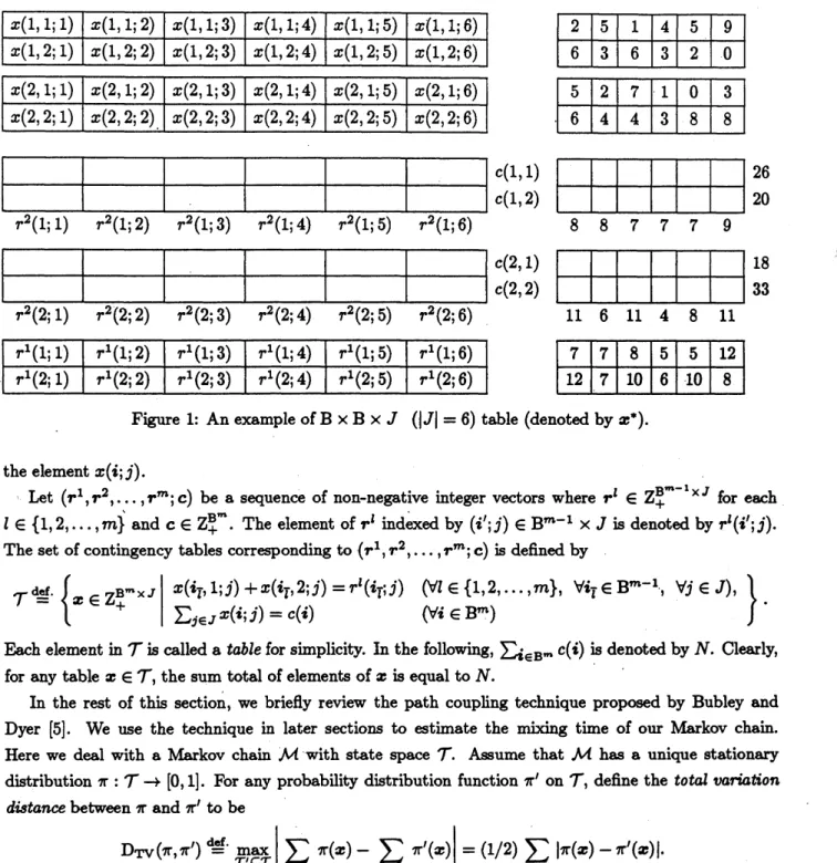
Figure 1: An exampleof$\mathrm{B}\mathrm{x}\mathrm{B}\mathrm{x}J(|J|=6)$table (denoted by $x^{*}$).
theelement $x(:;j)$
.
Let $(t^{1},r^{2}, \ldots,\mathrm{r}^{m};\mathrm{c})$ be asequence of non-negative integer vectors where $\Gamma^{l}\in \mathrm{Z}_{+}^{\mathrm{B}^{m-1}\mathrm{x}J}$ for each
$\mathit{1}\in\{1,2, \ldots,m\}\backslash$ and $\mathrm{c}\in \mathrm{Z}_{+}^{\mathrm{B}^{m}}$
.
The element of$\tau^{l}$ indexed by $(:\prime jj)\in \mathrm{B}^{m-1}\mathrm{x}J$ isdenoted by $r^{l}(:’;j)$
.
The set ofcontingency tables corresponding to $(T^{1}, r^{2}, \ldots,r^{m};\mathrm{c})$ is definedby$\mathcal{T}^{\mathrm{d}\mathrm{e}\mathrm{f}}=$.
$\{x$$\in \mathrm{Z}_{+}^{\mathrm{B}^{m}\mathrm{x}J}|x(\dot{\iota}_{7},1j)+x(i_{\overline{l}},2.j)=r^{l}(i_{\overline{l}},\cdot j)\sum_{j\in J}x(\dot{l}j)=c(\cdot)$ $(\forall l\in\{1,2, \ldots,m\}(\forall\dot{l}\in \mathrm{B}^{m})’\forall\dot{l}_{\overline{l}}\in \mathrm{B}^{m-1}, \forall j\in J)$
,
$\}$
.
Eachelement in$\mathcal{T}$is called atable forsimplicity. In the following, $\sum_{\in \mathrm{B}}$
.
$\mathrm{c}(\mathrm{i})$( isdenoted by$N$.
Clearly, for any table $x$ $\in \mathcal{T}$,
thesum
total ofelements of$isequal to $N$.
In the rest of this section, we briefly review the path coupling technique proposed by Bubley and Dyer [5]. We use the technique in later sections to estimate the mixing time of our Markov chain. Here we deal with aMarkov chain $\mathcal{M}$ with state space $\mathcal{T}$
.
Assume that $\mathcal{M}$ has aunique stationarydistribution $\pi$ : $\mathcal{T}arrow[0,1]$
.
For any probability distribution function $\pi’$on
$\mathcal{T}$,
definethe total variation distancebetween $\pi$and $\pi’$ to be$\mathrm{D}_{\mathrm{T}\mathrm{V}}(\pi,\pi’)=\mathrm{m}\mathrm{a}\mathrm{x}\mathrm{d}\mathrm{e}\mathrm{f}$. $\tau’\subseteq \mathcal{T}|\sum_{X\in \mathcal{T}},\pi(ax)-\sum_{l\in \mathcal{T}},\pi’(x)|=(1/2)\sum_{X\in \mathcal{T}}|\pi(x)-\pi’(ax)|$
.
If the initial state of the chain$\mathcal{M}$is$,wedenotethedistribution of the chain at time$t$by$P_{X}^{t}$:$\mathcal{T}arrow[0,1]$,
i.e.,
$P_{X}^{t}(y)=\mathrm{P}\mathrm{r}[X_{t}\mathrm{d}\mathrm{e}\mathrm{f}.=y|X_{0}=x]$ $(\forall y\in\eta$
.
Therate of convergence tostationaryfromthe initialstate $x$ may be measured by $\tau_{l}(\epsilon)=\min$
{
$\mathrm{d}\mathrm{e}\mathrm{f}$
.
$t|\mathrm{D}_{\mathrm{T}\mathrm{V}}(\pi,P_{X}^{t})\square \epsilon$ for all $t’\geq t$
}
where the
error
bound$\epsilon$ is agivenpositive constant. The mixing time$\tau(\epsilon)$ of$\mathcal{M}$is definedby$\tau(\epsilon)=\max\tau_{X}(\epsilon)\mathrm{d}\mathrm{e}\mathrm{f}.$, $ax\epsilon\tau$
which is independent of the initial state.
Next,
we
define aspecial Markov process with respect to $\mathcal{M}$ called joint process. Ajointprocess
of $\mathcal{M}$ isaMarkov chain $(X_{t},\mathrm{Y}_{t})$ defined on$\mathcal{T}\mathrm{x}\mathcal{T}$satisfying that eachof$(X_{t})$,$(\mathrm{Y}_{t})$, considered marginally,is afaithful copy of the original Markov chain$\mathcal{M}$
.
More precisely, werequirethat$\mathrm{P}\mathrm{r}[X_{t+1}=x’|(X_{t},\mathrm{Y}_{t})=(x, y)]$ $=$ $P_{\mathcal{M}}(x, ox’)$, $\mathrm{P}\mathrm{r}[\mathrm{Y}_{t+1}=y’|(X_{t},\mathrm{Y}_{t})=(x, y)]$ $=$ $P_{\mathcal{M}}(y,y’)$,
for all $x$,$y$,$\mathrm{x}$
’
$,$
$\in \mathcal{T}$where $P_{\mathrm{J}4}(x, x’)$ and $P_{\Lambda 4}(y,y’)$ denotes the transition probability from $x$ to $x’$
and from$y$ to$y’$ ofthe original Markov chain$\mathcal{M}$, respectively. Path coupling lemma [Bubley and Dyer [5]]
Let $G$be adirected graphwithvertex set $\mathcal{T}$and
arc
set$A\subseteq \mathcal{T}\mathrm{x}\mathcal{T}$.
Let $\ell:Aarrow \mathrm{Z}_{++}$ beapositivelength defined on the
arc
set. Weassume
that $G$is stronglyconnected. For anyordered pair ofvertices
$(x, x’)$ of$G$
,
the distance ffom $x$ to$x’$, denoted by $\ell(x, x’)$, isthe length ofthe shortest path from $x$to$x’$, where the length of apath isthe sumof the lengths of
arcs
inthe path. Suppose that thereexistsa
jointprocess $(X,\mathrm{Y})|arrow(X’,\mathrm{Y}’)$withrespectto$\mathcal{M}$ satisfyingthat$1>\exists\beta>0$, $\forall(X,\mathrm{Y})\in A$, $\mathrm{E}[\ell(X’,\mathrm{Y}’)]\square \beta\ell(X,\mathrm{Y})$
.
Then the mixing time$\tau(\epsilon)$ of the original Markov chain $\mathcal{M}$ satisfies $\mathrm{r}(\mathrm{e})\square (1-\beta)^{-1}\mathrm{h}(D/\epsilon)$where
$D$
denotes the diameter of$G$, i.e., the distance of afarthest (ordered) pair of vertices.
3Markov Chain for Uniform Distribution
First,
we
show alemma which impliesan irreducible Markovchain defined on the set of tables $\mathcal{T}$.
Wedefinethe paity
function
$\mathrm{p}:\mathrm{Z}arrow\{1, -1\}$by$\mathrm{p}(x)=\{$
1($x$ isan even integer),
-1 ($x$ is anodd integer ).
For anyindex$:\in \mathrm{B}^{m}$, we denote $\mathrm{p}(i_{1}+i_{2}+\cdots+i_{m})$ by$\mathrm{p}(:)$
.
The vector $\Delta\in\{1, -1\}^{\mathrm{B}^{m}}$ is definedby$\Delta(i)=\mathrm{p}(i)\mathrm{d}\mathrm{e}\mathrm{f}$.for each index$i\in \mathrm{B}^{m}$
.
Givenanordered pair of distinct column indices $(j’,j’)$,we definethe vector$\Delta[j’,j’]\in \mathrm{Z}^{\mathrm{B}^{m}\mathrm{x}J}$by
$\Delta[j’,j^{l/}](j)=\mathrm{d}\mathrm{e}\mathrm{f}$. $\{$
0 $(j\in J\backslash \{j’,j’\})$
,
$\Delta$ $(j=j’)$,
$-\Delta$ $(j=j’)$
.
Foranytable $x$ $\in \mathcal{T}$, we introducethe set ofneighboringtables;
$\mathrm{N}^{0}(x)\mathrm{e}=\{x’\in \mathcal{T}|\mathrm{d}\mathrm{f}.\exists(j’,j’)\in J\cross J, j’\neq j’, x’=x +\Delta[j’,j’]\}$
.
It is easy to see that if $x’=x$ $+.\mathrm{A}[\mathrm{j}’,\mathrm{j}"]$, then $x$ $=x’-\Delta \mathrm{b}’.,j’$] $=x’+\Delta[j’,j’]$, and
so
$x’\in$$\mathrm{N}^{0}(x)$ implies $x$ $\in \mathrm{N}^{0}(x^{j})$
.
For any pair of vectors $x$,$x’\in \mathrm{z}^{\mathrm{B}^{m}\mathrm{x}J}$,
$||x-x’||_{1}$ denotes the distance$\mathrm{I}$ $|x(:;j)-x’(:;j)|$ between$x$ and$x’$
.
$(:_{i})\in \mathrm{B}^{m}\mathrm{x}J$Figure 2: The vector $\Delta[4,2]$
.
Lemma 1Let $\sigma$ bean
undirected graph with vertex set$\mathcal{T}$ andfor
any pairof
vertices $\{x, ax’\}$, there existsan
edge between$x$ and$x’$if
and onlyif
$x’\in \mathrm{N}^{0}(x)$.
Then the graph$G^{0}$ is connected,:.
$e.$
,
for
anypair
of
vertices$\{x, x’\}$of
$G^{0}$,
there exists $\dot{a}$pathon
$\sigma$ between$x$ anti$x’$
.
The diameter (the distanceof
farthest
pairof
vertices) is less than orequal to$N/2^{m+1}$Proof. Assume
on
the contrary that $G^{0}$ is not connected. Let $\{x, x’\}$ be apair of vertices whichminimizes $||x-x’||_{1}$ subject to the condition that there does not exist any path between $x$ and $ox’$
.
Without lossof generality, we
can
assumethat $\exists j’\in J$, $\mathrm{x}(\mathrm{i};\mathrm{j}\mathrm{f})<d(2;j’)$,
where 2is the all-two vectorin Bm. It directly implies the followings;
1. $\mathrm{x}(\mathrm{i};\mathrm{j}\mathrm{f})<x’(i;j’)$ for any$:\in \mathrm{B}^{m}$satisfying $\mathrm{p}(i)=\mathrm{p}(\mathrm{i})$
,
2. $\mathrm{x}(\mathrm{i};\mathrm{j}\mathrm{f})>x’(i;j’)$ for any$i\in \mathrm{B}^{m}$satisfying $\mathrm{p}(i)\neq \mathrm{p}(\mathrm{i})$,3. $|x(:;j’)-x’(:;j’)|=|x(2;j’)-x’(2;j’)|$ for any$:\in \mathrm{B}^{m}$
.
Since
$\sum_{j\in J}x(2;j)=\sum_{j\in J}x’(2;j)$, thereexists acolumn index$j’$ satisfying$x(2;j’)>\mathrm{z}’(2,\mathrm{j}")$.
Thenwe have the followingproperties;
1. $\mathrm{x}(\mathrm{i};\mathrm{j}\mathrm{f})>x’(:;j’)$ for any$i\in \mathrm{B}^{m}$satisfying$\mathrm{p}(\mathrm{i})=\mathrm{p}(\mathrm{i})$,
2. $\mathrm{x}(\mathrm{i};\mathrm{j}\mathrm{f})<x’(:;j’)$ for any$i\in \mathrm{B}^{m}$ satisfying$\mathrm{p}(:)\neq \mathrm{p}(\mathrm{i})$,
3.
$|x(\dot{\iota};j’)-x’(i;j’)|=|x(2;j’)-x’(2;j’)|$ for any $:\in \mathrm{B}^{m}$.
The vector $x’=x$$+\mathrm{A}[\mathrm{j}\mathrm{f},\mathrm{j}"]$ is non-negative and so $x’\in \mathcal{T}$
.
Since $x’\in \mathrm{N}^{0}(x)$, there does not existanypath between $x’$and $x’$
.
The inequality $||x-x’||_{1}>||x’-x’||_{1}$ contradictswith the minimalityof$||x-x’||_{1}$
.
The definition of$x’$ implies that $||x-x’||_{1}=2^{m+1}$.
The above procedure decreases the distance between adistinct pair ofverticesand the decrement is
$2^{m+1}$
.
Ifwe
applythe procedure $\lfloor||x-x’||_{1}/2^{m+1}\rfloor$ times, the distance of twovertices isless than$2^{m+1}$.
It implies that the obtained pair of vertices are identical. Thus the diameter of$\sigma$ is less thanor equal
to$N/2^{m+1}$
.
$\square$The above lemma indicates theexistenceofan irreducible Markov chain
on
$\mathcal{T}$such that thetransition probability ofan ordered pair of tables $(x, x’)$ is positive if and only if $x$ and $x’$ are adjacent on $\sigma$.
When$m=1$,this chainisaspecialcaseof the Markov chain proposed byDiaconisand
Saloff-Coste
[10].However as discussed inDyer and’Greenhill [12], the mixing rate of Diaconis and Saloff-Coste’schainis
low. In the following, we describe our chain,which is an extension ofthe chain discussedby Dyer and
Greenhill [12] for contingencytableswithtworows
For any table $x\in \mathcal{T}$ and any pair ofdistinct column indices $\{j’,j’\}$, we define the following set of
tables;
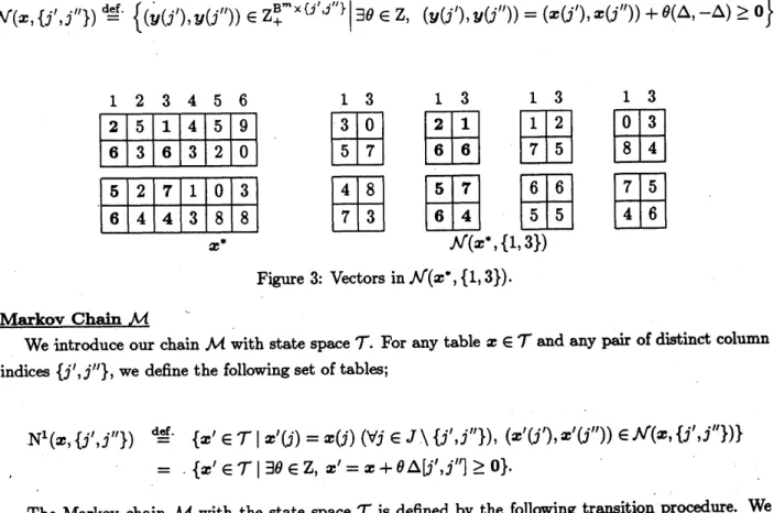
$N(x, \{j’,j’\})=\mathrm{d}\mathrm{e}\mathrm{f}$. $\{(y.(j’),y(j’))\in \mathrm{Z}_{+}^{\mathrm{B}^{m}\mathrm{x}\{j’,j’\}}|\exists\theta\in \mathrm{Z}$, $(y(j’), y(j’))=(x(j’), x(j’))+\theta(\Delta, -\Delta)\geq 0\}$
.
13131313
$35$ $07$ $62$ $61$ $\mathrm{f}_{7}^{1}\mathrm{f}_{5}^{2}1$ $08$ $43$ $47$ $83$ $65$ $47$ $\mathrm{f}_{5}^{6}\mathrm{f}_{5}^{6}1$ $47$ $65$ $N(x^{*}, \{1,3\})$ 30
5 7 2 1 6 60 3
8
4 48
73
5 7 6 4 75
46
Figure3:
Vectors in$N(x^{*}, \{1,3\})$.
$\mathrm{c}$ Markov Chain $\mathcal{M}$Weintroduce our chain$\mathcal{M}$with state space$\mathcal{T}$
.
For any table $x$ $\in \mathcal{T}$and any pair of distinct columnindices $\{j’,j’\}$, we define thefollowingset oftables;
$\mathrm{N}^{1}$(
$x$,$\{j’,j’\}$) $\mathrm{d}\mathrm{e}\mathrm{f}=$.
$\{x’\in \mathcal{T}$$|x’(j)=x(j)$ $(\forall j\in J\backslash \{j’,j’\})$, $(x’(j’),$ $ax’(j’))\in N(x$
,
$\{j’,j’\})\}$$=$ $\{x’\in \mathcal{T}|\exists\theta\in \mathrm{Z}, x’=ox +\theta\Delta[j’,j’]\geq 0\}$
.
The Markov chain $\mathcal{M}$ with the state space $\mathcal{T}$ is defined by the followingtransition procedure. We
denote the state ofthe chain $\mathcal{M}$ at time $t$ by $X_{t}$ and the element of$X_{t}$ indexed by $($
:;
$j)$ isdenotedby$X_{t}(i;j)$
.
Then the state $X_{t+1}$ at time $t+1$ is determined as follows. First, choose apair of distinctcolumn indices $\{\mathrm{j}’,\mathrm{j}"\}$ randomly. Next, choose atable $X_{t+1}$ from$\mathrm{N}^{1}(X_{t}|, \{j’,j’\})$ atrandom.
Figure 4: Theset of neighbors$\mathrm{N}^{1}$($’
,
{1,
3}).
We estimate the mixing time of
our
chain $\mathcal{M}$.
According to the definition, it is clear that $\mathcal{M}$ isaperiodic and irreducible. The transition probabilityof$\mathcal{M}$ from$x$ to $y$, denotedby $P_{\mathcal{M}}(x,y)$ is
$P_{\mathcal{M}}(x,y)=\{$
(
$(\begin{array}{l}n2\end{array})$ $|N(x, \{j’,j’\})|$)
( if$y\in \mathrm{N}^{1}(x;$$\{j’,j’\})$),
$\sum_{j’<j^{ll}}$
(
$(\begin{array}{l}n2\end{array})$ $|N(x, \{j’,j’\})|$)
$(x =y)$,0
(otherwise)Since
$P_{\Lambda 4}(x, y)=P_{\Lambda 4}(y,x)$, the stationarydistribution
of the chain is uniform.First,
we
introduce adirectedgraph$G$with the vertexset$\mathcal{T}$and thearc
set$A=\{(x, x’)|x’\in \mathrm{N}^{0}(x)\}$
.
We
define thatthe length $\ell(a)$ ofeacharc
$a\in A$isequalto 1. Thedistance ofany orderedpair of vertices$(x, x’)$on $G$isdenoted by$\ell(x,x’)$
.
Next, we defineajoint process $(X, \mathrm{Y})-\succ$ ($\mathrm{X}7$,Y7) with respect to$\mathcal{M}$.
For anypair of tables $(X, \mathrm{Y})\in A$, we definethe transition probability of
our
joint process from $(X,\mathrm{Y})$to $(X’,\mathrm{Y}’)$
.
Withoutlossof generality, we canassume
that$\mathrm{X}(1)\neq \mathrm{Y}(1),X(2)\neq \mathrm{Y}(2)$and$X(j)=\mathrm{Y}(j)$
forall$j\in J\backslash \{1,2\}$
.
In the joint process, we choose apair of distinct column indices $(j’,j’)$.
Case 1$\cdot$.
When$\{j’,j’\}\subseteq\{3, \ldots,n\}$, it is clear that$N(X, \{j’,j’\})=\mathrm{M}(\mathrm{Y}, \{j’,j’\})$ andso we choose a
pair $(Z(j’), Z(j’))$ ffom$N(X, \{j’,j’\})$ at random. Weset $X’$and $\mathrm{Y}’$ to the contingencytable obtained
from$X$and$\mathrm{Y}$by replacing $(X(j’),X(j’))$
and $(\mathrm{Y}(;7),\mathrm{Y}(\mathrm{j}"))$by $(Z(j’), Z(j’))$
, respectively.
Then, it isclear that $(X’,\mathrm{Y}’)$ is also
in
$A$andso
$\ell(X’,\mathrm{Y}’)=1$.
$\underline{\mathrm{C}\mathrm{a}\mathrm{e}\mathrm{e}2\cdot.}$Next, consider the
case
that $\{j’,j’\}=\{1,2\}$.
It is clear that$N(X, \{j’,j’\})=N(\mathrm{Y},\{j’,j’\})$
.
We construct $X’$and$\mathrm{Y}’$ byusing the
same manner
ofCase
1. Then, we have$X’=\mathrm{Y}’$ and$\ell(X’,\mathrm{Y}’)=0$
.
case$\mathrm{s}$ Finally,we consider thecase that$j’=1$ and$j’=3$
.
Other cases are treated in thesamewayas
follows.$\underline{\mathrm{C}\mathrm{a}\mathrm{e}\mathrm{e}3-1}$ Considerthecase that $\mu(X, \{j’,j’\})|=W(\mathrm{Y}, \{j’,j’’\})|$
.
Wedenote$\mathrm{N}^{1}(X, \{j’,j’\})=\{X^{1},X^{2}, \ldots,X^{k}\}$and$\mathrm{N}^{1}(\mathrm{Y}, \{j’,j’\})=\{\mathrm{Y}^{1},\mathrm{Y}^{2}, \ldots,\mathrm{Y}^{k}\}$
.
By arrangingtheorder of the elements,we
assume
that Xx$($1;$1)>X^{2}(1;1)>\cdots>X^{k}(1;1)$and$\mathrm{Y}^{1}(1;1)>\mathrm{Y}^{2}(1;1)>$$\ldots>\mathrm{Y}^{k}(1;1)$
.
Thenwechoose $(X’,\mathrm{Y}’)$ randomlyfrom$\{(X^{1},\mathrm{Y}^{1}), (X^{2},\mathrm{Y}^{2}), \ldots, (X^{k},\mathrm{Y}^{k})\}$.
It is easytosee
that $(X’,\mathrm{Y}’)\in A$andso$\ell(X’, \mathrm{Y}’)=1$.
iCase3-2
We
only need to consider thecase
that $|N(X, \{j’,j’\})|>\psi(\mathrm{Y}, \{j’,j’\})|$ without loss ofgenerality.
Since
$(X,\mathrm{Y})\in A$, it is easy toshow that $\mu(X,\{j’,j’\})|=|N(\mathrm{Y}, \{j’,j’\})|+1$.
Byarrangingthe order of elements in $\mathrm{N}^{1}(X, \{j’,j’\})=\{X^{1},X^{2}, \ldots,X^{k+1}\}$ and $\mathrm{N}^{1}(\mathrm{Y}, \{j’,j’\})=\{\mathrm{Y}^{1},\mathrm{Y}^{2}, \ldots, \mathrm{Y}^{k}\}$
,
we
can assume
that $\mathrm{X}(1)1)>X^{2}(1;1)>\cdots>X^{k+1}(1;1)$ and $\mathrm{Y}^{1}(1;1)>\mathrm{Y}^{2}(1;1)>\cdots>\mathrm{Y}^{k}(1;1)$.
Thenwe choose$(X’,\mathrm{Y}’)$ as follows;
$(X’,\mathrm{Y}’)=\{$
$(X^{t},\mathrm{Y}^{5})$ with probability $(k-i+1)/\mathrm{k}(\mathrm{k}+1)$ for $:\in\{1,2, \ldots,k\}$
,
$(X^{i+1},\mathrm{Y}‘)$ withprobability$i/k(k+1)$ for $i\in\{1,2, \ldots, k\}$,wherethe
sum
totalofthe probabilitiesis $(1+2+\cdots+k)/k(k+1)+(k+\cdots+2+1)/k(k+1)=1$.
Figure5shows
an
example. Clearly fromthe definition, $(X^{\ell},\mathrm{Y}^{t})$,
$(X^{t},\mathrm{Y}^{:+1})\in A$ foreach$:\in\{1,2, \ldots,k\}$ andso
$\ell(X’,\mathrm{Y}’)=1\backslash$
.
From the above,
we
have$\mathrm{E}[\ell(X’,\mathrm{Y}’)]=(1-$ $(\begin{array}{l}\mathrm{n}2\end{array}))$
.
It implies the following result.
$\tau(\epsilon)\square (1/2)n(n$-1)$\ln(dn/(2\epsilon))$, where d is the average
of
the values in celb,:.
e., d$=N/(2^{m}n)$.
$=\mathrm{Y}^{1}+\Delta[1,2]$ $=\mathrm{Y}^{2}+\Delta[1,2]$
$\mathrm{P}\mathrm{r}[(\mathrm{X}’,\mathrm{Y}’)=(X^{1},\mathrm{Y}^{1})|(j’,j’)=(1, 3)]=3/12$, $\mathrm{P}\mathrm{r}[(X’,\mathrm{Y}’)=(X^{2},\mathrm{Y}^{1})|(j’,j’)=(1,3)]=1/12$,
$\mathrm{P}\mathrm{r}[(\mathrm{X}’,\mathrm{Y}’)=(X^{2},\mathrm{Y}^{2})|(j’,j’)=(1,3)]=2/12$, $\mathrm{P}\mathrm{r}[(\mathrm{X}’,\mathrm{Y}’)=(X^{3},\mathrm{Y}^{2})|(j’,j’)=(1,3)]=2/12$, $\mathrm{P}\mathrm{r}[(\mathrm{X}’,\mathrm{Y}’) (X^{3},\mathrm{Y}^{3})|(j’,j’)=(1,3)]=1/12$, $\mathrm{P}\mathrm{r}[(X’,\mathrm{Y}’)=(X^{4},\mathrm{Y}^{3})|(j’,j’)=(1,3)]=3/12$
.
Figure 5: An exampleofCase
3-2.
$\mathrm{P}\mathrm{r}\mathrm{o}\mathrm{o}\dot{\mathrm{f}}$
.
The diameterofthe graph $G$is equal to that of$G^{0}$ and soless thanorequalto $N/2^{m+1}$.
Pathcoupling lemma induces the desired result. $\square$
Our chainisrapidly mixing. Moreover,
our
result indicates that the mixingtime independent of the dimension$m+1$ ofacontingency table in thecasethat the size is 2$\mathrm{x}2\mathrm{x}\cdots$ $\mathrm{x}J$.
4Discussion
In this paper,weproposedtheMarkovchainfor sampling2$\mathrm{x}2\mathrm{x}\cdots \mathrm{x}J$ contingency tables. Though the
author considered for constructing an efficient algorithm for finding all contingencytables, we couldn’t
propose it. With regard to enumeration algorithms for contingencytables, there are some results. $\mathrm{R}\triangleright$ cently, to enumerate
2-dimensional
contingency tables, Sturmfels proposed an algorithm using Grobner baseswhich arise fromalgebraic geometry [26]. Hisenumeration
algorithm is based onthereverse
searchtechnique. Sakata, SawaeandKroumovhave calculatedGrobner bases formonthsto
enumerate
4$\mathrm{x}4\mathrm{x}4$contingencytables [24]. Thusweneed to consider aboutpracticalalgorithms for enumerating contingency tables.
References
[1] A. Agresti, Asurveyof exact inference forcontingency tables,
Statistical
Science7(1992)131-153.
[2] A. Agresti, CategoricalData Analysis,JohnWiley&lSons,
2002
[3] D. Aldous, Random walks
on
finite groups and rapidly mixing Markovchains, in: A. Dold and B.Eckmann (Eds.), Seminaire de Probability XVII 1981/1982, vol.
986
of Springer-Verlag Lecture Notes inMathematics, Springer-Verlag, New York, (1983)243-297.
[4] S. AOKI AND A. TAKEMURA, Minimal basis for connected Markovchainover
3
x3xK’contingency
tables withfixed two dimensionalmarginals, Technical ReportMETR
2002-02
Dept. ofMathemat-ical Engineering and Information Physics, Faculty of Engineering, The University of Tokyo, 2002.
[5] R. Bubley and M. Dyer, Path coupling: Atechnique for proving rapid mixing in Markov chains,
38th Annual SymposiumonFoundations of ComputerScienceIEEE,San Alimitos, (1997) 223-231. [6]
R.
Bubley Randomized Algorithms :Approximation, Generation, and Counting, Springer-Verlag,New York,
2001.
[7] F.R.K. Chung,R.L. Graham, andS.T.Yau, Onsamplingwith Markovchains, RandomStructures
and Algorithms 9(1996) 55-77.
[8] P. Diaconis andB. Effron, Testing for independence in atwo way table: new interpretations of the
chi-square statistics (with discussion), Annals ofStatistics 13 (1985) 845-913.
[9] P. Diaconis and A. Gangolli, Rectangular arrays with fixed margins, in: D. Aldous, P. P. Varaiya,
J. Spencer, andJ. M. Steele (Eds.), IMA Volumes onMathematics anditsApplications, Springer,
New York,
72
(1995) $15\triangleleft 1$,
[10] P. Diaconis and L. Saloff-Coste, Random walk on contingency tables with fixed
row
andcolumn
sums,Technical Report, Department ofMathematics, Harvard University,
1995.
[11] P.Diaconis and B. Strumfels, Algebraic algorithms for sampling ffom conditionaldistributions, The Annals ofStatistics 26 (1998) $36\succ 397$
.
[12] NL Dyer andC. Greenhill, Polynomial-time countingand samplingof tw0-rowed contingencytables,
Theoretical ComputerSciences 246 (2000)
265-278.
[13] M. Dyer, R Kannan, and J. Mount, Sampling contingency tables, Random Structures and$\mathrm{A}\infty$
rithms
10
(1997)487-506.
[14] D. Edwards and T. Havranek, Afast procedure for model search in multidimensional cintingency
table, Biometrika
72
(1985)339-351.
[15] R. A. Fisher, StatisticalMethods for ResearchWorkers, Oliverand Boyde, Edinburgh,
1934.
[16] R.A. Fisher,The logic ofinductive inference (with discussion), Journalof RoyalStatisticalSociety
98
(1935) 39-54.[17] D.Hernek,Random generation of2
xn
contingencytables, RandomStructuresand Algorithms13(1998) 71-79.
[18] R. W.Irvingand M.R.Jerrum, Threedimensionalstatistical data security problems, SIAM Journal on Computing
23
(1994)170-184
[19] M. R. Jerrum and A. Sinclair, TheMarkov chain Monte Carlo method: anapproach toapproximate
countingandintegration, in Approximation Algorithm
for
$NP$-hard problems, D.S.Hochbaum (Ed.),PWS publishing, Boston, 1997, 482-520.
[20] M. Jerrum, A. Sinclair andE. Vigoda, Apolynomial-timeapproximation algorithm for the
perma-nent ofamatrixwith non-negative entries, in Proceedingsof the 33rd AnnualACMSymposium on
Theory ofComputing, ACMpress, NewYork,
2001712-721.
[21] R.Kannan,P. Tetali andS.Vempala, Simple Markov chain algorithm forgeneratingbipartite graphs
and tournaments, in 8th Annual Symposium on Discrete Algorithms, ACM-SIAM, San Francisco,
California,
1997193-200.
[22] C. R. Mehta and N. R. Patel, Anetwork algorithm for performing Fisher’s exact test in r
x
$c$contingencytables, Journal of the American Statistical Association78(1983)
427-434.
[23] K. Pearson,On the $\chi^{2}$test ofgoodness of fit, Biometrika 14 (1922)
186-191.
[24] T.SAKATA, R. SAWAEAND V. KROUMOV,ApplicationsofGrobnerBasisto Analysis of Contingency
Tables and IntegerProgramming, preprint,
2002.
[25] W. H. Sewell andA. M. Oewnstein, Communityof
residencial
and occupationalchoice, American journal of sociology70
(1965)551-563.
[26] B. STURMFELS, Grobner Bases andConvexPolytopes,UniversityLectureNotesSeries,8,American
MathematicalSociety,
1995.
[27] A. Takemura andS.Aoki,Some characterizationsofminimalMarkov basis for sampling from discrete conditional distributions TechnicalReport METR 2002-04,Dept. ofMathematicalEngineering and InformationPhysics, Facultyof Engineering, The UniversityofTokyo, 2002
![Figure 2: The vector $\Delta[4,2]$ .](https://thumb-ap.123doks.com/thumbv2/123deta/6026446.1066257/5.892.155.762.122.296/figure-the-vector-delta.webp)