PDF Fulltext | June 2016 Browse Articles 08 00555

(1)

Article

A Novel Combined Model Based on an Artificial

Intelligence Algorithm—A Case Study on Wind

Speed Forecasting in Penglai, China

Feiyu Zhang1_{, Yuqi Dong}2,_{* and Kequan Zhang}3

1 _{School of Statistics, Dongbei University of Finance and Economics, Dalian 116025, China;} [email protected]

2 _{School of Law, Guangxi Normal University, Guilin 541004, China}

3 _{Key Laboratory of Arid Climatic Change and Reducing Disaster of Gansu Province,}

College of Atmospheric Sciences, Lanzhou University, Lanzhou 730000, China; [email protected]

* Correspondence: [email protected] Academic Editor: Andrew Kusiak

Received: 12 April 2016; Accepted: 7 June 2016; Published: 14 June 2016

Abstract: Wind speed forecasting plays a key role in wind-related engineering studies and is important in the management of wind farms. Current forecasting models based on different optimization algorithms can be adapted to various wind speed time series data. However, these methodologies cannot aggregate different hybrid forecasting methods and take advantage of the component models. To avoid these limitations, we propose a novel combined forecasting model called SSA-PSO-DWCM, i.e., particle swarm optimization (PSO) determined weight coefficients model. This model consisted of three main steps: one is the decomposition of the original wind speed signals to discard the noise, the second is the parameter optimization of the forecasting method, and the last is the combination of different models in a nonlinear way. The proposed combined model is examined by forecasting the wind speed (10-min intervals) of wind turbine 5 located in the Penglai region of China. The simulations reveal that the proposed combined model demonstrates a more reliable forecast than the component forecasting engines and the traditional combined method, which is based on a linear method.

Keywords:sustainable energy; wind speed forecasting; optimization algorithm; combined model; weight coefficient optimization; de-noising procedure

1. Introduction

Due to increasing energy demands and environmental concerns, wind power has attracted global attention as a source of sustainable energy. China is rich in wind energy resources. According to one estimate of wind energy, at an altitude of 10 m, China has theoretical wind energy reserves of 600–1000 GW on land and offshore (exploitable) reserves of 100–200 GW. At present, the wind power industry is growing rapidly in the country [1]. It is well known that wind energy has three main weaknesses; low density, instability and regional variations. These features make wind speed difficult to predict. Wind speed forecasting can be summed up in three categories: ultra-short-term forecast, short-term forecast and mid-and-long term forecast [2]. In recent years, much research has been conducted to enhance wind speed forecasting accuracy, and these approaches can be divided into four categories: physical methods, statistical methods, hybrid physical-statistical approaches and artificial intelligence techniques [3]. Among these four categories, artificial intelligence techniques and statistical methods are the main methods studied in this paper.

Neural networks have good generalization ability, particularly in solving nonlinear problems, and they have been extensively used to forecast wind speed. Artificial Neural Networks (ANNs) have

(2)

Sustainability2016,8, 555 2 of 20

three advantages: first, they possess self-learning ability, second, ANNs have associative memory functions and, last, they are able to find optimal solutions. In the last 10 years, with the constant development of artificial neural networks, many researchers have proposed the application of artificial intelligence techniques to wind speed forecasting, including artificial neural and other mixed methods. A Wavelet Neural Network (WNN) is a typical and widely used artificial neural network due to its strong advantages in dealing with nonlinear estimation problems [4]. It has performed well in various fields, such as pattern recognition [5], image processing [6], forecast estimation [7], biology [8], medicine [9], economics [10] and others. The WNN method has several advantages such as high data error tolerance and no requirement for excess information beyond a wind speed history. It can fit unattained samples from historical data and can also approach an optimal nonlinear function with high precision. Based on the above advantages of WNNs, many studies have applied them to forecasting future data.

Decomposition of raw data is an important procedure for data filtering. It can effectively improve model forecasting precision and result in a better wind speed forecast [11]. Decomposition techniques such as Wavelet Decomposition (WD) [12] and Empirical Mode Decomposition (EMD) [13] are often employed to eliminate noise sequences. However, some limitations that need to be noted are that the WD method is sensitive to the threshold selection and the EMD method has an inherent disadvantage in the frequent appearance of mode mixing [14]. The de-noising method of singular spectrum analysis (SSA) used in this paper is somewhat different from de-noising techniques such as Fourier decomposition (FD) and wavelet decomposition (WD). It is one of the principal component analysis methods, which combine statistics and probability theory with concepts from dynamical systems and signal processing [15]. The main concept of SSA is that the original time series is decomposed into several components, which represent the trend, oscillatory behaviour (periodic or quasi-periodic components) and noise [16]. One of the strengths of the SSA technique compared with other non-parametric methods is that only two parameters are needed to reconstruct the original time series. SSA is often used to extract signals from one-dimensional short time sequences such as wind speed time series.

Individual artificial intelligence methods cannot always determine the link between each data point and obtain accurate forecasts [17]. To obtain better performance, hybrid forecasts have been presented using many approaches [18]. Hybrid forecasts have demonstrated significant improvement in forecasting results compared with using a single forecasting method [19]. Nevertheless, hybrid forecasting methods are based on just one or two optimization methods to improve individual models. It becomes uncertain whether the strengths of different optimization methods are fully exploited if more optimization methods are included. Thus, to avoid the above disadvantages, combination forecasts have been proposed as a novel method.

(3)

The primary contributions of this study are described as follows:

(1) A model based on the SSA de-noising technique is utilized to decompose wind speed time series and discard the noise. This procedure, by reducing the irregularity and instability of wind speed sequences, can improve model forecasting precision effectively.

(2) Each algorithm has its own advantages. On the basis of an analysis of the structure and parameters of a WNN, the CS (Cuckoo Search), PSO (Particle Swarm Optimization) and GA (Genetic Algorithm) algorithms can be employed to determine the number of wavelet nodes and related parameters such as initial values. These procedures give the optimized artificial neural network higher stability, convergence speed and prediction accuracy.

(3) A novel combined model, the SSA-PSO-DWCM, is developed for the wind-speed forecasting field that, for the first time, combines three hybrid models using an intelligent technique method. The combined model integrates the advantages of its component models and breaks through the limitations of traditional non-negative theory.

(4) Considering the randomness of the optimization method and the nonlinearity of the wind series, every experiment was performed 10 times to ensure the reliability of the conclusions.

This paper’s structure is as follows; Section2introduces the individual optimization theories (Cuckoo Search, Genetic Algorithm and Particle Swarm Optimization), the Wavelet Neural Network prediction method and the Singular Spectrum Analysis de-noising method. Section3proposes the combined approach. In Section4, to illustrate the effectiveness of the proposed SSA-PSO-DWCM combined model, several cases are simulated. Experimental design, results and discussion comprise this section. Finally, Section5gives a comprehensive summary of this study.

2. Forecasting Theory

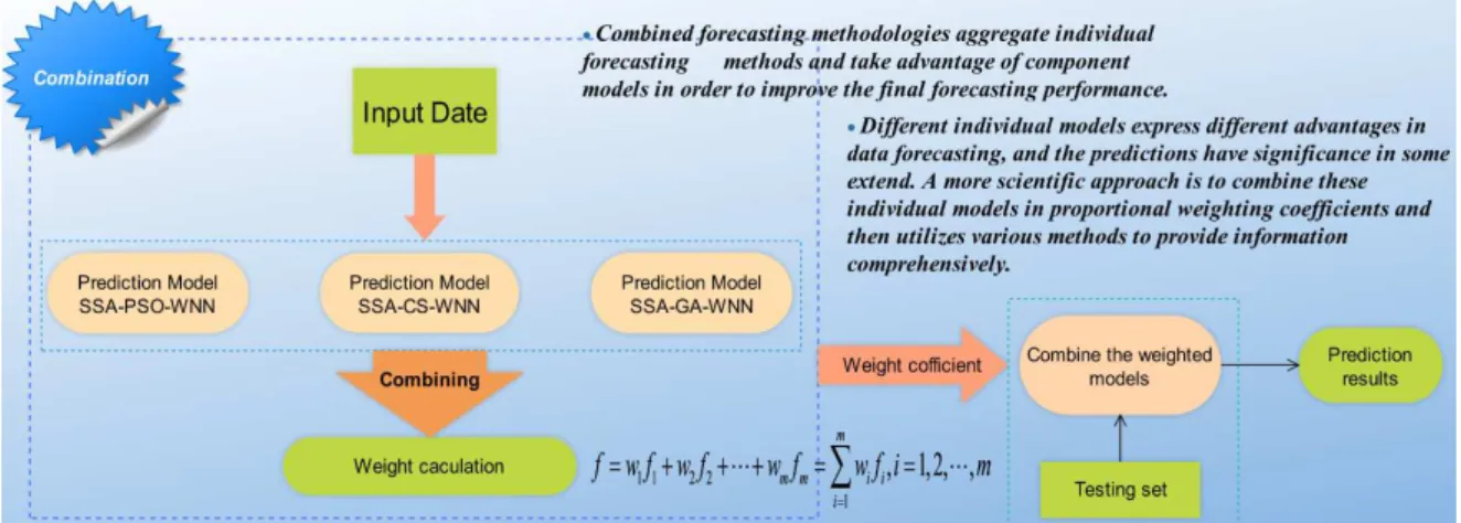
A combined model adopts advantage of its component models is superior to the individual models or performs at least as well as the best one, as has been proven by many simulation results [24]. This work proposes a novel combined method to forecast wind speed which includes three hybrid models: SSA-CS-WNN, SSA-GA-WNN and SSA-PSO-WNN. First, Singular Spectrum Analysis (SSA) is applied to decompose and reconstruct the raw wind sequence. Then, three hybrid models (SSA-CS-WNN, SSA-GA-WNN and SSA-PSO-WNN) are built to forecast wind speed. Finally, particle swarm optimization (PSO) is employed to determine the weighting coefficients of these three hybrid models, and a final combined model is proposed.

2.1. Cuckoo Search (CS) Algorithm

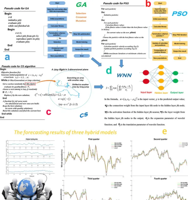
A cuckoo is a charming bird that makes a beautiful sound and has an aggressive reproduction strategy. Numerous studies have described that many insects and animals exhibit the behavior of Lévy flights [25]. A moving objective takes a stochastic step to alter the behavior of a system; this situation can be described as a Lévy flights; a sketch is shown in Figure1, part c.

(4)

‐ ‐

‐

Figure 1.Comprehensive presentation of three optimization algorithms and the forecasting method: (a) Genetic Algorithm pseudo-code and flowchart; (b) Particle Swarm Optimization pseudo-code and flowchart; (c) Cuckoo Search pseudo-code and flowchart; (d) structure of the WNN; (e) forecasting results of three hybrid models for four quarters.

Table 1.CS experimental parameters.

Experimental Parameters Default Value

CS the scale of bird’s nest 20

(5)

Table 2.GA parameters.

GA population scale 200

GA population scale 50

GA cross rate 0.8

GA mutation rate 0.05

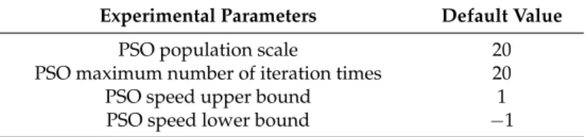
Table 3.PSO parameters.

PSO population scale 20

PSO maximum number of iteration times 20

PSO speed upper bound 1

PSO speed lower bound ´1

Table 4.WNN experimental parameters.

the number of the input nodes 6

the number of the hidden nodes 6

the number of the output nodes 1

the learning velocity 1 0.01

the learning velocity 2 0.001

iteration time 20

2.2. Genetic Algorithm (GA)

The genetic algorithm was proposed by Professor Holland of the University of Michigan in 1962 [26]. This algorithm operates on a number of potential solutions, applying the principle of survival of the fittest to produce better and better estimated values to a solution. Currently, genetic algorithms are used to optimize neural nets to solve some complicated problems [27]. The basic manipulations of GA contain six parts as described below [28].

Step 1: Generate the initial population in a random way. Step 2: Compute and save each individual’s fitness.

Step 3: Based on different fitness values, the selection procedure chooses an individual for a new group. The probability of being chosen is proportional to the individual fitness value. Step 4: A crossover operation is carried out by selecting two matching parents in which two random

places are selected on each chromosome string and the string segments between these two places are exchanged between the mates.

Step 5: Mutation randomly modifies elements in the chromosomes and is employed with low probability, typically from 0.001 to 0.01.

Step 6: If the above steps have not found optimal solutions,i.e., the minimum objective function value has not been obtained, the procedure goes back to Step 2.

In this paper, the simple genetic algorithm (SGA) which demonstrates the main principles of a GA in a simple way [29] is applied to sketch the primary properties of GA and the pseudo-code is shown in Figure1, part a. Table2illustrates the experimental parameters of the GA used in this study. 2.3. Particle Swarm Optimization (PSO) Algorithm

(6)

determined [30]. The purpose of the PSO algorithm is to look to the optimal solution of one problem [31]. This paper uses the pseudo-code demonstrated in Figure1, part b to describe the basic steps of the PSO algorithm. The experimental parameters of the PSO algorithm in this study are shown in Table3.

2.4. Wavelet Neural Network (WNN)

The wavelet neural network (WNN) is a network which is based on the structure of the BP neural network; Multiple-dimensions and feed-forward are characteristic of WNNs. The wavelet neural network method regards the wavelet basis function as the transfer function of the hidden layer nodes. The basic structure of WNN is a three-layer neural network which is shown in Figure1, part (d). There aremnodes in the input layer, while the hidden layer hasnwavelet bases and only one output. WNN not only converges quickly, but also can avoid local optima because of its strong learning and generation capacity [32]. The experimental parameters of WNN in this study are shown in Table4.

The structure of the wavelet neural network is always described by the following formula:

ˆ y“

n ÿ

t“1 wtyt

˜ _m ÿ

k“1

uktxk´bt at

¸

(1)

In the formula, ˆy is the final predicted value and has just one element; x “ px1,x2,¨ ¨ ¨ ,xmqT represents the initial input vector;uktis the weight of the connection from the input layerkth neuron to the hidden layertth neuron; the product ofwtandψtis the wavelet basis function;atis the stretch factor of the wavelet basis function andbtis the translation vector of the wavelet basis function. In this paper, the Morlet wavelet is adopted as an activation function in the hidden nodes because, in comparison to the broader Mexico hat wavelet, orthogonal wavelet, and Gauss spine wavelet, the Morlet wavelet has the smallest error and the best computational stability [33]. The formula is given below:

y“cosp1.75xqe´x2{2 (2)

2.5. Singular Spectrum Analysis (SSA)

Singular spectrum analysis (SSA) based on the dynamic reconfiguration of time series. It is a statistical technique associated with the empirical orthogonal function. It is often used for analyzing time series and extracting oscillatory components from the original data. SSA is often used to analyse one-dimensional time series of the formx1,x2,x3,¨ ¨ ¨,xN. The trajectory matrixYis constructed from the primitive sequenceXbased on a window of lengthL. The procedure of SSA is described below:

(1) Embedding. Arrange a lag and choose a favorable “window”Lp2ďLďN{2q. Build the trajectory matrix as below:

Y“

¨

˚ ˝

x1 ¨ ¨ ¨ xL ..

. . .. ... xN´L`1 ¨ ¨ ¨ xN

˛

‹

‚ (3)

(2) Calculate the covariance matrix Cof the trajectory matrix, with diagonals corresponding to equal lags:

C“

¨

˚ ˝

c0 . . . cL´1 ..

. . .. ... cL´1 ¨ ¨ ¨ c0

˛

‹

‚ (4)

(7)

(3) Divide the matrices into applicable groups and calculate the sum of each group after the decomposition procedure. The projection of lagged seriesYonEk:

aik“ M ÿ

j“1

xi`jEkj,p0ďiďN´L, 1ďjďLq (5)

aikis called the time principle component (TPC).

(4) The most important procedure of SSA is the component reconstruction. Two parameters, L (“window” length) and Y (the pattern of grouping the matrices), which are based on the attributes of the primitive sequences and the final analysis’ objective, are vital for the final decomposition result.

Reconstruction componentXk_i:

Xki “ $ ’ ’ ’ ’ ’ ’ ’ ’ & ’ ’ ’ ’ ’ ’ ’ ’ % 1 i i ř

j“1

ai´j`1,kEk,jp1ďiďL´1q

1 M

L ř

J“1

ai´j`1,kEk,jpLďiďm`1q

1 N´i`1

i ř

j“i´N`L

ai´j`1,kEk,jpN´L`2ďiďNq

(6)

SSA decomposes original data intomreconstructed series; the first reconstructed seriesX1is regarded as the most important one. Hence, the rest are discarded as noise.

2.6. The Hybrid Models SSA-CS-WNN, SSA-GA-WNN, and SSA-PSO-WNN

It is difficult for a single WNN desirable wind speed forecasting results, though the WNN is suitable for handling small samples or high-dimensional complex problems. What is worse, the irregularity and nonlinearity of wind speed data cause more difficulties in the wind speed prediction procedure. To address the shortcoming that an individual model cannot entirely integrate the information contained in real problem records, three optimization methodologies (CS, GA and PSO) are used to assign the number of wavelet nodes and related parameters such as initial values in this study. We use SSA to reconstruct the original series to obtain the de-noising sequences because it has been confirmed to be a promising method to extract the noise from the original wind speed series. The applied models’ results after the SSA de-noising procedure have a higher accuracy than the same models without the de-noising procedure.

3. Combined Model

Recent studies have predominantly focused on short-term wind speed forecasting ranging from minutes to hours because of the importance of these forecasts for power systems. Various attempts have been made to use hybrid methods for short-term wind forecasting. The combined approaches most commonly seen in the literature are data pre-processing-based approaches, parameter-optimization-based approaches and weighting-based approaches [34]. Combination forecasts can be used to enhance the eventual prediction results because they can integrate signal forecasting models and make use of component forecasts. Figure 2shows the flowchart for the weighting-based combined approaches. The main idea of the optimal mix forecasting method can be expressed as the following mathematical programming problem:

maxpminqQ“Qpw1,w2,¨ ¨ ¨,wmq (7)

(8)

‐ ‐    





















 

‐

x

‐

Figure 2.Flowchart for the weighting-based combined approach. 3.1. Traditional Combination Forecasting Theory (Weighting-Based Combined Approaches)

Different individual models have different advantages for data forecasting, and each forecast has some degree of significance. A more scientific approach is to combine these single models using proportional weighting coefficients and then to utilize various methods to provide comprehensive information. The traditional combination forecasting approach attempts to find the best weight for each of the combined models based on minimizing MAPE. In this study

minJ“LTEL“

T ÿ

t“1 m ÿ

j“1 m ÿ

i“1 liljeitejt

#

RTL“1

Lě0 (8)

whereL“ pl1,l2,¨ ¨ ¨,lmqTis the weight vector,R“ p1, 1,¨ ¨ ¨, 1qTis a column vector where all elements are 1 andEij “ eTi ej, whereei “ pei1,ei2,¨ ¨ ¨,eiNq. E “

` Eij

˘

mˆm is the error information matrix; Jrepresents the MAPE,et“xt´xˆt;eitis the error of theith method at timet; and ˆxtrepresents the forecast value of theith method at timet.

3.2. Artificial Intelligence Algorithms

In addition to the above traditional methods, an artificial intelligence optimization algorithm has been used in many approaches [35]. To find the optimal forecasts, this study proposed using the particle swarm optimization algorithm to determine the weighting coefficients. Combined forecasting models can also be divided into variable weight combination forecasting methods and invariable weight combination forecasting methods based on whether the weight changes over time. This paper based on the minimum mean absolute percentage error (MAPE), which belongs to the constant weight combination method. This section provides a weight-determined method that was assessed by experimental simulation rather than a theoretical proof.

After repeated experiments, it was found that the sum of the weights is not precisely equal to 1, it approximates that value. In addition, the weights may calculate a negative value. The amended method is expressed below:

minJ“LTEL“

T ÿ

t“1 m ÿ

j“1 m ÿ

i“1 liljeitejt

#

RTL«1

´1ďLď1 (9)

(9)

4. Experimental Design, Results and Discussion

In this section, several cases are presented to demonstrate the effectiveness of the proposed hybrid approach through comparisons with other models. These studies are presented in four sequential sections: data collection, forecast performance evaluation criteria, simulation forecast procedure and comparison and discussion.

4.1. Data Set

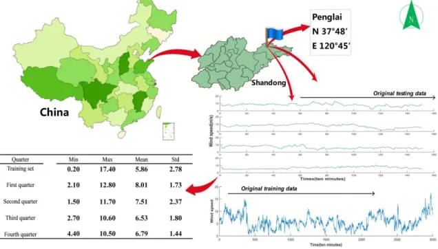
The proposed SSA-PSO-DWCM combined model was tested by forecasting the wind speed (in 10-min increments) of wind turbine 5 located in the Penglai region of China. A simple map of the study area is shown in Figure3. In this section, several studies are presented to illustrate the effectiveness of the proposed combined approach through comparisons with other models. To examine the stability of the combined method, we present our analysis of four days of data from four quarters. Because the wind speed time series includes some uncertainty and some parameters of the combined method have no defined value, we make the following assumptions:

(1) Due to the highly random nature of wind speed processes, the experimental data have been randomly selected from four quarters, and the experimental results are regarded as general results. (2) For ease of plotting, T (the period of the time series) is 144.

‐

 ‐





 ‐



 ‐

y

‐

Figure 3.Location of Penglai wind farm in China and statistical properties of the original data.

(10)

Sustainability2016,8, 555 10 of 20      







‐

‐ ‐ ‐ ‐ ‐ ‐ ‐ ‐ ‐ ‐ ‐ ,

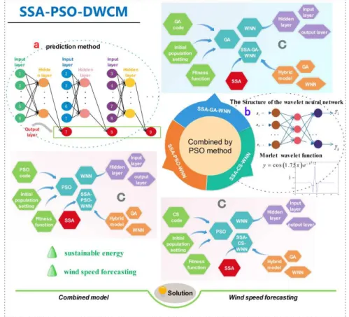
Figure 4.Flowchart of the combined model SSA-PSO-DWCM: (a) a brief illustration of the prediction method; (b) structure of the WNN and image of the Morlet wavelet function; (c) three hybrid models: SSA-PSO-WNN, SSA-GA-WNN and SSA-CS-WNN.

4.2. Evaluation Indices for Forecasting Performance

Many performance measures have been applied in previous approaches to evaluate the forecast accuracy, but no one single measure can be regarded as the common estimation criterion. For the above reason, we should select several representative indicators to evaluate the quality of these algorithms. In this paper, three evaluation criteria are used: mean absolute error (MAE), Equation (10); mean square error (MSE), Equation (11); and mean absolute percentage error (MAPE), Equation (12).

MAE“ _N1

N ÿ

n“1

|yi´yˆi| (10)

MSE“ 1

N N ÿ

n“1

pyi´yˆiq 2

(11)

MAPE“_N1

N ÿ

n“1 ˇ ˇ ˇ ˇ

yi´yˆi yi ˇ ˇ ˇ ˇˆ 100% (12)

In the above formulas,Nis the scale of the test data; ˆyirepresents the forecast result for time periodi, whereasyirepresents the actual wind speed for the same time period. Out of these three criteria, MAPE is regarded as the main estimation index in this paper because it is a unit-free measure of accuracy for the predicted wind series and is sensitive to small changes in the data.

(11)

4.3. Forecasting Procedure

This paper employs 3000 samples ranging from 00:10 on 6 June to 20:00 on 26 June 2011 to simulate the models and regards the raw data of the Penglai region as a random series. Then, the models are employed to forecast the wind speed for four different days drawn from four different quarters. The experimental process consisted of several steps as follows:

Step 1: Execute Wavelet Neural Network (WNN) method forecasts and collect the results (for four quarters of wind turbine 5).

Step 2: Run three hybrid models PSO-WNN, CS-WNN and GA-WNN to forecast wind speed. Step 3: Combine the three hybrid forecast models by using the traditional combination method. Step 4: Combine the three hybrid forecast models based on the PSO-determined weighting

coefficient method.

Step 5: Use SSA to filter the raw wind speed data to decrease its non-stationarity. Then, use the de-noised data to rerun the models following the above Steps 1–4. The flowchart of the combined method SSA-PSO-DWCM is shown in Figure4.

4.4. Analysis of Forecast Results and Comparisons of Different Models

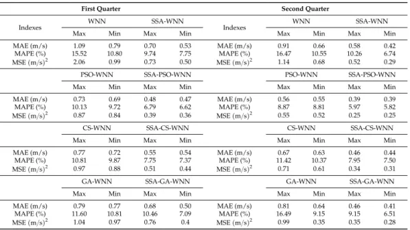
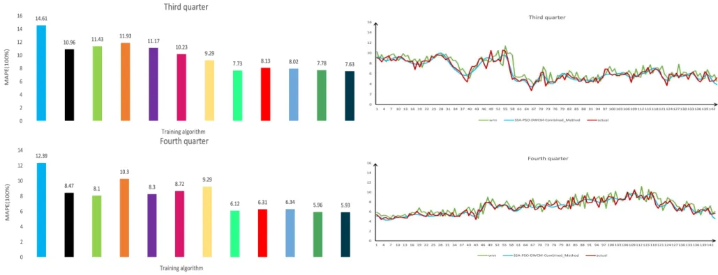
Considering the randomness of the optimization methods, each program was executed 10 times. The maximum and minimum values of the indexes for each quarter and all experiments are presented in Tables5and6. To facilitate the analysis and discussion of the proposed combined model, 10 other models for short-term wind speed forecasting are employed for comparison and assessment of the prediction performance in this subsection. From the first quarter’s simulation results, we can conclude that the single WNN shows the largest fluctuation and the highest MAPE, which ranges from 15.52% to 10.80%. After combining the three optimization algorithms, the MAPE becomes more steady and decreases to some extent. The PSO-WNN ranges from 10.13% to 9.72%, CS-WNN ranges from 10.81% to 9.87%, and GA-WNN ranges from 16.49% to 10.81%. In SSA-WNN, SSA-PSO-WNN, SSA-CS-WNN and SSA-GA-WNN models, the MAPE decreased significantly. The three hybrid models’ forecast results for four quarters are highlighted in Figure1, part e. The final forecasting results illustrate that decomposing the raw wind speed signals by SSA can not only improve the forecasting accuracy but can also lower the fluctuation of the MAPE. The above conclusions can also be drawn from the results for the other quarters in Tables5and6.

Table 5.Maximum and minimum index values for the first and second quarters in all cases. First Quarter Second Quarter

Indexes WNN SSA-WNN Indexes WNN SSA-WNN

Max Min Max Min Max Min Max Min

MAE (m/s) 1.09 0.79 0.70 0.53 MAE (m/s) 0.91 0.66 0.58 0.42

MAPE (%) 15.52 10.80 9.74 7.75 MAPE (%) 16.47 10.55 10.26 6.74

MSEpm{sq2 2.06 0.99 0.73 0.50 MSEpm{sq2 1.14 0.68 0.52 0.29

PSO-WNN SSA-PSO-WNN PSO-WNN SSA-PSO-WNN

MAE (m/s) 0.73 0.69 0.48 0.47 MAE (m/s) 0.56 0.55 0.39 0.39

MAPE (%) 10.13 9.72 6.79 6.62 MAPE (%) 8.87 8.81 5.97 5.82

MSEpm{sq2 0.87 0.84 0.39 0.36 MSEpm{sq2 0.55 0.52 0.25 0.25

CS-WNN SSA-CS-WNN CS-WNN SSA-CS-WNN

MAE (m/s) 0.77 0.72 0.55 0.54 MAE (m/s) 0.67 0.63 0.46 0.44

MAPE (%) 10.81 9.87 7.75 7.37 MAPE (%) 11.42 10.37 7.95 7.50

MSEpm{sq2 0.97 0.88 0.51 0.44 MSEpm{sq2 0.71 0.61 0.34 0.31

GA-WNN SSA-GA-WNN GA-WNN SSA-GA-WNN

MAE (m/s) 0.79 0.77 0.68 0.50 MAE (m/s) 0.81 0.64 0.46 0.41

MAPE (%) 11.60 10.81 10.46 7.09 MAPE (%) 16.49 9.15 9.15 6.51

(12)

Table 6.Maximum and minimum index values for the third and fourth quarters in all cases.

Third Quarter Fourth Quarter

Indexes WNN SSA-WNN Indexes WNN SSA-WNN

MAE (m/s) 0.97 0.65 0.5920 0.4837 MAE (m/s) 0.94 0.74 0.63 0.43 MAPE (%) 16.46 11.10 10.19 7.97 MAPE (%) 13.37 10.65 10.08 6.27 MSEpm{sq2 _1.56 _0.71 _0.56 _0.37 _MSE_p_m_{_s_q2 _1.45 _0.83 _0.57 _0.30

PSO-WNN SSA-PSO-WNN PSO-WNN SSA-PSO-WNN

MAE (m/s) 0.64 0.62 0.46 0.46 MAE (m/s) 0.59 0.57 0.42 0.41 MAPE (%) 10.96 10.61 7.83 7.73 MAPE (%) 8.75 8.47 6.12 5.93 MSEpm{sq2 0.71 0.68 0.35 0.35 MSEpm{sq2 0.56 0.52 0.27 0.27

CS-WNN SSA-CS-WNN CS-WNN SSA-CS-WNN

GA-WNN SSA-GA-WNN GA-WNN SSA-GA-WNN

4.4.1. Forecast Results without De-Noising Procedure

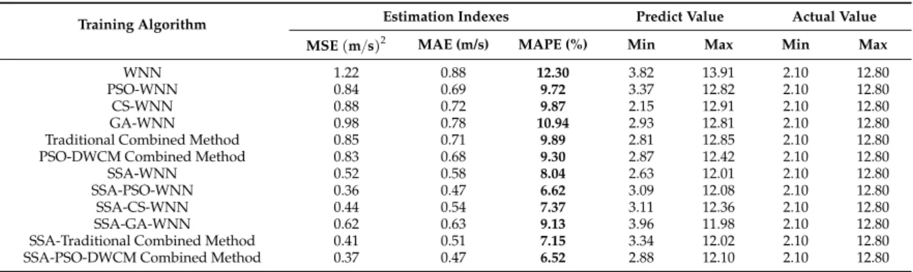
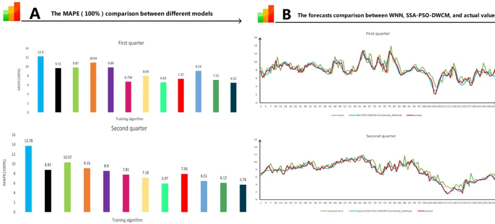
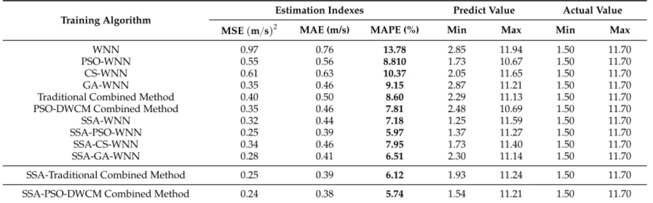
The evaluation index results for different forecasting methods are compared in Tables7–10; the first six rows of these four tables present the forecasts without decomposition. MAE, MSE and MAPE are used to monitor the forecasting accuracy. Wind speed in every quarter was forecast using 10 models to compare the forecasting accuracy; comparisons of MAPE for different models are shown in Figure5, part a. From the first six rows of Tables7–10, we can see that the individual WNN has the lowest accuracy, better performance is provided by the three hybrid optimization models PSO-WNN, CS-WMN and GA-WNN. However, we find that the forecasting accuracy of the Traditional Combined Method is low compared with the three hybrid optimization models. This situation occurs because the Traditional Combined Method cannot integrate all of the advantages of the hybrid models. In Table7, the MAPE of the PSO-DWCM model is 9.30%, which is 3.00%, 0.42%, 0.57% and 1.64% lower than the WNN, PSO-WNN, CS-WNN and GA-WNN models, respectively. These data indicate that the PSO-DWCM is a viable method to exploit the advantages of different models. The other three quarters also support the above conclusions.

Table 7.Evaluation indices of different models in the first quarter for wind turbine 5.

Training Algorithm Estimation Indexes Predict Value Actual Value

MSEpm{sq2 MAE (m/s) MAPE (%) Min Max Min Max

WNN 1.22 0.88 12.30 3.82 13.91 2.10 12.80

PSO-WNN 0.84 0.69 9.72 3.37 12.82 2.10 12.80

CS-WNN 0.88 0.72 9.87 2.15 12.91 2.10 12.80

GA-WNN 0.98 0.78 10.94 2.93 12.81 2.10 12.80

Traditional Combined Method 0.85 0.71 9.89 2.81 12.85 2.10 12.80 PSO-DWCM Combined Method 0.83 0.68 9.30 2.87 12.42 2.10 12.80

SSA-WNN 0.52 0.58 8.04 2.63 12.01 2.10 12.80

SSA-PSO-WNN 0.36 0.47 6.62 3.09 12.08 2.10 12.80

SSA-CS-WNN 0.44 0.54 7.37 3.11 12.36 2.10 12.80

SSA-GA-WNN 0.62 0.63 9.13 3.96 11.98 2.10 12.80

(13)

(14)

‐

‐ ‐ ‐ ‐ ‐ ‐ ‐ ‐ ‐ ‐ ‐ ‐ ‐ ‐ ‐

(15)

Table 8.Evaluation indices of different models in the second quarter for wind turbine 5.

WNN 0.97 0.76 13.78 2.85 11.94 1.50 11.70

PSO-WNN 0.55 0.56 8.810 1.73 10.67 1.50 11.70

CS-WNN 0.61 0.63 10.37 2.05 11.65 1.50 11.70

GA-WNN 0.35 0.46 9.15 2.87 11.21 1.50 11.70

SSA-WNN 0.32 0.44 7.18 1.25 11.59 1.50 11.70

SSA-PSO-WNN 0.25 0.39 5.97 1.37 11.27 1.50 11.70

SSA-CS-WNN 0.34 0.46 7.95 1.73 11.40 1.50 11.70

SSA-GA-WNN 0.28 0.41 6.51 2.30 11.14 1.50 11.70

SSA-Traditional Combined Method 0.25 0.39 6.12 1.93 11.24 1.50 11.70 SSA-PSO-DWCM Combined Method 0.24 0.38 5.74 1.54 11.21 1.50 11.70

Table 9.Evaluation indices of different models in the third quarter for wind turbine 5.

WNN 1.24 0.84 14.61 3.7 11.40 2.70 10.60

PSO-WNN 0.71 0.64 10.96 3.05 10.24 2.70 10.60

CS-WNN 0.74 0.67 11.43 2.97 9.70 2.70 10.60

GA-WNN 0.81 0.70 11.93 3.46 10.95 2.70 10.60

SSA-WNN 0.50 0.54 9.29 3.29 10.27 2.70 10.60

SSA-PSO-WNN 0.34 0.46 7.73 3.54 10.03 2.70 10.60

SSA-CS-WNN 0.38 0.48 8.13 2.86 9.84 2.70 10.60

SSA-GA-WNN 0.47 0.37 8.02 3.50 10.06 2.70 10.60

Table 10.Evaluation indices of different models in the fourth quarter for wind turbine 5.

WNN 1.07 0.83 12.39 4.58 11.22 4.40 10.50

PSO-WNN 0.53 0.57 8.47 4.45 9.12 4.40 10.50

CS-WNN 0.53 0.56 8.10 4.27 9.53 4.40 10.50

GA-WNN 0.74 0.69 10.30 4.85 10.84 4.40 10.50

SSA-WNN 0.55 0.58 9.29 4.06 9.99 4.40 10.50

SSA-PSO-WNN 0.27 0.42 6.12 4.21 9.77 4.40 10.50

SSA-CS-WNN 0.30 0.43 6.31 4.18 9.63 4.40 10.50

SSA-GA-WNN 0.28 0.42 6.34 4.22 9.69 4.40 10.50

4.4.2. Forecast Results with SSA De-Noising Procedure

(16)

Relative Error (RE) Equation (14) and the Root Mean Square Error (RMSE) Equation (15) to measure the deviation between the observed values and the true values. Larger R and smaller RE and RMSE indicate a similar connection between the de-noised data and the original data.

R“ covpyt,yq

σytσy

(13)

RE“|y´yt|

y (14)

RMSE“

g f f e1

N N ÿ

i“1

pyt´yq2 (15)

where yt and y represent the de-noising data and the original data, respectively, covpyt,yqis the covariance between ytandy.σytandσyrepresent the variance ofytandy, respectively.

Train

ing

proc

ess

Forecasting

re

su

lt

s

‐

‐ ‐

‐ ‐ ‐

‐ ‐

Figure 6.First quarter forecasting results obtained using SSA.

(17)

Table 11.Correlation index between the de-noise data and the original data.

Quarter Data Set Correlate Index

Original De-Noising R RE (100%) RMSE (100%)

First quarter 3150 3150 0.9849 0.58% 0.42%

Second quarter 3150 3150 0.9846 0.60% 0.42%

Third quarter 3150 3150 0.9841 0.61% 0.41%

Fourth quarter 3150 3150 0.9844 0.59% 0.42%

Rows 7–12 of Tables7–10represent the forecasts obtained using the decomposed samples. It clearly shows that the models reconstructed by SSA perform better than the models using the original data. The largest improvement in forecasting accuracy is determined by the de-noising procedure. Finally, the MAPE of the SSA-PSO-DWCM method in the first quarter is 6.52%, which is a decrease of 5.78% compared to the single model WNN. This value illustrates a great reduction in forecasting accuracy. The simulation results for the other three quarters also support the above views. Furthermore, SSA-PSO-DWCM shows stronger forecasting capability compared to the SSA-Traditional combined method, because the novel combination method is more reasonable, more scientific, and more applicable to practical problems than no negative constraint theory combination models. A comparison of forecasting results between WNN and SSA-PSO-DWCM for four quarters is shown in Figure5, part (b). 4.4.3. Analysis of Different Weighting Coefficients

In this paper, the traditional method and the PSO optimization method are employed to optimize the weighting coefficients. Different hybrid models’ weighting coefficients were calculated according to different weighting coefficient determination methods and the results are shown in Table12. We can conclude that the weighting coefficients determined by the traditional combined method have two characteristics: the sum of the three weights is equal to the value 1 and each of the weighting coefficients is larger than 0. In contrast, the sum of these three weighting coefficients when optimized by the artificial intelligence algorithm PSO is close to 1 and the weighting coefficients range from´1 to 1. The results illustrate that the intelligence algorithm PSO can enlarge advantages and avoid drawbacks in an effective way to estimate the performance of different models.

Table 12.Different weighting coefficients determined by traditional method and PSO method.

Quarter Weighting Coefficients Determined Method Hybrid Models’ Weighting Coefficients

First quarter

PS0-WNN CS-WNN GA-WNN

Traditional Combined Method 0.3481 0.3427 0.3092 PSO-DWCM Combined Method 0.5327 0.2548 0.1796

SSA-PS0-WNN SSA-CS-WNN SSA-GA-WNN SSA-Traditional Combined Method 0.3812 0.3424 0.2764 SSA-PSO-DWCM Combined Method 1.0000 0.1867 ´0.1985

Second quarter

Traditional Combined Method 0.3556 0.3021 0.3424 PSO-DWCM Combined Method 0.4913 ´0.1081 0.5998

SSA-PS0-WNN SSA-CS-WNN SSA-GA-WNN SSA-Traditional Combined Method 0.3748 0.2815 0.3437 SSA-PSO-DWCM Combined Method 0.8560 0.1669 ´0.0296

Third quarter

SSA-PS0-WNN SSA-CS-WNN SSA-GA-WNN SSA-Traditional Combined Method 0.3431 0.3262 0.3307 SSA-PSO-DWCM Combined Method 1.0000 ´0.1953 0.1916

Fourth quarter

(18)

5. Conclusions

Wind speed forecasting plays an indispensable role in wind-related engineering studies and is important in the management of wind farms. Accurate forecasts have a significant influence on the economy and energy-saving measures. However, properties such as nonlinearity and non-stationarity are great challenges for wind speed prediction. Many studies have made efforts to understand and successfully implement a forecasting procedure. However, many of these studies are not suitable to apply to various wind speed time series. This study provides a comprehensive presentation of the combined theories and then proposes a novel combined forecasting model (SSA-PSO-DWCM) to forecast future wind speed. Data from four quarters were used to validate the stability of the model. The first step of the combined model is SSA filtering of the original wind speed data. Then, the WNN model, improved by the GA, PSO and CS optimization algorithms is used to forecast the set of new wind speeds. Finally, the combined model is integrated using different weighting coefficients calculated by the PSO algorithm. Based on the criteria index MAPE in all cases of this study, several conclusions are presented as follows: (a) the SSA de-noising procedure demonstrates a remarkable decrease in MAPE; (b) improving the WNN with the PSO, GA and CS algorithms shows a better forecasting performance than the individual WNN model; (c) in different comparisons, the combined model SSA-PSO-DWCM obtains the highest forecasting accuracy and is the least sensitive compared with other models proposed in this paper. Therefore, the proposed combined model has integrated the advantages of different models and is very useful for the wind energy sector, such as management of large wind farms, avoiding power grid collapse and reducing production costs. In addition, this combined model can be generalized to other areas, such as electric load forecasting, product demand forecasting and traffic flow forecasting. Moreover, as a new type of optimization strategy, the combined method has excellent prospect. A series of assumptions can be proposed to improve the accuracy and instability, for instance, an intersection optimal algorithm.

Acknowledgments: This work was financially supported by the National Natural Science Foundation of China (71171102).

Author Contributions: Feiyu Zhang and Yuqi Dong conceived and designed the experiments; Feiyu Zhang performed the experiments; Feiyu Zhang and Yuqi Dong analysed the data; Kequan Zhang contributed reagents/materials/analysis tools; Feiyu Zhang wrote the paper.

Conflicts of Interest:The authors declare no conflict of interest.

References

1. China’s Wind Power Industry and Market Development Situation Analysis. Available online: http://www. 51report.com/2015/hot-research_0108/3057577.html (accessed on 3 February 2016). (In Chinese)

2. Zhao, J.; Guo, Z.H.; Su, Z.Y.; Zhao, Z.Y.; Xiao, X.; Liu, F. An improved multi-step forecasting model based on WRF ensembles and creative fuzzy systems for wind speed.Appl. Energy2015,162, 808–826. [CrossRef] 3. Wang, J.J.; Zhang, W.Y.; Li, Y.N.; Wang, J.Z.; Dang, Z.L. Forecasting wind speed using empirical mode

decomposition and Elman neural network.Appl. Soft Comput.2014,23, 452–459. [CrossRef]

4. Jaramillo-Lopez, F.; Kenne, G.; Lamnabhi-Lagarrigue, F. A novel online training neural network-based algorithm for wind speed estimation and adaptive control of PMSG wind turbine system for maximum power extraction.Renew. Energy2016,86, 38–48. [CrossRef]

5. Andreini, P.; Bonechi, S.; Bianchini, M.; Garzelli, A.; Mecocci, A. Automatic Image Classification for the Urinoculture Screening.Comput. Biol. Med.2016,39, 1–15. [CrossRef] [PubMed]

6. Traorea, S.; Luoa, Y.F.; Fippsa, G. Deployment of artificial neural network for short-term forecasting of evapotranspiration using public weather forecast restricted messages. Agric. Water Manag. 2016, 163, 363–379. [CrossRef]

(19)

8. Saraiva, F.O.; Bernardes, W.M.S.; Asada, E.N. A framework for classification of non-linear loads in smart grids using Artificial Neural Networks and Multi-Agent Systems. Neurocomputing2015, 170, 328–338. [CrossRef]

9. ErdemGünay, M. Forecasting annual gross electricity demand by artificial neural networks using predicted values of socio-economic indicators and climatic conditions: Case of Turkey.Energy Policy2016,90, 92–101. 10. Lu, Y.; Zeng, N.Y.; Liu, Y.R.; Zhang, N. A hybrid Wavelet Neural Network and Switching Particle Swarm

Optimization algorithm for face direction recognition.Neurocomputing2015,155, 219–224. [CrossRef] 11. Wang, J.Z.; Qin, S.S.; Zhou, Q.P.; Jiang, H.Y. Medium-term wind speeds forecasting utilizing hybrid models

for three different sites in Xinjiang, China.Renew. Energy2015,76, 91–101. [CrossRef]

12. Chau, K.W.; Wu, C.L. A Hybrid Model Coupled with Singular Spectrum Analysis for Daily Rainfall Prediction.J. Hydroinform.2010,12, 458–473. [CrossRef]

13. Guo, Z.H.; Zhao, W.G.; Lu, H.Y.; Wang, J.Z. Multi-step forecasting for wind speed using a modified EMD-based artificial neural network model.Renew. Energy2012,37, 241–249. [CrossRef]

14. Hu, J.M.; Wang, J.Z.; Zeng, G.W. A hybrid forecasting approach applied to wind speed time series. Renew. Energy2013,60, 185–194. [CrossRef]

15. Golyandina, N.; Nekrutkin, V.; Zhigljavsky, A.Analysis of Time Series Structure: SSA and Related Techniques; Chapman & Hall/CRC: New York, NY, USA; London, UK, 2001.

16. Claudio, M.; Rocco, S. Singular spectrum analysis and forecasting of failure time series.Reliab. Eng. Syst. Saf.

2013,114, 126–136.

17. Wu, C.L.; Chau, K.W.; Li, Y.S. Methods to improve neural network performance in daily flows prediction. J. Hydrol.2009,372, 80–93. [CrossRef]

18. Chen, X.Y.; Chau, K.W.; Busari, A.O. A comparative study of population-based optimization algorithms for downstream river flow forecasting by a hybrid neural network model.Eng. Appl. Artif. Intell.2015,46, 258–268. [CrossRef]

19. Wang, J.Z.; Hu, J.M.; Ma, K.L.; Zhang, Y.X. A self-adaptive hybrid approach for wind speed forecasting. Renew. Energy2015,78, 374–385. [CrossRef]

20. Xiao, L.Y.; Wang, J.Z.; Hou, R.; Wu, J. A combined model based on data pre-analysis and weight coefficients optimization for electrical load forecasting.Energy2015,82, 524–549. [CrossRef]

21. Qin, S.S.; Liu, F.; Wang, J.Z.; Song, Y.L. Interval forecasts of a novelty hybrid model for wind speeds. Energy Rep.2015,1, 8–16. [CrossRef]

22. Guo, Z.; Wu, J.; Lu, H.; Wang, J. A case study on a hybrid wind speed forecasting method using BP neural network.Knowl. Based Syst.2011,24, 1048–1056. [CrossRef]

23. Chen, H.The Validity of the Theory and Its Application of Combination Forecast Methods; Science Press: Beijing, China, 2008. (In Chinese)

24. Wang, J.Z.; Xiao, L.; Shi, J. The Combination Forecasting of Electricity Price Based on Price Spikes Processing: A Case Study in South Australia.Abstr. Appl. Anal.2014,2014, 172306. [CrossRef]

25. Wang, J.-Z.; Wang, Y.; Jiang, P. The study and application of a novel hybrid forecasting model—A case study of wind speed forecasting in China.Appl. Energy2015,143, 472–488. [CrossRef]

26. Hu, J.M.; Wang, J.Z.; Zeng, G.W. A hybrid forecasting approach applied to wind speed time series. Renew. Energy2013,60, 185–194. [CrossRef]

27. Guo, Z.; Zhao, W.; Lu, H.; Wang, J. Multi-step forecasting for wind speed using a modified EMD-based artificial neural network model.Renew. Energy2012,37, 241–249. [CrossRef]

28. Dong, Y.; Wang, J.Z.; Jiang, H.; Shi, X.M. Intelligent optimized wind resource assessment and wind tubines selection in Huitengxile of Inner Monglia, China.Appl. Energy2013,109, 239–253. [CrossRef]

29. Goldberg, D.E.Genetic Algorithms in Search, Optimization and Machine Learning; Addison Wesley Publishing Company: Boston, MA, USA, 1989.

30. Zhang, J.; Chau, K.W. Multilayer Ensemble Pruning via Novel Multi-sub-swarm Particle Swarm Optimization.Comput. Inform. Sci.2009,1, 1362–1381.

31. Taormina, R.; Chau, K.W. Neural Network River Forecasting with Multi-objective Fully Informed Particle Swarm Optimization.J. Hydroinform.2014,17, 99–113. [CrossRef]

(20)

33. Abiyev, R.H.; Kaynak, O.; Kayacan, E. A type-2 fuzzy wavelet neural network for system identification and control.J. Frankl. Inst.2013,350, 1658–1685. [CrossRef]

34. Xiao, L.; Wang, J.Z.; Dong, Y.; Wu, J. Combined forecasting models for wind energy forecasting: A case study in China.Renew. Sustain. Energy Rev.2015,44, 271–288. [CrossRef]

35. Zhang, W.; Deng, Y.-C. Short-Term Wind Speed Prediction Based on Combination Model. Power Syst. Clean Energy2013,29, 83–87, 91. (In Chinese)

36. Wang, J.J.; Wang, J.Z.; Li, Y.N.; Zhu, S.L.; Zhao, J. Techniques of applying wavelet de-noising into a combined model for short-term load forecasting.Electr. Power Energy Syst.2014,62, 816–824. [CrossRef]