本文総合研究大学院大学学術情報リポジトリ甲1233 本文

(1)

Multiple M2-branes and Janus Couplings

Yoske Sumitomo

¹

Institute of Particle and Nuclear Studies,

High Energy Accelerator Research Organization (KEK)

and

Department of Particles and Nuclear Physics,

The Graduate University for Advanced Studies (SOKENDAI),

Oho 1-1, Tsukuba, Ibaraki 305-0801, Japan

February 6, 2009

1E-mail address: [email protected], [email protected]

(2)

Abstract

Recently there has been a remarkable progress in constructing N = 8 supersymmetric three-dimensional field theory with SO(8) R-symmetry by Bagger, Lambert and Gustavsson (BLG model) which can be considered as the effective action of multiple M2- branes. Another very interesting proposal for N = 6 multiple M2-branes was also made by Aharony, Bergman, Jafferis, Maldacena (ABJM model). We clarified Lorentzian BLG model, which is one of the BLG models, could be derived from the ABJM model by taking the scaling limit. Also we found the coordinate dependent couplings was allowed in Lorentzian BLG model. This fact is important for understanding the conformal symmetry of multiple M2-branes. From the AdS/CFT point of view, we also studied the dual gravity analysis and we made a point that the gravity dual of Lorentzian BLG model was the probe branes in AdS space. We also investigate gravitational solutions in 11- dimensional supergravity with respect to the multiple M2-branes symmetry. We obtain the solutions which has basically SU (2) fiber bundle over CP². We squash this space and get a higher-dimensional analog of Eguchi-Hanson space. We clarify the solutions have curvature singularity at one point where base space CP² shrinks to zero.

Acknowledgements

I would like to thank Professor Yoshihisa Kitazawa, Satoshi Iso, Shun’ya Mizoguchi, Hiroshi Umetsu, Jun Nishimura, Machiko Hatsuda, Dr. Akihiro Ishibashi , Shinya Tomizawa, Mr. Sen Zhang and Yoshinori Honma for collaborations. I am also grateful to Professor Yasuhiro Okada, Hideo Kodama, Makoto Natsuume, Dr. Yasuaki Hikida, Prof. Tetsuyuki Yukawa, Shoji Hashimoto, Ken-ji Hamada, Kaoru Hagiwara, Mihoko Nojiri, Nobuyuki Ishibashi, Izumi Tsutsui and the other KEK theoretical members for very useful discussions. I am deeply grateful to have joined KEK theoretical group.

I would like to thank very much for my mother, Junko Sumitomo for support my living.

I mention a short useful usage for TeX at my web page in Japanese. Please visit if you would like to use TeX installer, Meadow, hyperref, TeXPoint, BibTeX and so on.

http://physics.s.chiba-u.ac.jp/^∼soryushi/sumitomo/tex.html

(3)

Chapter 1 Introduction

We believe the existence of new physics beyond the Standard Model. The astrophysical observation data tells us only 4 % of the energy-momentum contributions can be inter- preted by the Standard Model. The other constituents are Dark Matter and Dark Energy. Dark Matter is defined as a matter which does not couple to the photon directly (in the low-energy regime). Dark Energy is defined as a effect which comes from the cosmological constant which was originally introduced by A. Einstein. Dark Matter is expected to be clarified by the new physics beyond the Standard Model and it may appear in the Large Hadron Collider (LHC) at CERN. However there still remain problems about Dark Energy. In the Standard Model, we have succeed to construct the quantum field theory of the strong interaction, weak interaction and the electro-magnetic interaction. There remains one more interaction, “gravitational interaction”. To explain the Dark Energy, quantization of gravitational force will be quite important.

There have been huge amount of investigations about the quantum gravity. People might think that the field theory for gravity can be constructed in analogy with the Stan- dard Model. However there are some troubles in constructing quantum gravity as ordinary particle field theory, such as the nonrenormalizable ultra-violet divergences. In constructing a renormalizable quantum gravity, the most promising proposal is String Theory. String theory is a quantum theory and includes gravitons as oscillation modes of closed strings. Treating the gravity in terms of particle theory, we are faced with nonrenormal-

Figure 1.1: The fraction of constituents in our universe from the astorophysical observation. This suggests the matter contributes only 4% and the other part are unknown.

1

(6)

ization problem. The divergence in the ultra-violet regime comes from the zero-distance behavior which is obtained when we consider an integration over the whole phase space. However in the string theory, the relationship between distance and momentum is roughly like

∆L_∼ ^~ p ^{+ α}

′^p

~ ≥ ²

√α^′

where the parameter α^′ is related to the string tension as Ts = 1/(2πα^′). The string length are also given by α^′ = ℓ²_s. Therefore we don’t meet the zero-distance problem and the string theory does not seem to have the nonrenormalizable problem. Hence the string theory can become a candidate for the quantum gravity. Especially the superstring theory really includes the 10-dimensional supergravity (IIA, IIB, Hetero) as its low-energy effective actions. Therefore the string theory is a powerful model for investigating the quantum gravity. There are also interesting phenomena in the string theory. UV behavior is related to the IR behavior (UV-IR mixing) through a duality between open strings and closed strings. This can be understood as the conformal symmetry in the string theory. We expect a unified theory to exist at the UV fixed point of running coupling constants. At the fixed point the theory becomes conformal, so the string theory has been considered as a candidate for the unified theory.

The supergravity itself is also interesting. The supergravities with maximal supersymmetric construction are restricted to the four-dimensionalN = 8 or 11-dimensional N = 1. The supersymmetry is interesting technique to cause a restriction which can constrain the fundamental theory; “Theory of Everything”. If we compactify the one of the directions in 11-dimensional supergravity, we obtain the 10-dimensional supergravity which is the low- energy effective action in string theory as we mentioned. In analogy with the string theory, there seems to exist the fundamental theory which has the 11-dimensional supergravity as its low-energy action. This is so called M-theory. Standing on the point of view of the 11-dimensional supergravity, the M-theory should have the three-dimensional objects and six-dimensional objects, which are called M2-branes and M5-branes. The effective theory of multiple M2-branes seems to haveN = 8 supersymmetries with (maximally) an SO(8) R-symmetry in 2 + 1-dimensions since we have 32 supercharges in 11-dimensions and half of them are preserved by a world-volume parity condition. On the other hand, the effective theory for multiple M5-branes hasN = 2 supersymmetries with (maximally) an SO(5) R-symmetry in 5 + 1-dimensions. The M-theory must be interesting idea for constructing the quantum gravity because of its uniqueness protected by supersymmetry. There is also a long history about constructing M-theory. The review of these construc- tions (essential part only) will be reviewed in Chapter 2. We will concentrate on the M2-branes throughout this paper.

During the last year (2008), there has been remarkable progress about the effective theory of multiple M2-branes. Bagger, Lambert and Gustavsson constructed the 2 + 1 dimensional superconformal Chern-Simons theory with the maximalN = 8 supersymmetry and manifest SO(8) R-symmetry [1–3]. In the Bagger-Lambert-Gustavsson (BLG) model, the essential idea is triple-algebras. However there are only two known realizations

(7)

3 of triple-algebras which are an SO(4) model with a positive group metric and a Lorentzian BLG model [4–6] with a negative one.

Another important development is given by Aharony, Bergman, Jafferis and Malda- cena (ABJM) [7]. The SO(4) BLG model can be reformulated as an SU (2)×SU(2) bifun- damental representation [8]. ABJM generalized the SO(4) BLG model to a U (N )_×U(N) Chern-Simons gauge theory with levels k and −k. This ABJM model is considered as a dual description of N multiple M2-branes placed at the orbifold singularity of R⁸/Zk. The orbifold group Z_k acts on a phase of complex space C⁴ and this manifold preserves only N = 6 supersymmetry for k > 2. The ABJM model has indeed this amount of supersymmetry. For k = 1, 2 cases the theory is expected to be enhanced to _{N = 8,} however this does not manifestly exist in the ABJM model. The explicit ABJM action is denoted in [9]. The ABJM model includes the SO(4) BLG model as a special model with an SU (2)× SU(2) bi-fundamental gauge group and also the Lorentzian BLG by taking the scaling limit [10, 11]. A gravitational dual of the Lorentzian BLG was discussed with respect to the scaling limit [12].

In this paper, we emphasize the importance of coordinate dependence of the couplings in Lorentzian BLG model. The coordinate dependence was first mentioned in [13] in the context of multiple M2-branes. The meaning of the Janus couplings in the title is following. Originally it was considered to be a dual of supergravity solutions with a space-time dependent dilaton field [14], and it has two different “faces” at the boundary. If there are two boundaries and different coupling constants at each boundary, we should include interface terms which make gauge couplings non-constant. Supersymmetric field theories with the interface terms are constructed in [15–18]. Here we use the meaning of Janus couplings by extending the original usage to more general dependence on space-time coordinates.

Supersymmetries must be spontaneously broken in our world at low energy (Standard Model). At the TeV scale, we may haveN = 1 supersymmetry because of the existence of Dark Matter. Therefore how to obtain lower supersymmetric theory from the M-theory is important. In the gravity side, the multiple M2-branes can have various seven dimensional compact Einstein manifolds as in AdS4_{× X}⁷. These manifolds would be usable to obtain the lower supersymmetric theory in four-dimensions. There has been interesting progress in constructing X⁷, some of which are a squashed S⁷ of Awada, Duff and Pope [19], coset manifolds N_I^p,q,r of the form SU (3)× U(1)/U(1) × U(1) by Castellani and Romans [20] and a squashed N_I^0,1,0 geometry named as N_II^0,1,0, by Page and Pope [21].

In particular, the squashed S⁷ has the SO(5)×SU(2) isometry group and this manifold preserves maximally N = 1 supersymmetry. To interpolate the squashed S⁷ ^{and the} round S⁷, we need to add scalar fields and potentials. These fields suggest that there is a renormalization group flow from an SO(5)×SU(2) symmetric UV fixed point to an SO(8) symmetric IR fixed point [22]. There is also a development about the 2 + 1 dimensional Chern-Simons theory with an Sp(2) × U(1) by Ooguri and Park [23]. The Sp(2) is isomorphic to SO(5). The U (1) comes from an effect divided by Z_k as same as in the ABJM model. A dual operator was discussed, which corresponds to the renormalization

(8)

group flow from the Ooguri-Park model and the ABJM model [24]. There is also another way of discussions for squashed geometry N_II^0,1,0. With special values for p, q, r of N_I^p,q,r, we can obtain maximallyN = 3 supersymmetric manifold NI^0,1,0. The interpolation between the squashed manifold N_II^0,1,0 and N_I^0,1,0 was also discussed [25, 26]. The other related recent work of squashed 7-sphere is [27].

In searching for the other solution, we know that there is an interesting way to obtain more general squashed geometries in 5D supergravity by Ishihara and Matsuno [28]. This solution has a squashed S³ which is regarded as an S¹ Hopf fiber bundle over S² base space. They introduced a squashing function of the radius direction, which determines the level of the squashed S³. The solution has various faces including the Reissner-Nordstr¨om black hole, Gross-Perry-Sorkin monopole (with the Taub-NUT space) [29, 30] and also a black string. This construction is a generalization including the known solutions as firstly noted in [31]. There are some developments with respect to the Ishihara-Matsuno squashing for multi black holes [32], multi BHs with a positive cosmological constant [33], rotating BHs [34], the Kerr-G¨odel BHs [35, 36] with a charge [37].

This paper is organized as follows. In chapter 2, we will review the old progresses of multiple M2-branes and new progress. In chapter 3, the BLG model will be derived from the ABJM model. In chapter 4, we will discuss the dual of the Lorentzian BLG model with respect to the derivation from the ABJM model. We will also mention that we can have coordinate dependent couplings in the Lorentzian BLG model with and without a mass term in chapter 5. In chapter 6, we will show the construction of gravitational solutions in the M-theory with the SU (3)× SU(2) isometry, which are squashed solutions in analogy with Ishihara-Matsuno solutions in five-dimension.

(9)

Chapter 2 Review

There have been a long story to investigate the M-theory. We write a introductionally review in this section, but only a essential parts for understanding the M-theory.

M-theory is defined as a theory which has the N = 1 11-dimensional supersymmetric gravity action as its effective theory. The N = 1 11-dimensional SUGRA is a highest supersymmetric gravity theory because we can have maximallyN = 8 supersymmetry in four-dimensional gravity. The constituents of 11-dimensional SUGRA are graviton gµν, gravitino ψ_µ and 3-form gauge field A_µνρ. The necessity of three-form fields is as follows. The degree of freedom of gravitons is naively 11× 11, and there are internal symmetries of local Lorentz transformation 1/2(11× 10), general transformation 11 and gauge transformation which can be fixed by ∂µ(^√_−gg^µν) = 0 as 11. So the d.o.f. of gµν is 44. In a case for gravitino ψ_µ (Rarita-Schwinger field), internal symmetries are supersymmetric gauge transformation which is described ∂µχ as 2⁵ d.o.f. and gauge transformation as 2_{× 2}⁵ (which can be fixed ∂µψ^µ = 0, Γµψ^µ = 0). There is also on-shell condition which divide the total d.o.f. by two because of first differential equation. As the result, the d.o.f. of gravitino is 1/2(11_{× 2}⁵_{− 2}⁵_{− 2 × 2}⁵) = 128. The result tells us lack of bosonic d.o.f. To cover this, we need three-form gauge field Aµνρ because its d.o.f. is 84 (transverse directions are 9 and 9C3 = 84).

Objects which included in M-theory can be considered from the three-form field. In (1 + 2)-dimensional volume, there must exist a term which couple to this three-form field A_µνρ and the term is called Wess-Zumino term or Myers term. There are also six-form field Aµνρσλδ which is dual of three form field in 11-dimensional field theory. And we can also treat (1 + 5)-dimensional objects. The (1 + 2)-dimensional objects are called “M2- branes” and the (1 + 5)-dimensional ones are “M5-branes”. But there had been many mysteries to understand these objects because of lack of knowledge about fundamental objects in M-theory.

5

(10)

2.1 Old progress of multiple M2-branes

2.1.1 Triple algebra

There have been long standing progresses about constructing a effective action of multiple M2-branes. First process for multiple M2-brane effective action is to preserve world volume diffeomorphism. Naively it can be considered that a effective action has so called Nambu-bracket [38] which is generalization of Poisson bracket as

{XÎ^{, X}^J^{, X}^K} ≡ ϵîjk^∂ⁱ^XÎ^∂^j^X^J^∂^k^X^K^. ^(2.1.1) Using this Nambu-bracket, the effective action of (1 + 2)-dimension is

SN G =

∫

d³σ⁽T2√{XÎ^{, X}^J^{, X}^K}²^{+ C}ÎJK{XÎ^{, X}^J^{, X}^K}⁾ ^(2.1.2) where we use σⁱ as world volume coordinate and the Roman indices I, J, K run from 1 to 8. This action is invariant under world-volume diffeomorphism.

In the case of Poisson brackets, we change this notation to commutators to obtain finite (matrix) representation as _{XÎ.X^J_{} → [X}Î, X^J] and then we can construct quantum theories for multiple D-branes. For the purpose to quantize of multiple M2-branes, it seems naturally that we need to construct triple algebras [XÎ, X^J, X^K] instead of Nambu- brackets [39].

2.1.2 M2-M5 system

We know there are only two objects in M-theory which are M2-brane and M5-brane. This fact make us to cast back our strategy to construct D1-D3 system in string theory and there seems to be possible to construct M2-M5 system. First let’s remind about D1-D3 system.

In D1-D3 system arguments, we can obtain a D3-brane spike solution and also multiple D1-branes solution. We see these solutions are exactly same solutions each other. We start with a D3-brane picture. The solution of a D3-brane was constructed in [40, 41] by using a D3-brane effective Dirac-Born-Infeld action.

SD3 =_−T3

∫ d⁴x

√

− det(η^µν^{+ 2πα}^′^F^µν ^{+ ∂}^µ^X^I^∂^ν^X^I^). ^(2.1.3) A half BPS solution can be obtained as

X⁹ = ^N

r ^, ^r^≡^√(X

1₎2_{+ (X}2₎2_{+ (X}3₎2_, _F

9r = ∂rX⁹ (2.1.4) where gauge field was obtained to satisfy BPS equations. Note that this solution is a magnetic solution which means N is magnetic charges which represent N multiple D1- branes. If we construct a solution with electric charges N , we can obtain a D3-brane sticked with N strings. The solution is depend on three-dimensional space world volume

(11)

2.1. OLD PROGRESS OF MULTIPLE M2-BRANES 7

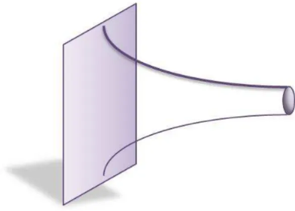
Figure 2.1: Multiple D1-branes (M2-branes) sticked in a D3-brane (M5-brane). In D3 point of view, this is a spike solution. On the other hand, we can see fuzzy S²solution in D1 point of view.

of D3-brane. If r is large, the direction of X⁹, a transverse direction to a D3-brane, goes to zero, but on the other hand if r goes to 0, X⁹ goes to infinity. This means this solution infinitely expands as an original D3-brane does, however if we close to its central region the solution lengthens to X⁹ direction. So this solution is called a spike solution. Note that there is a nice textbook to introduce the construction of this spike solution in Problem 20.6 and 20.7 of [42].

Let’s change our eyes to D1-branes picture. In D1-branes point of view, we consider the BPS equation of multiple D1-brane. We should consider Non-Abelian generalization of DBI action, but the expanded one around the flat spacetime. The action is same as the dimensional reduced action of 10-dimensional N = 1 super Yang-Mills action. The equations of motion are generally 2nd derivative equations and this can not be solved easily. So we concentrate on BPS equations which are 1st derivative equations. In the case for D1-branes we get [43]

∂Xⁱ

∂X⁹ ^∓ i 2^ϵ

ijk_[Xi_{, X}j_{] = 0} _(2.1.5)

where the indices i, j, k = 1, 2, 3 and X⁹ direction is one of D1-branes world coordinates. This equation is called Nahm equation. The solution of this equation can be obtained as [44]

Xⁱ =_± ¹ 2X⁹^σ

i_, _[σi_{, σ}j_{] = 2iϵ}ijk_σk_. _(2.1.6)

The matrices σⁱ obey SU (2) algebra above. This solution is a fuzzy S² solution which has SO(3) ≃ SU(2) global symmetry in non-commutative space. The fuzzy solution has a cutoff of its rank of irreducible representation. We choose the σⁱ to be in the N- dimensional irreducible representation of SU (2) with quadratic Casimir C = N² _{− 1, we} can describe a fuzzy S² radius as

R =

√(2πα^′)² N

∑

i

Tr(Xⁱ)² = ^2πα

′^√_N₂_{− 1}

2X⁹

−−−→ παN →∞ ^′ ^N

X⁹^. ^(2.1.7)

(12)

The solution we obtained in a D3-brane picture (2.1.4) has a continuum S². When we compare the D1-branes fuzzy solution to the continuum one, we should take the cutoff N → ∞. If we take the fuzzy sphere radius R as r, we see a perfect agreement (up to normalization) to the solution (2.1.4). This fact is an interesting consistency in string theory. Note that there is a brief review of D1-D3 system in [45].

So far we have reminded D1-D3 system in string theory, let’s turn to M2-M5 system in M-theory. We learned M2-branes and M5-branes really exist in M-theory, we should consider how to make M2-M5 system since it seems to exist also in M-theory in analogy with string theory. In D1 point of view in D1-D3 system, a commutator which includes in effective D1-branes theory is essential to obtain the fuzzy S² solution. However we need to construct a fuzzy S³ solution in M2-M5 system because of the difference of 3 space coordinates. Therefore we should take into account a triple algebra in this case. The expected BPS equation in M2-brane effective theory can be written as [45]

∂Xⁱ

∂s ⁺ λM₁₁³

8π ^ϵ

ijkl_[Xi_{, X}j_{, X}k_{] = 0} _(2.1.8)

where we use s as one of M2 world volume coordinates, M11 is Plank scale in 11D and λ is a arbitrary parameter. This BPS equation is called Basu-Harvey equation.

The solution of this Basu-Harvey equation is Xⁱ _∼ _√¹

s^G

i_, _[Gi_{, G}j_{, G}k_{] = ϵ}ijkl_GL _(2.1.9)

where we use generators Gⁱ which satisfy SO(4) algebra and have structure constants ϵ^ijkl. This algebra is called _A4 algebra. Reader may confuse to the usual SO(4) Lie algebra. However SO(4) construction in triple algebras can be obtained by using matrix representation. To realize a matrix representation, we need to reconstruct (or define) triple algebra to the form [G5, X^I, X^J, X^K] [46]. This fuzzy S³ solution (2.1.9) can be expanded to infinity as s→ 0 and can be regarded as single M5-brane.

2.1.3 Chern-Simons term

We have investigated about transverse scalars and their BPS solution. Let’s concentrate on gauge fields in multiple M2-branes. Gauge fields are important with respect to supersymmetric transformation. In D-branes case, we need gauge fields for closure of SUSY transformation. And also if we write DBI type of action as a D-brane effective action, gauge fields on a D-brane take a important role to understand the T-duality.

The effective action of multiple M2-branes action may have 8 transverse scalars X^I, 3- dimensional fermions Ψ and 1-form gauge field A_µ. First let’s count the d.o.f. of fermions [47]. There is 8 transverse direction, we need to keep maximally SO(8) R-symmetry. Only in 3-dimensional gamma matrices suggest us to have 2-component Majorana fermions, however we also have the other gamma matrices in transverse 8 directions. So we need to consider 10 gamma matrices and they make fermions to have 2⁵ components. When we consider about M2-branes we need to constraint ourselves to impose world parity on

(13)

2.2. REMARKABLE PROGRESS 1; BLG MODEL 9 M2-branes as Γ012Ψ = Ψ. This constraint is important for the closure of any symmetry in non-Abelian case (we will meet concrete examples of multiple M2-brane later, then you can see). Also equation of motion for fermions subtract the d.o.f. of fermions. Putting these all together, M2-brane fermions have 2⁵× 1/2 × 1/2 = 8 d.o.f.

To preserve SUSY, the d.o.f. of bosons should be equal to fermions. The transverse bosons are 8 and fermions are also 8. We might consider there are no need to introduce gauge fields in multiple M2-branes. However, as we will see, we really need gauge fields to close SUSY. How to realize zero d.o.f. of gauge fields ? We should introduce gauge fields as topological term. For the case for 3-dimension, we know very well it as Chern-Simons term.

∫

d³x tr [A∧ dA + A ∧ A ∧ A] . ^(2.1.10) Only with the Chern-Simons term, gauge fields propagate zero d.o.f. The necessity of Chern-Simons term is also important for conformal symmetry. When we have the kinetic term of gauge fields F², we cannot naively preserve conformal symmetry because its mass dimension is four.

We also comment in a case for D2-branes. For the fermions a situation is same as for M2-branes, so the fermions have 8 d.o.f. Since the transverse directions change to 7 for D2-brane, we only have 7 transverse scalars. There needs one more d.o.f. The lack of field can be compensate by introducing gauge fields. Gauge fields with usual kinetic terms F² essentially have d.o.f. of transverse direction only in world volume. So D2-brane gauge fields have one d.o.f. Putting it all together, we can show correct SUSY in D2-brane. This is different from M2-brane situation.

2 . 2 Remarkable progress 1; BLG model

There has been a remarkable progress in constructing N = 8 supersymmetric three- dimensional field theory with SO(8) R-symmetry by Bagger and Lambert and Gustavs- son. First Bagger and Lambert tried to construct multiple M2-branes effective action by using triple algebra, however they could not close SUSY algebra [1]. Afterward Bag- ger, Lambert [2] and also Gustavsson [3] introduced gauge fields and they succeeded to construct multiple M2-branes effective theory ¹.

2.2.1 Triple algebra

Bagger and Lambert introduced triple algebra and they investigated how to construct. To introduce triple algebra, we first define non-associative algebra.

< A, B, C >≡ (A · B) · C − A · (B · C). ^(2.2.1)

1Bagger and Lambert could construct the action, but Gustavsson wrote down only SUSY algebras. For this reason, the model sometimes has called BL model.

(14)

If product is usual, this non-associative algebra is zero. Using this non-associative algebra, we define triple algebra as

[A, B, C] =< A, B, C > + < B, C, A > + < C, A, B >

− < A, C, B > − < B, A, C > − < C, B, A > . ^(2.2.2) We can see the importance of non-associative algebra and its product to take triple algebra meaningful.

To take into account inner product, we also define the relation of trace. Trace operator should satisfy the relations.

tr(A, B) = tr(B, A), tr(A· B, C) = tr(A, B · C),

tr([A, B, C], D) =− tr(A, [B, C, D]). ^(2.2.3) This is a bilinear map; tr : A × A → C that is symmetric and invariant. These trace relation will be important to see invariance of gauge symmetry.

In this stage we write down the definition of structure constants of triple algebra and this can be considered also the definition of triple algebra.

[Tâ, T^b, T^c] = fâbcdTd. (2.2.4) With the last equation of (2.2.3), we can see the structure constant fâbcd should be completely anti-symmetric under exchange of indices.

We can consider gauge symmetry with triple algebra as

δX = Λab[T^a, T^b, X]. (2.2.5) This representation for gauge symmetry is correct since a variation of trace of same scalar fields is invariant under this transformation.

δ [tr(X, X)] = 2f^abcdΛ_abX_cX_d= 0. (2.2.6) Taking into account the gauge symmetry, we can introduce gauge fields and covariant derivative. The variation of gauge fields should be written as covariant derivative of gauge parameter.

δ ˜Aµ^b_a= ∂µΛ^˜^b_a_{− ˜Λ}^b_cA^˜µ^c_a+ ˜Aµ^b_cΛ^˜^c_a _{≡ D}µΛ^˜^b_a

A˜µ^ba≡ f^cdba^Aµcd, Λ^˜^b_a_{≡ f}^cdb_aΛcd (2.2.7) Then the covariant derivative can be read as

DµXa = ∂µXa_{− ˜}Aµ^b_aXb. (2.2.8) The gauge symmetry suggest important rule about structure constants. We need to consider “derivation” of triple algebra for gauge symmetry.

δ([X, Y, Z]) = [δX, Y, Z] + [X, δY Z] + [X, Y, δZ]. (2.2.9)

(15)

2.2. REMARKABLE PROGRESS 1; BLG MODEL 11 From this derivation we can get

[Tâ, T^b, [X, Y, Z]] =[[Tâ, T^b, X], Y, Z] + [X, [Tâ, T^b, Y ], Z] + [X, Y, [Tâ, T^b, Z]],

f^{ef g}_df^abc_g =f^{ef a}_gf^bcg_d+ f^{ef b}_gf^cag_b+ f^{ef c}_gf^abg_d. (2.2.10) This equation is called fundamental identity in triple algebra. In the case for commutator, we have Bianchi identity for Lie-algebra and (2.2.10) is considered as an triple algebra analogy of Bianchi identity. This fundamental identity is quite important to close SUSY algebras and construct examples.

2.2.2 Supersymmetry and BLG action

Bagger, Lambert and Gustavsson considered firstly to construct SUSY algebras in analogy with D2-branes effective action. They consider the main difference from D2-brane is to take into account triple algebra in stead of Lie algebra.

δX_a^I = i¯ϵΓ^IΨa

δΨa = DµX_aÎΓ^µΓÎϵ + κ[XÎ, X^J, X^K]aΓÎJKϵ

δ ˜A_µ^b_a = i¯ϵΓ_µΓ_IX_c^IΨ_df^cdb_a (2.2.11) where main difference exists at second term in the variation of fermion and κ is a arbitrary constant. In this transformation, we have 16 component of fermionic fields and supersymmetric parameter ϵ (they are constrained to preserve world sheet parity as Γ012ϵ =_−ϵ [1]).

For the closure of this SUSY algebra, we need to satisfy the relation; [δ1δ2]X_aÎ = v^µ(DµXÎ)a+ ˜Λ^b_aX_bÎ

[δ1δ2]Ψa = v^µ(DµΨ)a+ ˜Λ^b_aΨb

[δ1δ2] ˜Aµ^b_a = v^µF^˜µν^b_a+ (DµΛ)^˜ ^b_a (2.2.12) where we use bi-spinor vector v^µ and bi-spinor scalar ˜Λ^b_a defined as

v^µ _{≡ −2i¯ϵ}₂Γ^µϵ₁, Λ^˜^b_a _{≡ −i¯ϵ}₂Γ_JKϵ₁X_c^JX_d^Kf^cdb_a.

When we calculate left-hand sides of (2.2.12), we will meet extra terms of ¯ϵ2ΓµΓIJKL¯ϵ bi-spinor in the closure of Ψa and also ˜Aµ^b_a. For the closure of ˜Aµ^b_a, happily this term vanishes as a consequence of the fundamental identity (2.2.10). On the other hand for Ψa, these terms cancel if we choose the arbitrary constant

κ =₋¹

6^. ^(2.2.13)

(16)

The other redundant terms to obtain (2.2.12) can be regarded as on-shell condition or equations of motion. These can be read from (2.2.12) as

Γ^µDµΨa+¹ 2^f

cdb

a^Γ^IJ^Xc^I^Xd^J^Ψ^b ^{= 0,}

D²X_a^I₋ ⁱ 2^f

cdb

a^Ψ^¯^c^Γ^IJ^Xd^J^Ψ^b− ¹₂^f^bcda^f ef g

d^Xb^J^Xc^K^Xe^I^Xf^J^Xg^K ^{= 0,}

F˜µν^b_a+ ϵµνλf^cdb_a (

X_c^JD^λX_d^J + ⁱ 2^Ψ^¯^c^Γ

λ_Ψ d

)

= 0. (2.2.14)

The bosonic equations of (2.2.14) can be obtained by taking the supervariation of the fermion equation of motion.

To derive the equations of motion (2.2.14), we can guess an action as

L^BLG ⁼− ¹₂^tr(D^µ^X^I^{, D}^µ^X^I^{) +} ₂ⁱ^{tr( ¯}^{Ψ, Γ}^µ^D^µ^Ψ) + ⁱ

4^{tr( ¯}^{Ψ, Γ}^IJ^[X

I_{, X}J_{, Ψ])}

− ¹ 12^tr([X

I_{, X}J_{, X}K_{], [X}I_{, X}J_{, X}K_])

+ ¹ 2^ϵ

µνρ_(fabcd_A

µab∂νAλcd+² 3^f

cda

g^f^{ef gb}Â^µabÂ^νcdÂ^λef^). ^(2.2.15)

The potential term of scalar fields is sixth order as expected to be conformal because a mass dimension of scalar fields is 1/2 in three dimension. We can also see the existence of Chern-Simons term and the absence of gauge kinetic term F² as we have seen in section 2.1.3. This is surprising thing because we just order to keep supersymmetry. This action seems to preserve conformal symmetry even if quantized.

2.2.3 SO(4) BLG model

The BLG action (2.2.15) really has N = 8 as we saw, however there are some mystery to understand the triple algebras. One example can be easily obtained by setting the structure constant as

f^abcd = ϵ^abcd. (2.2.16)

Levi-Civita symbol with four-indices is only included in SO(4) algebra since it is invariant under SO(4) rotations. However unfortunately there are no-go theorem which shows SO(4) BLG is an only essential construction if we choose the group metric tr T^aT^b to be positive definite [48, 49].

The group SO(4) can be decomposed to SU (2) × SU(2). This decomposition can

(17)

2.2. REMARKABLE PROGRESS 1; BLG MODEL 13 really be done in SO(4) BLG model in [8]. The resultant action is

LSU (2)×SU (2) =_{− tr(D}^µX^I)^†DµX^I + i tr ¯Ψ^†Γ^µDµΨ + ^k

2π 1 2^ϵ

µνλ_tr

(

A^(L)_µ ∂_νA^(L)_λ +²ⁱ 3^A

(L) µ ^A^(L)ν ^A

(L) λ

)

− ^k 2π

1 2^ϵ

µνλ_tr

(

A^(R)_µ ∂_νA^(R)_λ + ²ⁱ 3^A

(R) µ ^A^(R)ν ^A

(R) λ

)

− ²ⁱ 3

2π k ^{tr ¯}^Ψ

†_Γ

IJ(XÎX^J†Ψ + X^JΨ^†XÎ+ ΨXÎ†X^J)

− ⁸ 3

( 2π k

)2

X^[IX^J†X^K]X^K†X^JX^I†. (2.2.17) The fields consist of two SU (2) gauge fields, having Chern-Simons terms with opposite levels. The Chern-Simons level k should be quantized and be integer because we need to have the action invariant under non-Abelian transformation of gauge group. All the matter fields transform as bi-fundamental of SU (2)_L_{× SU(2)}_R. In this representation, we have no more triple algebras but the well known SU (2) Lie algebras.

Let’s consider the moduli space of the action (2.2.17) by focusing on bosonic fields [50, 51]. Generic scalar configurations for which the potential vanishes correspond (up to gauge transformations) to diagonal matrices as

X^I = _√¹ 2

( z^I 0 0 z¯^I

)

. (2.2.18)

The gauge fields associated with the U (1) that rotates z^I and ¯z^I each other with the diagonal configuration (2.2.18). So we have

A^(L)_µ =

( a^(L)µ 0 0 _−a^(L)µ

)

, A^(R)_µ =

( a^(R)µ 0 0 _−a^(R)µ

)

(2.2.19)

with the normalization chosen to have gauge transformations

a^(L)_µ _{→ a}^(L)_µ _{− ∂}_µθ^(L), a^(R)_µ _{→ a}^(R)_µ _{− ∂}_µθ^(R). (2.2.20) where θ^(L,R) have period 2π.

The potential term is zero and the remaining kinetic term of the action changes to be S =

∫ d³x

[

−^∂^µ^z^I^{+ i(a}^(L)µ − a^(R)µ ^)z^I

2+ ^k 2π^ϵ

µνλ_(a(L) µ ^∂^ν^a

(L)

λ − a^(R)µ ^∂^ν^a (R) λ ⁾

]

(2.2.21) Then we combine the gauge fields linearly as

cµ = a^(L)_µ + a^(R)_µ , bµ= a^(L)_µ _{− a}^(R)_µ . (2.2.22)

(18)

By using this configuration the action rewritten as

LSU (2)×SU (2) =₋∂µz^I+ ibµz^I²+ ^k 4π^ϵ

µνλ_b µfνλ,

f_µν _{≡ ∂}_µc_ν _{− ∂}_νc_µ. (2.2.23) Since the new variable cµ of gauge field is usual U (1) gauge field and it should be satisfy Bianchi identity

ϵ^µνλ∂µfνλ = 0. (2.2.24)

To deal with the Bianchi identity together with the action, we take it as constraint term with Lagrange multiplier field σ(x).

Sconst.= ¹ 8π

∫

d³x σ(x)ϵ^µνλ∂µfνλ. (2.2.25) The Lagrange multiplier field σ(x) should be periodic because there is a monopole condition;

∫ d³x¹

2^ϵ

µνλ_∂

µfνλ =

∫

M

df =

∫

∂M

f _{∈ 4πZ.} (2.2.26)

Taking into this fact into account, the Lagrange multiplier field σ(x) should be periodic

σ(x)∼ σ(x) + 2πn ^(2.2.27)

where we use n as an integer. Together with this periodicity, the constraint term is harmless because e^iS^const = 1. This periodicity will be important to investigate the moduli space.

The equation of motion for f_µν determines bµ= ¹

2k^∂^µ^σ. ^(2.2.28)

Inserting the solution for bµ, the action becomes LSU (2)×SU (2)=₋

∂µz^I+ ⁱ 2k^z

I_∂ µσ

2

. (2.2.29)

In the final form of action (2.2.29), we have the gauge transformation

zÎ _{→ e}îα(x)zÎ, σ → σ − 2kα(x) ^(2.2.30)

We can now fix our gauge to set σ = 0. After doing this, we still have residual gauge transformation

α = ^πn

k ^(2.2.31)

(19)

2.2. REMARKABLE PROGRESS 1; BLG MODEL 15 which can be regarded as the periodicity for σ in (2.2.27). This residual symmetry give us a constraint for the scalar moduli should obey

z^I _{→ e}^πin^k z^I. (2.2.32)

There is also a discrete symmetry which changes a scalar moduli and its complex conjugate moduli as

z^I _{→ ¯z}^I. (2.2.33)

(2.2.32) tells us the moduli space should be divided by Z2k and (2.2.33) means to be divided by Z2. These orbifold projections do not commute with each other for k > 1, and the combined group is the dihedral group D2k. Finally we conclude that the moduli space for the level k in SO(4) BLG model is

(R⁸_{× R}⁸)/D2k. (2.2.34)

For the commute case k = 1, this is just

(R⁸ _{× R}⁸)/(Z2× Z2). (2.2.35) This analysis tells us that the SO(4) BLG model with Chern-Simons coefficient k is a effective theory of two M-branes living in orbifolded space.

In the supergravity picture, the orbifold moduli space R⁸/Z2k, except for k = 1.2, preserves as many as 12 supersymmetries orN = 6, and also gives rise to an R-symmetry SU (4)× U(1) [52, 53]. However, we have 16 supersymmetries in BLG model even when we turn on the integer coefficient k in front of the Chern-Simons term. This have still remained to be a mystery of BLG model.

F uzzy funnel solution and single M5

People might think the realization of Basu-Harvey equation and its classical solution which end on single M5-brane as we discussed section 2.1.2. The BPS equation of SO(4) BLG model is [54]

∂sX^A= mX^A+ ¹ 6^ϵ

ABCD_[XB_{, X}C_{, X}D_] _(2.2.36)

where we use s is one of world space coordinates of M2-branes and m is a mass. Since we can have rich structure of BPS solutions with mass term, first we turn on mass term and analyze BPS solutions.

The solution of the equation (2.2.36) can be obtained by using the solution which expand fuzzily

X^A=^{√ m} π

√ 1

1_{− e}^−2ms^T

A_, _[TA_{, T}B_{, T}C_{] = ϵ}ABCD_TD_. _(2.2.37)

(20)

If we wake s → ∞ the radius of solution becomes a constant and the solution goes to fuzzy S³ solution. On the other hand, if we take s→ 0 the radius goes to infinity and the solution with this limit represent single M5-brane. The hole shape of this solution looks like a funnel, so this solution is called fuzzy funnel solution. The shape have been already depicted as figure 2.1 (p.7).

Let’s evaluate the action with this BPS solution but without the mass. The fuzzy S³ radius can be estimated as

R² _≡ ^tr(X

A_{, X}A₎

nT2

(2.2.38) where n is a cutoff of irreducible representation, and T2 is tension of M2-brane. Then the action without time-integral which can be considered as energy density of this system is

E =

∫

d²x tr(∂sX^A, ∂sX^A⁾ _−−−→^n→∞ ^T

22

2π

∫ dx¹

∫

2π²R³dR

= T5

∫

d⁵x (2.2.39)

where in the first line we use BPS equation (2.2.36) on one-side and take the cutoff to diverge, and in the second line we use the explicit representation of tensions related as T5 = T₂²/2π. So we can conclude there exist BPS solution of multiple M2-brane which end on single M5-brane.

2.2.4 Lorentzian BLG model

There are no-go theorem which prevent us to construct the other model with positive metric in BLG model. SO(4) BLG model is just two M2-branes effective theory. If we would like to investigate more general multiple M2-branes, there need more than two. This is important when we deal multiple M2-brane effective theory with the dual supergravity language. So let’s change our eyes to allow a negative group metric. With a negative metric we can have the following structure by using the group generator T⁻¹, T⁰, Tⁱ [4–6].

[T⁻¹, T^a, T^b] = 0 [T⁰, Tⁱ, T^j] = f^ij_kT^k

[Tⁱ, T^j, T^k] = f^ijkT⁻¹ (2.2.40) where a, b run −1, 0, i and i, j, k run arbitrary. Using this algebras, we can know the metric of this system as

tr(T⁻¹, T⁻¹) = 0, tr(T⁻¹, T⁰) =_{−1, tr(T}⁻¹, Tⁱ) = 0, tr(T⁰, T⁰) = 0, tr(T⁰, Tⁱ) = 0,

tr(Tⁱ, T^j) = h^ij. (2.2.41)

We can see there is a negative metric. One can easily check that this triple algebra satisfies the fundamental identity (2.2.10). Since in (2.2.40) we only have the structure constants

(21)

2.2. REMARKABLE PROGRESS 1; BLG MODEL 17 as the usual Lie algebra, we have a possibility to describe multiple M2-branes. Since T⁻¹ commute all the other generators in the language of triple algebra, we can regard T⁻¹ as a center of the Lorentzian algebra (2.2.40).

Now we have the action with negative metric LL =

[

−¹ 2^{( ˆ}^D^µ^X^ˆ

I_{− B}

µX₀^I)²+¹ 4^(X

K

0 ⁾²^{([ ˆ}^X^I^{, ˆ}^X^J^])²− ¹ 2^(X

I

0^{[ ˆ}^X^I^{, ˆ}^X^J^])²

+ ⁱ 2^¯ˆΨΓ

µ_D_ˆ

µΨ + i ¯^ˆ Ψ0Γ^µBµΨ^ˆ ₋¹ 2^Ψ^¯⁰^X^ˆ

I_{[ ˆ}_XJ_{, Γ}

IJΨ] +^ˆ ¹ 2^¯ˆΨX

I

0^{[ ˆ}^X^J^{, Γ}^IJ^Ψ]^ˆ

+¹ 2^ϵ

µνλ_F_ˆ

µνBλ_{− ∂}µX₀^I BµX^ˆ^I ]

+_Lgh, L^gh ^{= (∂}^µ^X0^I^)(∂^µ^X−1^I ⁾− i ¯^Ψ⁻¹^Γ^µ^∂^µ^Ψ⁰ ^(2.2.42) where we have redefined the fields as

Xˆ _{≡ X}iTⁱ, Ψ^ˆ _{≡ Ψ}iTⁱ, A^ˆµ ≡ 2Aµ0iTⁱ, Bµ≡ Aµ ijf^ij_kT^k. The covariant derivative and the field strength

Dˆ_µ_{≡ ∂}_µX^ˆÎ+ i[ Â_µ, ˆXÎ], D^ˆ_µΨ_{≡ ∂}_µΨ + i[ ˆ^ˆ A_µ, ˆΨ], F^ˆ_µν = ∂_µA^ˆ_ν _{− ∂}_νA^ˆ_µ+ i[ Â_µ, Â_ν] (2.2.43) are the ordinary covariant derivative and field strength for the sub-algebra A. Since this action has a negative metric, we call this as Lorentzian BLG model. The specialties of Lorentzian BLG model are manifest SO(8) R-symmetry andN = 8, BF theory and usual Lie algebra [X, Y ]. There are ghost terms because of a negative metric. And we should consider whether this model is unitary and how to eliminate this ghost term or ghost degrees of freedom. With the negative metrics, there is also a no-go theorem [55]. So we have essentially SO(4) BLG model with positive metrics and Lorentzian BLG model with negative metrics.

The supersymmetry transformations for each mode are given by δX₀^I = i¯ϵΓ^IΨ0,

δX₋₁Î = i¯ϵΓÎΨ−1, δ ˆXÎ = i¯ϵΓÎΨ,^ˆ

δΨ0 = ∂µX₀^IΓ^µΓ^Iϵ,

δΨ−1 = _{∂_µX₋₁Î _{− tr(B}_µ, ˆXÎ)_}Γ^µΓÎϵ + ⁱ 6^{tr( ˆ}^X

I_{, [ ˆ}_XJ_{, ˆ}_XK_])ΓIJK_ϵ,

δ ˆΨ = D^ˆµX^ˆÎΓ^µΓÎϵ_{− B}µX₀ÎΓ^µΓÎϵ + ⁱ 2^X

0I^{[ ˆ}^X^J^{, ˆ}^X^K^]Γ^IJK^ϵ,

δ Âµ = i¯ϵΓµΓI(X₀ÎΨ^ˆ _{− ˆ}XÎΨ0),

δBµ = ¯ϵΓµΓI[ ˆX^I, ˆΨ]. (2.2.44)

The above construction of the 3-algebra contains the ordinary Lie algebra as a sub- algebra. The generators of the gauge transformation can be classified into 3 classes.

(22)

• I={T⁻¹⊗ T^a^{, a = 0, i}}

• A={T⁰⊗ Tⁱ}

• B={Tⁱ⊗ T^j}

Then it is easy to show that

[I, I] = [I, A] = [I, B] = 0, [A, A] = A, [A, B] = B, [B, B] = I ^(2.2.45) and hence the generators of A form a sub-algebra, which can be identified as the Lie algebra of N D2-branes. We will see concretely this gauge symmetry in section 3.2.

In Lorentzian action, we have another symmetry. The scaling of structure constants can be absorbed in redefinition of T⁰, T⁻¹ as we can see in (2.2.40). This means that the scaling of overall coefficient of the Lagrangian is a symmetry. To make this symmetry explicitely, we define a scaling of overall coefficient as 1/g². Then the theory has the symmetry

XˆÎ _{→ g ˆ}XÎ, X₀Î _→ ¹ g^X

I

0^, ^X⁻¹ → g³^X−1^I ^,

Ψˆ _{→ g ˆ}Ψ, Ψ0 _→

1

g^Ψ⁰^, ^Ψ⁻¹ ^{→ g}

3_Ψ

−1,

Aˆµ _{→ ˆ}Aµ, Bµ_{→ g}²Bµ. (2.2.46)

So the overall coefficient of Lorentzian BLG model is irrelevant. This Lagrangian has no free parameter. The original BLG action (2.2.15) can have the integer coupling in front of Chern-Simons term as essentially same way as (2.2.17). If we scale the matter fields as

X^I _→^{( k} 2π

)¹2

X^I, Ψ_→^{( k} 2π

)¹2

Ψ, (2.2.47)

then we obtain the action with overall coefficients k/2π. This overall coefficient takes a important role in CS theory, but is irrelevant in BF theory.

When we focus on the fields related to T⁻¹generator, we can see such kind of fields only included linearly. Therefore we can regard these fields X−1, Ψ−1 as Lagrange multiplier to obtain constraint equations

∂²X₀^I = 0, Γ^µ∂µΨ0 = 0. (2.2.48) If we consider these constraint equations and regard solutions of these constraint equations as effective couplings of Lorentzian BLG action, then we can treat the Lorentzian BLG model as a ghost-free action. This idea is important when we deal with conformal symmetry and compare with a result from the dual gravity picture (we will see explicitly in chapter 4, p.45).

(23)

2.2. REMARKABLE PROGRESS 1; BLG MODEL 19 D2 reduction

If the BLG model represents effective action of multiple M2-branes correctly, we can reduce the action to the effective action of multiple D2-branes. This can be done by taking a constant vacuum expectation value of scalar fields as

X₀^I = vδ^I,8, Ψ0 = 0. (2.2.49) This selection of the solution in the constraint equation (2.2.48) is compatible with the SUSY transformation and also the gauge transformation. The idea of giving a constant vev in the context of multiple M2-branes is firstly introduced by [56] in SO(4) BLG and [6] in Lorentzian BLG.

Taking this vev back to the Lorentzian action (2.2.42), then we obtain L = Tr

[

− ¹ 4v²^F^ˆ

2 µν− ¹

2^{( ˆ}^D^µ^X^ˆ

A₎2₊ ¹

4^v

2_{[ ˆ}_XA_{, ˆ}_XB_]2

+ⁱ 2^¯ˆΨΓ

µ_D_ˆ

µΨ +^ˆ ¹ 2^v^{¯ˆΨ[ ˆ}^X

A_{, Γ} 8,AΨ]^ˆ

]

. (2.2.50)

This is exactly the same action of multiple D2-branes and breaks conformal symmetry by giving a vev.

Ghost problem

There is a discussion to avoid ghost problem [57, 58]. Basic idea is to be gauged a constant shift symmetry of X₋₁^I , Ψ−1.

At casual glance at (2.2.42), we can see a constant shift symmetry;

δshX₋₁Î = ΛÎ, δsh = η. (2.2.51) If we impose this shift symmetry to be locally gauged, we need to add a new fields C_µÎ, χ as

Lnew=_−C_µ^I∂^µX₀^I+ ¯Ψ0χ. (2.2.52) When the new fields transform under gauged shift symmetry as

δshC_µ^I = ∂µδ^I(x), δshχ = iΓ^µ∂µη(x), (2.2.53) we can take the Lorentzian BLG action (2.2.42) with (2.2.52) to be invariant. Note that there is another new local symmetry defined as

δgC_µÎ = ∂^νΛ^¯_µνÎ , Λ^¯Î_νµ =_−¯ΛÎ_µν (2.2.54) Under this symmetry the new term (2.2.52) itself invariant.