本文 Thesis 総合研究大学院大学学術情報リポジトリ A1659本文

(1)

Distance and Proper Motion Measurement of The Red

Supergiant, PZ Cas, in Very Long Baseline

Interferometry H ₂ O Maser Astrometry

A Ph.D. Dissertation Presented to

Department of Space and Astronomical Science,

Graduate School of Physical Science,

The Graduate University for Advanced Studies

by

Kozue Kusuno

July 30, 2014

(2)

(3)

Abstract

Understanding mechanisms generation and preservation of spiral structure of spiral galaxies is an important theme in galaxy dynamics. Density wave hypothesis has been considered to play a major role to form spiral arms in the Milky Way. One of predicts of the hypothesis is that young objects on the spiral arms should have peculiar motions no larger than 10 km s⁻¹, which align each other in the outer Galaxy. On the other hand, VLBI astrometric observations have recently detected randomly directed peculiar motions of 20–30 km s⁻¹ in number of high-mass star-forming regions. This thesis study has been conducted to understand the origin of large peculiar motions on the spiral arms in the Milky Way. We performed VLBI H2O maser monitoring observations of the red supergiant, PZ Cas, at twelve epochs from 2006 April to 2008 May using VLBI Explo- ration Radio Astrometry (VERA). We fitted maser motions by a simple model composed of a common annual parallax and linear motions of the individual masers. The parallax subtracted maser motions were well modeled by combination of a common stellar proper motion and a radial expansion motion of the circumstellar envelope. We obtained the annual parallax of 0.356 ± 0.026 mas and the stellar proper motion of µ^∗^αcos δ = −3.7 ± 0.2, and µ^∗δ = −2.0 ± 0.3 mas yr⁻¹ eastward and northward, respectively. The annual parallax corresponds to a trigonometric parallax of 2.81^+0.22_−0.19 kpc. By re-scaling the luminosity of PZ Cas in any previous studies using our trigonometric parallax, we locate PZ Cas on a H-R diagram and found that it approaches towards a theoretically evolutionary track of an initial mass of ∼ 25 M^⊙. The sky position and the distance to PZ Cas are consistent with the OB association, Cas OB5, which is located in a molecular gas supershell. We derived the peculiar motion of PZ Cas of Us = 22.8 ± 4.4, V^s = 7.1 ± 2.2, and Ws = −5.7 ± 4.0 km s⁻¹. We discussed three possibilities to explain the peculiar motion. We firstly compared the peculiar motions of PZ Cas and Cas OB5 to examine a runaway star hypothesis. Because PZ Cas’s peculiar motion is close to the median of the distribution of the Cas OB5 member stars, we concluded that PZ Cas has a typical motion of Cas OB5. On the contrary, this means that Cas OB5 has a large peculiar motion. We secondly compared the peculiar motions of Cas OB5 with Cas OB4. Because Cas OB5 is located at the western edge of an HII supershell while the Cas OB4 is located at the eastern side, an expanding motion in those OB associations was expected to be observed, although the velocity dispersions of the OB associations are very large. The problem with this hypothesis is that there are not enough energy sources to form the supershell so far. The last possibility is epicyclic motion hypothesis in galaxy dynamics. Recent large

(4)

formed in a disk galaxy without the density wave. According to the simulation results, young objects in the disk have a randomly large peculiar motions because of the epicyclic motions as large as what the VLBI astrometric observations have shown. At this moment, although we have no concrete evidence to conclude which hypotheses between the later two explain the origin of the peculiar motion of PZ Cas, the epicyclic motion hypothesis may be plausible because of the lack of the energy source to form the supershell.

(5)

List of Figures

2.1 Cas OB5 member stars . . . 21

2.2 Conceptual illustration of the VERA . . . 22

2.3 Steward-mount dual-beam platform of the VERA antennas . . . 23

2.4 Time variation of system noise temperature at epoch F . . . 24

2.5 Block diagram of the Direct Phaser Transfer . . . 25

2.6 Complex gain calibration solutions obtained from J2339+6010 at epoch F for the phase referencing . . . 26

2.7 Block diagram of the ordinary AIPS phase referencing analysis to generate an AIPS CL table . . . 27

2.8 Phase calibration data as shown in Figure 2.5 . . . 28

2.9 Phase solutions using the fringe-fitting with the solution interval of 20 min for the PZ Cas’s brightest velocity channel at epoch F . . . 29

2.10 Astrometric observation simulation results for the pair of PZ Cas and J2339+6010 . . . 30

2.11 Spatial distribution of the PZ Cas H2O masers . . . 31

2.12 Spatial motions of 10 isolated maser spots . . . 32

2.13 Spatial motions of blended maser spots . . . 33

2.14 Least-square fitting results of the motions of the maser spot . . . 34

2.15 Histograms of individual annual parallaxes for 16 maser spots . . . 35

2.16 Position residuals of the 16 maser spots after removing the annual parallax of 0.356 mas, proper motions, and initial positions . . . 36

2.17 Internal motions of maser spots around PZ Cas . . . 37

3.1 Locations of PZ Cas on the H-R diagram . . . 53

3.2 The peculiar motion of U and V components of PZ Cas and other maser sources on the Galactic plane . . . 54

3.3 Peculiar motions of the sources in each of Perseus arm and Local arm . . . 55

3.4 Proper motions of the Cas OB5, Cas OB4, and Cas OB7 members . . . 56

3.5 Histogram of each of the three components of the peculiar motion of the fourteen sources in Cas OB5 . . . 57

iii

(8)

3.6 Histogram of each of the three components of the peculiar motion of the twelve sources in Cas OB5 . . . 58 3.7 Three dimensional views of positions and peculiar motions of the member

stars of Cas OB5, Cas OB4, and Cas OB7 . . . 59 3.8 Peculiar motion of the member stars of Cas OB5 and Cas OB4 . . . 60

(9)

List of Tables

2.1 Observing epochs of PZ Cas astrometric monitoring observations . . . 38

2.2 Frequency allocation for PZ Cas and J2339+6010 at epoch F . . . 39

2.3 Phase tracking center positions of the observed sources . . . 40

2.4 Annual parallax results of PZ Cas . . . 41

2.5 Proper motions, initial positions, and parallaxes of the PZ Cas H2O maser spots . . . 42

2.6 Proper motions and initial positions of the maser spots detected at least in two epochs . . . 43

2.7 Astrometry analysis results of PZ Cas . . . 44

3.1 Proper motions of the member stars of Cas OB5 . . . 61

3.2 Proper motions of the member stars of Cas OB4 and Cas OB7 . . . 62

A.1 H2O maser spots table of PZ Cas at epoch A . . . 74

A.2 H2O maser spots table of PZ Cas at epoch B . . . 75

A.3 H2O maser spots table of PZ Cas at epoch C . . . 76

A.4 H2O maser spots table of PZ Cas at epoch D . . . 77

A.5 H2O maser spots table of PZ Cas at epoch E . . . 78

A.6 H2O maser spots table of PZ Cas at epoch F . . . 79

A.7 H2O maser spots table of PZ Cas at epoch G . . . 80

A.8 H2O maser spots table of PZ Cas at epoch H . . . 81

A.9 H2O maser spots table of PZ Cas at epoch I . . . 82

A.10 H2O maser spots table of PZ Cas at epoch J . . . 83

A.11 H2O maser spots table of PZ Cas at epoch K . . . 84

A.12 H2O maser spots table of PZ Cas at epoch L . . . 85

v

(10)

(11)

Chapter 1 Introduction

1.1 Spiral Structure of the Milky Way

The Milky Way is one of important astronomical objects gathering more than 200 billion stars in the convex, which rotates with an independent rotational speed of ∼220 km s⁻¹ (Kerr & Lynden-Bell 1986). The diameter of the Milky Way is about 30 kpc, and the total mass is about 10¹¹ M⊙. The Milky Way is thought to be a typical spiral galaxy which consists of a central bulge with a bar structure, and multiple spiral arms. The spiral structure of the Milky Way was first recognized by Georgelin & Georgelin (1976) who measured kinematic distances of Galactic HII regions in the whole Milky Way. It is divided into three classes: disk bright stars with ionized hydrogen region born in spiral arms, brightest and dense bulge stars, and halo with globular clusters. In addition to the stellar objects, interstellar medium composed of gas and dust exist with the mass of 1/20 and 1/2000 in the total mass of the stellar object in the Milky Way, respectively. The interstellar medium is distributed in the thin disk extendedly similarly with the distribution of the stellar object. One of major subjects of spiral galaxies is how they maintain their spiral structures. It is a wellknown phenomenon that spiral galaxies have flat rotation curves in which the rotation velocity does not depend on the Galactocentric distance, so that the spiral galaxies show a differential rotation. If the spiral structure comes from the rotation of the materials, it cannot be maintained for longer than several rotation periods, because the closer the material is located to the center the shorter the one revolution. This leads to a so-called winding problem.

A “density wave theory“ was proposed as a hypothesis to solve the winding problem by C. C. Lin and F. Shu in 1964. According to the hypothesis, the spiral structure is considered to be a result of propagation of a stationary density enhancement pattern (density wave) through a galactic disk with restorative forces stimulated by swing amplification (Toomre 1981, in Structure and Evolution of Normal Galaxies, ed. S. M. Fall

& D. Lynden-Bell, 111-136). The interstellar medium orbiting in the disk is compressed 1

(12)

by a shock front when the density wave passes through. In a spiral galaxy, arms are composed of giant molecular clouds (GMCs) and more massive objects (giant molecular associations: GMAs), and young stars born in such clouds which are trailing the increased density of the materials. The density wave hypothesis predicts that there is a corotation radius at which an angular velocity of the density wave is equal to that of the galactic rotation. For example, it is considered that the density wave rotates at an angular velocity of roughly half of the galaxy rotation speed in the solar neighborhood. When the rotating materials pass the density wave, perturbation and shock are induced in the interstellar materials. Gases are compressed to increase the density to a factor of 5–8 higher than before in the vicinity of the spiral arms, and the maximum peaks of the density are often observed as dark lanes along the spiral arm. The gas compression along the spiral arms makes a trigger of gravitational instabilities to form stars. One of the characteristics of the density wave hypothesis in the galaxy dynamics is that young objects tend to deviate from the galactic rotation because a shear of the shock front induced by the density wave are formed in the spiral arms. We refer such an extra motion from the galactic rotation as to a “peculiar motion” or “non-circular motion”. It is considered that the peculiar motions are not randomly directed but aligned well each other with a typical speed less than 10 km s⁻¹.

In terms of the Milky Way, the number of spiral arms and entrainment degree has not been understood well (Russeil 2003) because it cannot be possible to measure the Galactic objects in the disk accurately enough to discuss, especially for regions beyond the Galactic center.

1.2 Astrometry of Galactic Object

There are three methods to measure distances to Galactic objects. The first method is the photometric parallax for stellar clusters. From a Hertzsprung-Russell diagram (H-R diagram) of star cluster, the class, the spectral type, and the absolute magnitude of the stars is associated. In comparison with the spectra of the cluster observed accurately on the H-R diagram, we can calculate the absolute magnitude. Therefore, we evaluate a distance modulus of the main sequence as well as interstellar extinction. Because of a difficulty in evaluating the degree of the extinction, the photometric parallax has typically 20–30% uncertainty (Menten et al. 2007; Zhang et al. 2012b).

The second is the kinematic distance method, which has been used for estimating the distances to Galactic GMCs. By measuring radial velocities of the clouds, we can retrieve the distances with an assumption of the Galactic rotation curve. The measured distances by this method tend to be larger, sometimes by factors greater than 2, than the annual parallax (Reid et al. 2009b).

(13)

1.3. RED SUPERGIANT STARS 3 The last one is the annual parallax method to measure a tiny positional modulation caused by the Earth’s orbital motion in a year. We are measuring the annual parallax of the sources with strong maser emission associated with high-mass star-forming regions (HMSFRs) and red supergiants, using Very Long Baseline Interferometry (VLBI) techniques. This method can determine source distances directly and geometrically without any assumptions of luminosity, extinction, metallicity, crowding, and so on. In addition, proper motions of sources can be obtained as well by monitoring the positional changes. Hipparcos project made great successes in measuring annual parallaxes of stars distances less than several hundred parsecs with an accuracy of 1 mas (Battrick 1989). Information of trigonometric parallaxes and proper motions together with radial velocities enable us to investigate three dimensional (3-D) motions of the stars in the Milky Way. VLBI astrometry is a very powerful tool to measure annual parallaxes of Galactic maser sources farther than sub-parsec distance: 52 maser sources have been measured using the Very Long Baseline Array (VLBA), VLBI Exploration of Radio Astronomy (VERA), and the European VLBI Network (EVN) (Reid et al. 2009b; Honma et al. 2012). A typical measurement accuracy of the distance of phase referencing VLBI observations is about 10 % (Ando et al. 2011; Asaki et al. 2010; Bartkiewicz et al. 2008).

1.3 Red Supergiant Stars

Red supergiants (RSGs) are evolved from massive OB stars (10M^⊙ _{≤ M ≤50M}^⊙) after they leave a main-sequence in the H-R diagram (e.g. Massey 2003). They eventually become Wolf-Rayet stars phase and/or supernovae. RSGs are in He-burning phase of the massive stars. Their spectral types are K or M, and effective temperature is 3500−4500 K (Massey 2003). Radii of massive stars increase to 300−2000 R^⊙ in the RSG phase, and thus the luminosities reach 10⁴_–5×10⁵ L^⊙. Although RSGs are very important to understand the last stage of the evolution of massive stars, it is observationally difficult to study RSGs because the number of massive stars is much smaller than that of low- mass stars in the Milky Way, and because the RSG phase is too short. For instance, the population of observed RSGs in the Milky Way is less than 100 among the total number of the stars of 200 billions, and very short duration of the RSG phase of typically ∼ 10² ^yr makes it difficult to observe them. Circumstellar envelopes (CSEs) expanding outward from a central RSG as a stellar wind are often observed. Mass-loss rates of RSGs ranges 10⁻⁷–10⁻⁴ M^⊙ yr⁻¹. Since envelopes often obscure the central stars, we have difficulties to obtain precise physical parameters of the central stars.

Bright masers are observed in CSEs of the RSGs at radio frequencies (e.g. Choi et al. 2008; Asaki et al. 2010). Because an intrinsic size of a maser source is typically 1 AU (Elitzur 1992), maser sources farther than a few kpc can be treated as point-like

(14)

sources in the VLBI observations. Using phase referencing VLBI techniques, we can measure tiny spatial motions of the masers which compose of internal motions because of CSE’s expansion, annual parallaxes, and systemic proper motions of central stars. Precise annual parallax measurements provide us absolute magnitude of stars. In the RSG phase, a location in the H-R diagram is not strongly dependent on the effective temperature. By comparing the absolute magnitude with evolutionary tracks for various initial mass of massive stars, the initial mass of the star can be derived (Choi et al. 2008). Recent observational studies with the MERLIN suggest that H2O masers around RSGs may be stable for longer than several years (Richards et al. 2012) while those masers of low- and intermediate-mass evolved stars can survive only for a few months. Therefore, the H2O maser emissions of RSGs is considered to be a good probe to trace the CSEs in a long-term VLBI monitoring program.

RSGs are often observed in large star clusters in which more than several OB stars and RSGs are included. Such a star cluster is called an OB association whose typical size is ∼ 200 pc. OB associations are located around GMCs or H^II regions, and form parts of large-scale star-forming regions. The typical age of OB associations is about 10⁶–10⁷ yr, and the mass is about 10³–10⁴ M⊙. Member stars of the OB associations were firstly catalogued by Humphreys (1978), and was later updated by Garmany & Stencel (1992). Asaki et al. (2010) obtained the 3-D motion of another RSG, S Per, and found its systemic peculiar motion of 15 km s⁻¹. Considering the age of S Per being a few tens of million year, it is unlikely that the star shows a large peculiar motion which old stars often have. Asaki et al. (2010) pointed out that, since S Per is involved in the Per OB1 association, such a large peculiar motion of the RSG may be related to the whole motion of the Per OB1 association in the Milky Way. It is quite important to know whether RSGs’ motions are aligned with their accompanying OB associations or not for further discussions about the Milky Way dynamics. In addition, RSGs can become distance indicators for OB associations by measuring the annual parallaxes very precisely with phase referencing VLBI. To determine trigonometric distance to OB associations is important for verification of the calibration method of the distance ladder.

1.4 Astronomical Masers

1.4.1 Maser Physics

Astronomical masers were firstly reported by Weaver et al. (1965) and Gundermann (1965) as intense OH radiations from several Galactic HII regions in their 18 cm wavelength observations. Those intense radiations were explained by Perkins et al. (1966) and Litvak et al. (1966) using a theoretical idea of amplification caused by inverted populations be-

(15)

1.4. ASTRONOMICAL MASERS 5 tween energy states of OH molecules. Intensive emission from materials with the inverted populations is referred to as Microwave Amplification by Stimulated Emission of Radia- tion (maser). In the regions radiating astronomical masers, the population on the energy states of maser molecules do not follow the Boltzmann distribution. The population of specific two energy states does not form the thermal equilibrium, so that the number of molecules at the higher energy state is larger than that at the lower state.

The population inversion is caused by enhanced excitation to a higher energy state by kinematical interactions in gas clouds (collisional pumping) or irradiation of strong infrared flux (radiative pumping). Let us introduce the standard radiative transfer equation,

dIν

dl ^{= −κI}^ν ^{+ ǫ} ^(1.1)

to develop a theoretical explanation of the maser emission. Here Iν is a radiation intensity, l is a path length in the medium that the light is passing through, κ is a volume absorption coefficient, and ǫ is a volume emission coefficient. Here κ and ǫ is given by

κ = ^hν

4π∆ν⁽ⁿ¹^{− n}²^)B, ^(1.2)

ǫ= ^hν

4π∆νⁿ²^A, ^(1.3)

where n1 and n2 are a population densities of the lower and upper energy state of the molecules, A and B are a Einstein coefficients for spontaneous and stimulated emission respectively, h is Planck’s constant (= 6.63 × 10⁻³⁴ Js), ν is a center frequency of the line spectrum, ∆ν is a Doppler line width. Assuming that κ and ǫ are constant in the medium, equation (1.1) is solved as follows:

I(l) = I(0)exp(−τ) + ^κ_ǫ{1 − exp(−τ)}, ^(1.4) Here, the Rayleigh-Jeans approximation can be used in the microwave region as follows:

TB = ^c

2

2kBν²^I, ^(1.5)

where TBis brightness temperature, and kBis Boltzmann’s constant= 1.38×10⁻²³^{J K}⁻¹^. Then, we can express equation (1.4) using the brightness temperature:

TB _{= [T}B_{(0) − T}_x]exp(−κl) + T^x^, ^(1.6) where Tx is excitation temperature for the transition. In the thermal equilibrium, Tx can be defined by

n₂ n1

= exp (

−_k^hν

BTx

)

. (1.7)

(16)

If there are too many molecules in the upper energy state, we have the population inversion as n2 > n1 in equation (1.7). This leads to κ < 0 in equation (1.2). In this case, an optical depth (τ ) takes a negative value, so that exponential amplification is caused rather than a decrease of the intensity as radiation travels along the pass. We have to note that the excitation temperature also becomes negative in the population inversion. Thus, as long as the population inversion persists, and as long as the region which contribute to maser photons with equally the radial velocity and the Doppler frequency continued, the maser emission is amplified.

Maser emission has been found from OH, H2O, SiO, NH3, and CH3OH molecules. The astronomical maser emission has been observed from comets, molecular clouds in star- forming regions, CSEs of evolved stars, and active galactic nuclei. Very intensive masers are often observed in star-forming regions and evolved stars in the Milky Way. Therefore, the maser is one of the very important probes to study stars in the phases of their birth and death. The maser is also used to study scattering of the Galactic interstellar medium or to measure annual parallaxes of distant Galactic objects because angular size of the maser emitting region is very compact to be resolved as point source.

1.4.2 Stellar Masers

Stellar masers are often observed from red giant stars or red supergiant stars. Hereafter, we refer to those objects as evolved stars. Strong stellar masers are specially found from long period variable (LPV) stars with strong infrared excesses. These stars are surrounded by thick CSEs of gas and dust. Therefore, the stellar masers are related to the mass ejection from a central star.

Four molecules are known to emit astronomical masers from evolved stars in the radio wavelengths: SiO, H2O, OH and HCN. Input energy to excite maser emission is 1800, 600, and 0 K for SiO (v = 1), H2O, and OH molecules, respectively. SiO masers are excited at the vicinity of the central star (R∗ _{∼ 10}²_{− 10}³ R⊙). The H2O maser sources are located in the CSE just outside the SiO maser region (≤ 10⁴ ^R^⊙), and the OH masers are located at the outermost part of the CSE (> 10⁵ R⊙).

We here describe the H2O stellar masers in the evolved stars in more detail. Typical isotropic photon luminosities of LPV stars are about ∼ 10⁴ ^L^⊙, while RSGs emit around

∼ 10⁵ ^L^⊙. However infrared radiation from the central stars cannot excite the water molecules required for the observed water maser brightness. A velocity profile of the H2O masers show time variation in a time scale from a few weeks to a few months. Although a time variation of stellar masers shows a good correlation with the stellar luminosity cycle, the H2O maser maximum have a time phase lag of 0.1–0.2 period from the infrared and OH maser time variations (Engels et al. 1986). Therefore, the excitation mechanism of the stellar H2O masers is considered to be the collision pumping (Deguchi 1977) rather

(17)

1.5. ASTROMETRY WITH VLBI PHASE REFERENCING TECHNIQUES 7 than the radiative pumping.

1.5 Astrometry with VLBI Phase Referencing Tech-

niques

Several kinds of techniques have been developed for the VLBI astrometry to obtain ac- curate positions of compact radio sources. The most successful techniques is phase referencing, in which a target source is observed almost simultaneously with closely located reference sources. By subtracting fringe phases of a reference source from target fringe phases, a large amount of VLBI interferometer phase errors due to uncertainties in fluc- tuating atmosphere, frequency and clock standards, Earth orientation parameters, and baseline vectors between VLBI stations can be eliminated (Asaki et al. 2007). The first successful experiment of VLBI phase referencing was demonstrated by Bartel et al. (1986) for a pair of quasars, 3C345 and NRAO512. They showed that relativistic jet components of 3C345 are moving with subluminal speeds while the radio core is positionally very stable. Recently, Hada et al. (2011) investigated the radio core positions of M87 at the various frequencies with the VLBA using the phase referencing to determine the super massive black hole position. They observed the core of the AGN jet in several frequencies by using the phase referencing technique. They found that the central engine of M87 is located within 14–23 Schwarzschild radii of the radio core at 43 GHz.

Astrometry of Galactic maser sources is an important scientific target to study kine- matics of the HMSFRs and evolved stars as well as the galaxy dynamics by measuring the positions of the stars in the sky with respect to a distant quasars as a positional reference. Xu et al. (2006) measured the distance to the W3(OH) HMSFRs in the Perseus arm using the VLBA. They observed for 8 hours on each of five epochs in 2003–2004. The distance to W3(OH) was successfully determined to be 1.95 ± 0.04 kpc. The photometric distance of W3(OH) is ∼2.2 kpc, so that they updated the distance with an accuracy of ∼ 2%. A number of astrometric observations with the H2O masers at 22 GHz and methanol masers at 12 GHz have been carried out using the VLBA (Sanna et al. 2009; Reid et al. 2009a; Moscadelli et al. 2009; Xu et al. 2009; Zhang et al. 2009; Brunthaler et al. 2009). On the other hand, the VERA has observed the H2O maser and SiO masers at 43 GHz towards HMSFRs and evolved stars (Asaki et al. 2014; Hirota et al. 2007; Choi et al. 2008; Sato et al. 2008).

(18)

1.6 Dissertation Goals

VLBI astrometry has revealed distances and 3-D motions of a number of Galactic maser sources in the last several years. Very precise astrometry with the VLBI techniques has just opened a new era for the Milky Way research with a typical accuracy of a few tens of micro arcseconds. Now we are able to pursue several spiral arms in the Milky Way with HMSFRs and RSGs close to the Sun (Reid & Honma 2013). The accumlation of the kinematic information of the Galactic objects will cover many research fields in astronomy and astrophysics including kinematic research of maser spots of star forming regions and stars, and in a quest of dynamical structure of the Milky Way to obtain fundamental parameters such as the distance from the Sun to the Galactic center, the rotation curve, and the solar motion.

On the other hand, we are also facing new questions in this research field. One of them now confusing us is large peculiar motions of HMSFRs. If the spiral structure of the Milky Way is formed by the propagation of the density wave, the young objects would not have large peculiar motions; the reality is that many of the sources have peculiar motions of 10–30 km s⁻¹. Although the origin of such large peculiar motions can be sometimes explained in line of super bubble due to supernova explosions (Sato et al. 2008) or cloud shuffling (Lee & Lim 2008), we cannot always find concrete reasons to cause such large peculiar motions.

To improve our understanding about the large peculiar motions in the Milky Way, we have investigated the 3-D motion of one of the RSGs, PZ Cas. In this study we selected this source with the following reasons:

(1) H2O masers in the CSE of this star are stably observed for longer than a few years, the annual parallax and systemic proper motion of the central star can be estimated with high accuracy and reliability;

(2) The star is involved in a OB association, Cas OB5, which is considered to be located in the Perseus spiral arm (Humphreys 1978). Thus PZ Cas is probably located in the Perseus arm; and

(3) The star is as young as a few to a few tens of M yr so that the peculiar motion of this target has not been gravitationally affected by other Galactic objects. PZ Cas and the member stars of Cas OB5 are located at the western edge of a HI

supershell (Fich 1986), hence we can investigate whether the expanding motion of the shell affect the peculiar motion(s) of the stars.

In this thesis, we aim to achieve the following subjects to tackle the most important science theme; to search for the origin of the large peculiar motions of young objects in the spiral arms.

(19)

1.6. DISSERTATION GOALS 9 (1) we make the H2O maser image of PZ Cas for the first time.

(2) In order to track the maser emissions as long as possible, we improve the data reduction scheme to compensate the lack of the sensitivity.

(3) We measure the annual parallax and systemic proper motion of the central star very precisely to obtain the peculiar motion of the star.

(4) Using the obtained distance, the astrophysical parameters of PZ Cas such as the luminosity and the initial mass are updated.

(5) We investigate whether the peculiar motion of PZ Cas is comparable to those of the other Galactic sources in the Perseus spiral arm. If it is as large as those of the other sources, we pursuit the origin of the peculiar motion.

For the above purposes, we made use of the VERA archive data of PZ Cas monitoring program conducted from 2006 Apr to 2008 May, almost two years, with VLBI phase referencing technique. In Chapter 2, observation and data reduction of PZ Cas are described. Results of the monitor program are shown in Chapter 2 as well. We discuss the research results in Chapter 3. We summarize our conclusions in Chapter 4.

(20)

(21)

Chapter 2 VLBI Astrometry Observations of

Red Supergiant

In Chapter 2, first we describe characteristics of the target source, PZ Cas, and its environment. Next we mention the VLBI phase referencing observations for the source using the VERA. Several aspects of the VLBI array are also described. We introduce a new phase correction method called Direct Phase Transfer in the part of the data reduction. Finally we figure out astrometric results for PZ Cas.

2.1 Observational Target and Environment

In this study, our main research target is VLBI astrometry for the red supergiant, PZ Cas. Spectrum type of PZ Cas varies in M2-M4Ia. According to General Catalogue of Variable Stars (GCVS), PZ Cas is a semiregular variable star with the period of 925 days. The minimum and maximum values of the magnitude is 11.6 and 12.9, respectively. The effective temperature of PZ Cas is calculated to be 3600 K (Levesque et al. 2005). Mass loss rate is computed to be 6.5 × 10⁻⁶ ^M^⊙ ^yr⁻¹ (Mauron & Josselin 2011).

H2O and OH masers have been detected in the spectrum profile of the star (Dickinson 1976; Dickinson & Chaisson 1973). On the other hand, SiO masers detection has not been reported yet. The H2O maser profiles of PZ Cas show double peaks (Dickinson 1976). Later its profile was changed to a single peak spectrum (Shintani et al. 2008). Spatial distribution of the H2O and OH masers around PZ Cas has not been imaged.

PZ Cas is catalogued as a member star of an OB assoaication, Cas OB5 (Humphreys 1978; Garmany & Stencel 1992). According to Garmany & Stencel (1992), the Cas OB5 association has 65 member stars including five RSGs as shown in Figure 2.1. Hipparcos (Perryman et al. 1997) has measured proper motions of 15 stars out of the 65 stars. The photometric parallax to Cas OB5 is reported to be 2.5 kpc (Humphreys 1978). Fich (1986) reported that there exists a large shell-like structure (supershell) to Cas OB5 with

11

(22)

the radius of 190 pc, the velocity of ∼ 20 km s⁻¹, and blown mass of ∼ 7.5 × 10⁵ ^M^⊙^.

2.2 VERA Observations of PZ Cas

The VERA is a Japanese VLBI array of National Astronomical Observatory of Japan (NAOJ) for conducting VLBI phase referencing astrometry observations. A conceptual illustration of the VERA is shown in Figure 2.2. The VERA has four antennas located at Mizusawa, Iriki, Ogasawara, and Ishigakijima (coded as MIZNAO20, IRIKI, OGASA20, and ISHI- GAKI, respectively) with baseline range from 1000 km to 2300 km. Each radio telescope has 20m aperture size in diameter. The main project of the VERA is to explore the 3-D structure and dynamical of the Milky Way based on high-precision astrometry of Galactic maser sources. A significant feature of the VERA antennas is the dual-beam receiving system as shown in Figure 2.3 which allows us to simultaneously observe a target and reference source within 2^◦.2 (Honma et al. 2003). Main observing frequency bands of the VERA are K-band (22 GHz) and Q-band (43 GHz). Annual parallaxes of 17 Galactic water maser sources have been measured using the VERA at 22 GHz (Honma et al. 2012). VERA of PZ Cas at 22.2 GHz have been conducted at 12 epochs over two years. The observing epochs are listed in Table 2.1. In our monitoring program, one beam (beam A) observed PZ Cas, and another (beam B) observed a closely located continuum source, J233921.1+601011 (hereafter, abbreviated as J2339+6010), one of the VERA 22 GHz calibrator survey sources (Petrov et al. 2007), 1.7^◦ away, as a position reference. The observation duration was eight to ten hours. Each observation was divided into several sessions for the simultaneous tracking of PZ Cas and J2339+6010, each separated by short-term sessions of bright calibrators (3C 454.3 and J230043.0+165514) for 15 min in order to check the observing systems. We prepared one baseband channel (BBC) with a bandwidth of 16 MHz for PZ Cas and 14 BBCs with a total band width of 224 MHz for J2339+6010 in left-hand circular polarization. VLBI cross correlation was carried out with the Mitaka FX correlator at NAOJ, Mitaka, Japan, to produce VLBI fringe data with 512 spectral channels for PZ Cas for the central 8 MHz bandwidth, corresponding to a velocity spacing of 0.2107 km s⁻¹ for the H2O J^K₋^K+ = 616_{− 5}23 maser line. A typical frequency allocation after the cross correlation is listed in Table 2.2.

2.3 Data reduction

To describe the phase referencing and imaging analysis process, we often refer results of a specific epoch observation (epoch F on Mar 22, 2007) because we started the data analysis with this epoch data. We analyzed the VLBI data using the standard NRAO data reduction software, Astronomical Image Processing Software (AIPS), version 31DEC10.

(23)

2.3. DATA REDUCTION 13

2.3.1 Initial calibrations

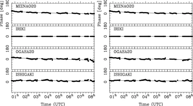
Initial calibration tasks were common for both PZ Cas and J2339+6010. First, the amplitude calibration was carried out by using the system noise temperatures (Tsys) and gain calibration data. The measurements of Tsys often have abrupt time variations, as shown in Figure 2.4, especially when rain falls happened during the observation. We consider such rapid and abrupt time variations owing to an absorption effect of water puddles on the top of the VERA antenna feedome. We carried out a polynomial fitting of the raw Tsys data after removing such abrupt changes. At epoch H, since Tsys was not recorded for either beams A or B of ISHIGAKI station. Instead, Tsys of OGASA20 was used for ISHIGAKI, because the atmospheric environment (temperature and humidity) is similar to each other. Note that minor amplitude calibration errors at this stage can be corrected later, using self-calibration. The system noise temperatures for beams A and B were basically approximated to be identical, so that the time variation of the system noise temperature must be mainly attributed to the common atmosphere.

In the next step, two-bit sampling bias in the analogue-to-digital (A/D) conversion in VLBI signal processing were corrected. Earth-orientation-parameters (EOP) errors, ionospheric dispersive delays, and tropospheric delays were calibrated by applying precise delay tracking data calculated with an updated VLBI correlator model supplied by the NAOJ VLBI correlation center. The instrumental path differences between the two beams were corrected using the post-processing calibration data supplied by the correlation center (Honma et al. 2008). The phase tracking centers for PZ Cas and J2339+6010 of the updated correlator model were set to the positions given in Table 2.3 for all the observing epochs.

2.3.2 Direct Phase Transfer in Phase Referencing

After the initial calibration, an image of the reference source, J2339+6010, was synthesized by using the standard VLBI imaging method with the fringe-fitting and self-calibration. We carried out the above process twice to make the image of J2339+6010: the first process started with a single point source model, and the second with the reference source image which has been made in the previous process. After imaging, the phase referencing calibration solutions were directly calculated from the reference source fringe data. A block diagram of the phase referencing analysis using the DPT is shown in Figure 2.5. The calibrating phase, Φcal(t), at time t was obtained from the following calculation with a vector average of all the spectral channels in all BBCs:

(24)

exp[iΦcal(t)] =

N

∑

n=1 M

∑

m=1

exp{i[Φ^rraw^{(n, m, t)}

+ 2π[νn^r + (m − 1)∆ν − ν0^t^]∆τ r g^(t)

− Φ^rv(U (t), V (t))]},

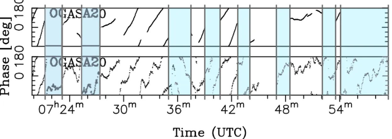
where Φ^r_raw is raw data fringe phase of the reference source, and Φ^r_v(U (t), V (t)) is the visibility phase calculated from the CLEAN components of the reference source image for a baseline with U (t) and V (t). N = 14 is the BBC number, M = 64 is the spectral channel number in the single BBC, ν₀^t is the RF frequency of the strongest H2O maser emissions in beam A, νn^r is the RF frequency at the lower band edge of the n-th BBC for the reference source as listed in Table 2.2, ∆ν = 250 kHz is the frequency spacing in the single BBC for the reference source, m is the integer number indicating the order of frequency channel in the single BBC, ∆τ_g^r(t) is the third-order polynomial fitting result of the temporal variation of the group delay obtained from the preceded fringe-fitting for the reference source. We refer to the phase calibration solutions obtained with this method as Direct Phase Transfer (DPT) solutions. The DPT solutions were then smoothed by making a running mean with the averaging time of 16 s in order to reduce the thermal noise. The smoothed DPT solutions are shown in Figure 2.6 as well as the one obtained with an ordinary AIPS phase referencing analysis (AIPS CL table), whose block diagram is shown in Figure 2.7. Note that the imaging process of J2339+6010 is common both in the DPT method (Figure 2.5) and the ordinary AIPS phase referencing analysis (this figure). Those two results are basically consistent with each other. Note that, even when solutions cannot be obtained with the fringe-fitting or the following AIPS self-calibration because of the signal-to-noise ratios (S/N) below a cutoff value, the DPT solutions were created from the raw fringe data, as shown for OGASA20 station in Figure 2.8. The final astrometric result with the smoothed DPT solutions is consistent with that with the AIPS CL table at epoch F.

Amplitude gain adjustment was performed using a third-order polynomial fitting for the amplitude self-calibration solutions for J2339+6010. Since S/N of J2339+6010 is unexpectedly low at epoch G, we could not obtain good solutions for J2339+6010 in the fringe-fitting. We therefore obtained the group delay solutions from 3C 454.3 and set the amplitude gain to the unity for all the observing time. The DPT solutions were created from the J2339+6010 fringe data together with the group delay solutions determined with 3C 454.3. At epoch I, since IRIKI did not attend the observation, we used the remained three stations in the data reduction.

(25)

2.3. DATA REDUCTION 15

2.3.3 Image Synthesis of PZ Cas

The Doppler shift in PZ Cas spectra due to Earth’s rotation and revolution was corrected after the phase referencing. The observed frequencies of the maser lines were converted to radial velocities with respect to LSR (Local standard of rest) using the rest frequency of 22.235080 GHz for the H2O 616_{− 5}23 transition. Since the cross power spectra within the received frequency region show a good flatness both in the phase and amplitude, the receiver complex gain characteristics was not calibrated in this analysis. We inspected the cross power spectra for all the baselines in order to select a velocity channel of the maser emission which would be unresolved and not have rapid amplitude variation. At this step, fast phase changes with a typical time scale of a few minutes to a few tens of minutes can be removed by the phase referencing, but slow time variations including a bias component as shown in Figure 2.9 cannot. The maser image was distorted because of the residual time variations of the fringe phase on a time scale of several hours, which might be caused by uncertainties in the updated VLBI correlator model. We conducted the fringe-fitting for the selected velocity channel with the solution interval of 20 min. We fitted the solutions to a third-order polynomial as shown in Figurer 2.9 and removed it from both of the fringe phases of PZ Cas and J2339+6010. This procedure can remove the residual fringe phase error from the PZ Cas data while it is transferred to the J2339+6010 data. As a result, this leads to an improvement of the PZ Cas image quality but in turn to a distortion of the J2339+6010 image. This distortion of the reference source causes an astrometric error in the relative position between the sources, as later discussed in Chapter 2.

2.3.4 Evaluation of Image Quality

Figure 2.9 also shows the fringe phase residuals obtained with the AIPS CL table. Al- though the fringe-fitting results with the AIPS CL table can be almost identifiable to those with the DPT solutions, it is later noted that the image peak flux density at VLSR = −42.0 km s⁻¹ with the DPT solutions is 2 % lower than that with the AIPS CL table at epoch F. In addition, the image root-mean-square noise resulting from the DPT solutions is 5 % higher than that resulting from the AIPS CL table. We can also see that the residual phases resulting from the DPT solutions in the fifth and sixth observing sessions in Figure 2.9 have a larger deviation than those resulting from the AIPS CL table. Although the number of the calibrated visibilities after applying the DPT amplitude is larger than that with the AIPS CL table, especially in the last two sessions, the visibilities with lower S/N might degrade the final image quality. We have to admit that the AIPS CL table may lead to a slightly higher quality in the image synthesis because the fringe-fitting and self-calibration take off visibility with low S/N. The problem is that

(26)

there were some observations whose data shows unexpectedly low S/N for certain baselines. For such cases, it was hard to create AIPS CL table with the fringe-fitting and self-calibration. From the following three reasons, we used the DPT solutions instead of the AIPS CL table for all the observing epochs: (1) the DPT is useful even when the fringe-fitting fails because of the low S/N; (2) the final astrometric results between the two methods have little difference; and (3) it is preferable to use a unified anaysis scheme for obtaining scientific results from a data set with the same (U , V ) distribution.

The DPT solutions and the long-term phase calibration data were applied to the remaining frequency channels to make image cubes for the LSR velocity range of −23.0 and −60.8 km s⁻¹ with the step of 0.2107 km s⁻¹. Image-synthesis with 60 µas pixel for a region of 4096 × 4096 pixels, roughly a 246 × 246-square milliarcsecond (mas) region, was made by using IMAGR. To initially pick up maser emissions in the maps, we used the AIPS 2-D Gaussian component survey task, SAD, in each velocity channel map in order to survey emissions. We visually inspected the surveyed Gaussian components one by one. We stored the image pixels larger than 5-σ noise level for a visually confirmed maser emission. Hereafter we define a maser “spot” as an emission in a single velocity channel, and a maser “feature” as a group of spots observed in at least two consecutive velocity channels at a coincident or very closely located positions.

2.3.5 Accuracy of the Relative Position of PZ Cas

In the phase referencing astrometric analysis, positions of the PZ Cas maser spots were obtained with respect to that of the J2339+6010 image. The positional error includes the effect of a peak position shift due to uncertainties in the VLBI correlator model (atmospheric excess path lengths (EPLs), antenna positions, EOP, and so on) for the sources. Hereafter we refer a relative position error of a pair of point sources using the phase referencing due to uncertainties in a VLBI correlator model as an astrometric error. We conducted Monte Carlo simulations of phase referencing observations for the pair of PZ Cas and J2339+6010 to estimate the astrometric error. For generating simulated phase referencing fringes, we used an improved version of a VLBI observation simulator, ARIS (Astronomical Radio Interferometer Simulator, Asaki et al. 2007), with new func- tions simulating station clocks (Rioja et al. 2012) and amplitude calibration errors. In the simulations, we assumed that flux densities of PZ Cas and J2339+6010 of equiva- lently 10 Jy and 0.2 Jy for 15.6 kHz and 224 MHz bandwidths, respectively, which were determined from our observations. The sources were assumed to be point sources. The observation schedule and observing system settings in the simulations such as the recording bandwidth and A/D quantization level were adopted from the actual VERA observations. A tropospheric zenith EPL error of 2 cm and other parameters were set as suggested for VERA observations (Honma et al. 2010). For simplification of the simulations, reference

(27)

2.4. RESULTS 17 source position errors were not considered. The simulation results from 200 trials are shown in Figure 2.10. They show that the 1-σ errors in the relative position are 72 and 33 µas in right ascension and declination, respectively. We used these standard deviations as the astrometric error in the following analysis.

At epoch I, IRIKI station geographically located at the center of the VERA could not attend the observation, so that the astrometric accuracy may become worse with the remaining three stations. We conducted another simulation series for the three-station case, and the resultant astrometric accuracy is 101 and 39 µas for right ascension and declination, respectively. We therefore use this astrometric accuracy at epoch I in the following analysis.

2.4 Results

Maser features of PZ Cas are spatially distributed over a region of 200 × 200 square mas. We identified 52 maser spots which are assembled into 16 maser features. Those maser features were arranged in 11 maser groups which are labeled from a to k as shown in Figure 2.11. The groups a to e, and g, h, i have radial velocity range between −51.9 and

−40.5 km s⁻¹. The groups f, j, and k which have been detected at one epoch have −52.3,

−39.3, and −37.6 km s⁻¹, respectively. The radial velocities of the identified maser spots are close to the stellar systemic velocity (VLSR = −36.16±0.68 km s⁻¹). Groups a and b located to the north and southeast of the spatial distribution, respectively, are bright and have complicated structures while the other groups (c to k) have a rather simple structure. For the following annual parallax analysis, we selected 16 maser spots among 52 using the following two criteria. (1) Maser spots are detected with the image S/N greater than or equal to 7. (2) The maser spot was detected at 8 epochs or more. All the selected maser spots belong to either group a or b by chance.

2.4.1 Annual parallax

In the first step of the annual parallax analysis we performed a Levenberg-Marquardt least-square model fitting of the maser motions with the same way as that described by Asaki et al. (2010) using the peak positions of the selected maser spots. We adopted the astrometric error as mentioned in Section 2.3 and a tentative value of a morphology uncertainty (a positional uncertainty due to maser morphology variation) of 50 µas in the fitting, equivalent to 0.1 AU by assuming the distance of 2 kpc to the source. Figures 2.12 and 2.13 show the images and the fitting results of all the selected maser spots. The stellar annual parallax, π^∗, was determined with the combined fitting with the Levenberg- Marquardt least-square analysis for all the selected spots. The obtained stellar annual

(28)

parallax is 0.380±0.011 mas at this stage.

If we carefully look at Figure 2.13, the maser spots do not seem to be properly identified with the image peak positions because multiple maser spots are spatially blended. This is caused when the multiple maser spots whose size is typically 1 AU (Reid & Moran 1981) are closely located comparing with the synthesized beam size of ∼ 1 mas in this case, equivalent to 2.6 AU at the distance of PZ Cas. To identify an individual maser spot properly, especially for blended structures, we performed AIPS JMFIT for the two- dimensional (2-D) multiple Gaussian component fitting of the emissions. Here we refer to a maser spot which can be identified with the image peak position as an isolated maser spot, and to a maser spot which cannot be identified with a single peak position because of the insufficient spatial resolution as a blended component. If we can identify 2-D Gaussian components using JMFIT, instead of SAD which automatically searches multiple spots, in the brightness distribution, we refer to such spots as identified spots. Figure 2.14 provides an example of the annual parallax least-square fitting for a maser spot using either the image peak position or the 2-D Gaussian peak. Table 2.4 lists our combined fitting results using the image peak only for the isolated spots, only for the blended components, and for all those involved in the two groups. We also tried to make another combined fitting using the Gaussian peak only for the isolated spots, only for the blended but identified spots with JMFIT, and all of them, as listed in the second column in Table 2.4. The combined fitting results for the isolated spots show little difference between the cases of image peak and Gaussian peak. On the other hand, the fitting result for the blended spots with JMFIT peak positions is definitely changed from that with the image peak for the blended components and become closer to that obtained with the isolated spots. If a maser spot is recognized as an isolated spot, in other words, if a maser cloud is spatially resolved into multiple spots in the image, the image peak position can be treated as the maser position. Figure 2.15 shows histograms of the selected 16 annual parallaxes using the image peak and Gaussian peak positions. We fitted the histograms to Gaussian curves. In the case of the image peak positions (left panel), a 1-σ of the Gaussian curve is 0.046 mas. On the other hand, the 1-σ for the case of the Gaussian peak position (right panel) is 0.039 mas. Because it seems that the water maser emissions of PZ Cas cannot be fully resolved and because the dispersion of the annual parallaxes using the Gaussian peak position is smaller than that using the image peak position, we adopted the Gaussian peak positions in our least-square model fitting. The model fitting results obtained from the individual spots are listed in Table 2.5. From the combined fitting analysis by using all the selected maser spots, we obtained the stellar annual parallax of 0.356 ± 0.011 mas with assumptions of the above astrometric error and morphology uncertainty at this stage.

Although maser features around RSGs are good tracers for astrometric VLBI during

(29)

2.4. RESULTS 19 several years (Richards, Elitzur, and Yates 2011) the morphology of the maser spots observed with the high resolution VLBI is no longer negligible for the precise maser astrometry. This monitoring observations of PZ Cas have been conducted quite so often for two years that we can investigate the contribution of the morphology uncertainty to the maser astrometry. Figure 2.16 shows the position residuals of the selected 16 maser spots after removing the stellar annual parallax of 0.356 mas, proper motion, and initial position estimated for each of the spots. The standard deviation of the residuals are 93 and 110 µas for right ascension and declination, respectively. Assuming that those errors have statistical characteristics of a Gaussian distribution, the morphology uncertainty is 59 ( =^√93²_{− 72}² ) and 105 ( =^√110²_{− 33}² ) µas for right ascension and declination, respectively, where 72 and 33 µas are the astrometric errors discussed in subsection 2.3.3. It is unlikely that the morphology uncertainty has different values between right ascension and declination, so that we adopt 105 µas as the morphology uncertainty on the safer side. Based on the trigonometric parallax of 0.356 mas, 105 µas is 0.29 AU at PZ Cas. We conducted the combined fitting with all the maser spots whose positions were determined with JMFIT, and obtained π^∗ of 0.356 ± 0.011 mas at this stage.

Note that the above error of the annual parallax is a result by considering the random statistical errors from the image S/N and the randomly changing maser spot position as well as a common positional shift to all the maser spots at a specific epoch due to the astrometric error. Because the majority of the maser spots and features in the current parallax measurement are associated with the maser group a, the obtained stellar annual parallax could be affected by a time variation of the specific maser features at a certain level. Assuming that all the 13 maser spots belonging to group a have an identified systematic error, the annual parallax error can be evaluated to be 0.011 ×^√13 = 0.040 mas. On the other hand, if we assume that maser spots belonging to a certain maser feature have a common systematic error but that some of them have their own time variations, the annual parallax error should be estimated to be somewhere ranging between 0.011 and 0.040 mas. To evaluate the contributions of such a systematic error, we carried out Monte Carlo simulations introduced by Asaki et al. (2010) for our astrometric analysis. First we prepared the imitated data set of the 16 maser spots with position changes added by considering the fixed stellar annual parallax and the maser proper motions. Secondly we added an artificial positional offset due to the image S/N, the astrometric accuracy, and the morphology uncertainty to each of the maser spot positions. The positional offset due to the image S/N was given to each of the maser spots at each epoch independently. The positional offset due to the astrometric error is common to all the maser spots at a specific epoch, but randomly different between the epochs. In this paper, we assumed that the positional offset due to the morphology uncertainty is common to all the maser spots belonging to a specific maser feature at a specific epoch, but randomly different

(30)

between the features and the epochs. We assume the standard deviation of the maser morphology uncertainty is 105 µas, equivalent to the intrinsic size of 0.29 AU. In a single simulation trial, we obtain the stellar annual parallax for the imitated data set. Thirdly we carried out 200 trials in order to obtain the standard deviation of the stellar annual parallax solutions. The resultant standard deviation is 0.026 mas which can be treated as the annual parallax error in our astrometric analysis. The resultant estimate of the stellar annual parallax is 0.356 ± 0.026 mas, corresponding to 2.81 ^+0.22⁻0.19 ^kpc.

2.4.2 Stellar Position and Proper Motion

Similar to the cases seen in other RSGs (VY CMa, Choi et al. 2008; S Per, Asaki et al. 2010; VX Sgr, Kamohara et al. 2005, Chen et al. 2006; NML Cyg, Nagayama et al. 2008, Zhang et al. 2012b), the maser features around PZ Cas are widely distributed over a 200 × 200 square mas (corresponding to 562 × 562 square AU at a distance of 2.81 kpc) while the velocity of the features (–52 to –37 km s⁻¹) are distributed more closely to the stellar systemic velocity than those found in other RSGs are. It is likely that the detected maser groups are located at the tangential parts of the shell-like circumstellar envelope, whose three dimensional velocity has a small line-of-sight velocity. We determined the proper motions of all detected maser spots identified at least in two epochs. Table 2.6 lists maser spots whose proper motions and positions were calculated with the stellar annual parallax determined above. Using the proper motion data listed in Tables 2.5 and 2.6, we then conducted the least square fitting analysis to obtain the position of PZ Cas and the stellar proper motion based on the spherically expanding flow model (Imai et al. 2011). The obtained stellar proper motion in right ascension and declination, µ^∗αcos δ=–3.7 ± 0.2 mas yr⁻¹ and µ^∗δ=–2.0 ± 0.3 mas yr⁻¹, respectively. The astrometric analysis result for PZ Cas is listed in Table 2.7. The proper motions of the detected maser spots are shown in Figure 2.17 together with the stellar position indicated by the cross mark.

(31)

2.4. RESULTS 21

Figure 2.1: Cas OB5 member stars. The abscissa is the Galactic latitude, and the ordinate is the Galactic longitude. The blue and red circles represent OB stars and RSGs, respectively. The blue and red filled circles represent the member stars listed in the Hipparcos catalogue. The background grey scale is the CO (J=1–0) map reported by Dame et al. (2001).

(32)

Figure 2.2: Conceptual illustration of the VERA. The VERA consists of four stations located at Mizusawa, Iriki,Ogasawara, and Ishigakijima. The maximum baseline is about 2300 km between Mizusawa and Ishigakijima. Each station has a radio telescope of 20 m diameter.

VERA Project/National Astronomical Observatory Japanc

(33)

2.4. RESULTS 23

Figure 2.3: Steward-mount dual-beam platform of the VERA antennas. VERA Project/National Astronomical Observatory Japanc

(34)

Figure 2.4: Time variation of system noise temperature at epoch F. The abscissa is time in UTC, and the ordinate is the system noise temperature in Kelvin. Dotted points are measurements, and the solid lines are the polynomial fitting curves after removing the abrupt changes. Left and right panels show beams A and B, respectively. From the top to bottom plot: MIZNAO20, IRIKI, OGASA20, and ISHIGAKI stations.

(35)

2.4. RESULTS 25

DPT

Imaging Initial

calibrations

Calibrated data Initial

calibrations

Tsys, Gain

Self- calibration

Digitizer in Particular

Delay calibrations J2339+6010

PZ Cas

Initial calibration Direct Phase Transfer

Figure 2.5: Block diagram of the Direct Phase Transfer (DPT) method for phase referencing VERA maser astrometry. The visibility phase, φν, because of the structure of the J2339+6010 image is subtracted based on the CLEAN components obtained in the imaging process as shown with the blue arrows.

(36)

Figure 2.6: Complex gain calibration solutions obtained from J2339+6010 at epoch F for the phase referencing. IRIKI is the reference antenna. Each antenna has two plots: the abscissa is time in UTC, and the ordinate is the phase calibration data in degree and the amplitude gain for the upper and lower plot, respectively. The left and right plots show the direct phase-transfer (DPT) solutions introduced in Chapter 2, and those obtained in an AIPS phase referencing analysis (AIPS CL table), respectively. For making the AIPS CL table, the solution intervals are set to two, two and ten minutes for the fringe-fitting, phase-only self-calibration, and amplitude- and-phase self-calibration, respectively. From the top to bottom plot: MIZNAO20, IRIKI, OGASA20, and ISHIGAKI.

(37)

2.4. RESULTS 27

Imaging J2339+6010

PZ Cas

Initial calibrations

Calibrated data Initial

calibrations

Tsys, Gain

Delay calibrations

Self- calibration

Threshols of S/R

Digitizer in Particular

Initial calibration

Figure 2.7: Block diagram of the ordinary AIPS phase referencing analysis to generate an AIPS CL table. In this thesis study, we adopted the S/N threshold of 6 to obtain complex gain solutions in the fringe-fitting and self-calibration.

(38)

Figure 2.8: Phase calibration data as shown in Figure 2.5, but only for OGASA20. The top plot shows AIPS CL table with the ordinary AIPS phase referencing analysis. The bottom plot shows the DPT data. Light blue area is missing phase data by the AIPS phase referencing analysis.

(39)

2.4. RESULTS 29

Figure 2.9: Phase solutions using the fringe-fitting with the solution interval of 20 min for the PZ Cas’s brightest velocity channel (VLSR = −42.0 km s⁻¹) at epoch F. The abscissa is the time in UTC, and the ordinate is the phase in degree. IRIKI is the reference antenna. The dotted points are the fringe-fitting solutions, and the solid lines represent fitting results with a third-order polynomial for each station. Left and right plots show the fringe-fitting results after the phase referencing with the direct phase transfer calibration and the AIPS CL table, respectively. From the top to bottom plot: MIZNAO20, IRIKI, OGASA20, and ISHIGAKI.

(40)

Figure 2.10: Astrometric observation simulation results for the pair of PZ Cas and J2339+6010. The dots represent PZ Cas’s image peak positions relative to J2339+6010 at 22 GHz with the VERA for 200 trials. The ellipses represent 1-σ for the distributions. Left: the VERA full array case. Right: the VERA three-station case (MIZNAO20, OGASA20, and ISHIGAKI).

(41)

2.4. RESULTS 31

Figure 2.11: Spatial distribution of the PZ Cas H₂O masers in the 12 epochs. The outlines of maser features represent a 5-σ noise-level contour (418, 722, 661, 367, 467, 344, 309, 658, 686, 440, 313, and 285 mJy at epoch A, B, C, D, E, F, G, H, I, J, K and L, respectively). The synthesized beams are shown in the upper 1×1-square mas boxes. Maser features srrounded with circles represent maser groups. Groups f , i , j , and k are features detected at a single epoch. Group a is composed of four features, Groups b and g are composed of two features. The map origin is the phase-tracking center.

(42)

Figure 2.12: Spatial motions of 10 isolated maser spots. Color represents an observation epoch as shown in Figure 2.11. Dotted lines represent the best fit annual parallax and proper motion. The outermost contours show a 5-σ noise level, and contours are increased by a factor of power of 2. The number at the left bottom corner in each of the panels is the maser spot ID as listed in Table 2.5. Positional errors are displayed at the image peak positions. Dashed lines represent the least-squar fitting results of the spatial motion of an annual parallax and a linear motion for the maser peak positions.

(43)

2.4. RESULTS 33

Figure 2.13: Same as Figure 2.12 but the maser spots identified as the blended component. The maser components in the upper two panels have two maser spots while the ones in the lower panels have a single spot.

(44)

Figure 2.14: Least-square fitting results of the motions of the maser spot with the LSR velocity of −42.2 km s⁻¹. Top two: least-square fitting using the image peak positions. Bottom two: least-square fitting using the two dimensional Gaussian peak positions. Left panels show the maser positions after removing the initial position and the proper motions.

(45)

2.4. RESULTS 35

Figure 2.15: Histograms of individual annual parallaxes for 16 maser spots. Left: histogram for the case that the maser spot positions are measured with the image peak positions. The solid line represent a Gaussian fitting curve with the histogram. The 1-σ of the Gaussian curve is 0.046 mas. Right: the same as the left panel but for the case that the maser spot positions were measured with the Gaussian peak positions, and the 1-σ is 0.039 mas.

(46)

Figure 2.16: Position residuals of the 16 maser spots after removing the annual parallax of 0.356 mas, proper motions, and initial positions. The abscissa represents the maser spot ID as shown in Figures 2.12 and 2.13, and the ordinate is the position residual in mas. For each epoch, the position residuals in right ascension and declination are shown in the upper and lower panel, respectively.

(47)

2.4. RESULTS 37

Figure 2.17: Internal motions of maser spots around PZ Cas. The cross bars around the map origin represent the position of PZ Cas and its positional error obtained the least square fitting. The color represents the radial velocity, and open circles and triangles are red- and blue-shifted maser spots with respect to the systemic velocity. Left: spatial distributions of the maser spots with respect to the stellar position (coordinate origin). Right upper: radial velocity – position plot. The abscissa is the angular distance from the stellar position, and the ordinate is the radial velocity difference from the systemic velocity. Right bottom: transverse velocity – position plot.

(48)

Table 2.1: Observing epochs of PZ Cas astrometric monitoring observations

Epoch Date Time range

(UTC) A 2006 Apr 20 19:41 – 05:20 B 2006 Jul 14 14:21 – 23:10 C 2006 Aug 13 12:21 – 21:35 D 2006 Oct 19 08:01 – 17:20 E 2006 Dec 13 04:21 - 13:40 F 2007 Mar 22 00:21 – 08:17 G^a 2007 May 2 18:51 – 04:40 H^b 2007 Jul 25 13:20 – 23:04 I ^c 2007 Sep 19 10:20 – 20:10 J 2007 Nov 7 07:20 – 17:10 K 2007 Dec 22 04:25 – 14:15 L 2008 May 12 19:00 – 04:50

a Signal-to-noise ratio for all the baselines were unexpectedly low.

b _T

sys data of ISHIGAKI was used as that of OGASA20.

c IRIKI did not attend the observation.