1
Evolutionary branching under multi-dimensional
evolutionary constraints
Hiroshi C. Ito (1, *) and Akira Sasaki (1, 2)
1) Department of Evolutionary Studies of Biosystems, SOKENDAI (The Graduate University for Advanced Studies, Hayama, Kanagawa 240-0193, Japan
2) Evolution and Ecology Program, International Institute for Applied Systems Analysis, Laxenburg, Austria
* Corresponding author: (hiroshibeetle@gmail.com)
2
Abstract
The fitness of an existing phenotype and of a potential mutant should generally depend on the frequencies of other existing phenotypes. Adaptive evolution driven by such frequency-dependent fitness functions can be analyzed effectively using adaptive dynamics theory, assuming rare mutation and asexual reproduction. When possible mutations are restricted to certain directions due to developmental, physiological, or physical constraints, the resulting adaptive evolution may be restricted to subspaces (constraint surfaces) with fewer dimensionalities than the original trait spaces. To analyze such dynamics along constraint surfaces
efficiently, we develop a Lagrange multiplier method in the framework of adaptive dynamics theory. On constraint surfaces of arbitrary dimensionalities described with equality constraints, our method efficiently finds local evolutionarily stable strategies, convergence stable points, and evolutionary branching points. We also derive the conditions for the existence of evolutionary branching points on
constraint surfaces when the shapes of the surfaces can be chosen freely.
1. Introduction
Individual organisms have many traits undergoing selection simultaneously, inducing their simultaneous evolution. At the same time, evolutionary constraints (i.e., trade-offs) often exist, such that a mutation improving one trait inevitably makes another trait worse (Flatt and Heyland, 2011), e.g., trade-off between speed and efficiency in feeding activity of a zooplankton species (Daphnia dentifera) (Hall et al., 2012). In those cases, the second trait may be treated as a function of the first trait. In such a manner, evolution of populations in multi-dimensional trait spaces may be restricted to subspaces with fewer dimensionalities. We call such subspaces� constraint surfaces �for�convenience,�although�they�may�be�one dimensional (curves), two dimensional (surfaces), or multi-dimensional (hyper- surfaces).
In adaptive dynamics theory (Metz et al., 1996; Dieckmann and Law, 1996), directional evolution along such a constraint surface can be analyzed easily by examining selection pressures tangent to the surface, which allows us to find evolutionarily singular points where directional selection along the surface
vanishes (deMazancourt and Dieckmann, 2004; Parvinen et al., 2013). On the other hand, evolutionary stability (Maynard Smith, 1982) and convergence stability (Eshel, 1983) of those singular points can be affected by the local curvature of the
3
surface. At present, analytical methods for examining both evolutionary and convergence stabilities have been developed for one-dimensional constraint curves in two-dimensional trait spaces (deMazancourt and Dieckmann, 2004; Kisdi, 2006) and in arbitrary higher-dimensional trait spaces (Kisdi, 2015). In this paper, we develop a Lagrange multiplier method that allows us to analyze adaptive evolution along constraint surfaces of arbitrary dimensionalities in trait spaces of arbitrary dimensionalities, as if no constraint exists. We focus on evolutionary branching points (points that are convergence stable but evolutionarily unstable), which induce evolutionary diversification through a continuous process called evolutionary branching (Geritz et al., 1997). Points of other kinds defined by combinations of evolutionary stability and convergence stability (e.g., points that are locally evolutionarily stable as well as convergence stable) can be analyzed in the same manner.
This paper is structured as follows. Section 2 contains a brief explanation of the basic assumptions of adaptive dynamics theory and a standard analysis of adaptive evolution along constraint surfaces. Section 3 presents the main
mechanism of our method in the case of one-dimensional constraint curves in two- dimensional trait spaces. In section 4, we describe a general form of our method for an arbitrary L-dimensional constraint surface embedded in an arbitrary M- dimensional trait space. In section 5, the conditions for existence of candidate branching points (CBPs) along constraint surfaces when their shapes can be chosen freely are derived. Section 6 shows two simple application examples. In section 7, we discuss our method in relation to other studies.
2. Basic assumptions and motivation
To analyze evolutionary dynamics, we use adaptive dynamics theory (Metz et al., 1996; Dieckmann and Law, 1996). For simplicity, we consider a single asexual population in a two-dimensional trait space � = , with two scalar traits and , in which all possible mutants �′ = ′, ′ are restricted to a constraint curve ℎ �′ = . The theory (sensu stricto) assumes sufficiently rare mutations and a sufficiently large population size, so that the population is monomorphic and almost at equilibrium density whenever a mutant emerges. In this case, whether a mutant can invade the�resident�population�can�be�determined�by�the�mutant s� initial per capita growth rate, called invasion fitness � �′; �∘ , which is a function of the mutant phenotype �′ and the resident phenotype �∘ = ∘, ∘ . The mutant can invade the resident only when � �′; �∘ is positive, resulting in substitution of the resident in many cases. Repetition of such a substitution is
4
called a trait substitution sequence, forming directional evolution toward greater fitness as long as the fitness gradient at the resident is not small. Under certain conditions, when the fitness gradient along the curve becomes small, a mutant may coexist with the resident, which may bring about evolutionary diversification into two distinct morphs, called evolutionary branching (Metz et al., 1996; Geritz et al., 1997, 1998). In this paper, we assume for simplicity that the population is
unstructured, although our results (Theorems 1–3) are also applicable to
structured populations, as long as reproduction is asexual and the invasion fitness function is defined in the form of � �′; �∘ .
Denoting points on the constraint curve by � � with a scalar parameter �, we can express the resident and mutant phenotypes as �∘ = �∘ , �∘ and
�′ = �′ , �′ , respectively. In this case, the evolutionary dynamics along the curve can be translated into that in a one-dimensional trait space �. The expected shift of the resident phenotype due to directional evolution can be described by an ordinary differential equation (Dieckmann and Law 1996):
d�∘
d =
�∘ ��
� �∘ , a
where �∘ is the equilibrium population density for a monomorphic population of
�∘, is the mutation rate per birth, �� is the root mean square of mutational steps �′− �∘, and
� �∘ = [�� ���′; �′ ∘ ]
�′=�∘ b
is the fitness gradient along the curve at the position where the resident exists (Eq. (1a) is specific to unstructured populations; see also Durinx et al. (2008) for a general form for structured populations). Here, �∘, , and ��, as well as � �∘ , may depend on �∘, although they are denoted without �∘ for convenience. In adaptive evolution, along the parameterized constraint curve, the conditions for evolutionary branching are identical to those for one-dimensional trait spaces without constraint (Metz et al., 1996; Geritz et al., 1997). Specifically, along the constraint curve, a point � = ( � , � is an evolutionary branching point, if it is (i) evolutionarily singular,
� � = a
(i.e., no directional selection for a population located at �), (ii) convergence stable (Eshel, 1983),
5
� ≡ [�g ���∘∘ ]
�∘=�
< b
(i.e., � is a point attractor in terms of directional selection), and (iii) evolutionarily unstable (Maynard Smith, 1982),
� ≡ [� � ���′′; �∘ ]
�′=�∘=��
> c
(i.e., for residents, �∘= �, � �′; � forms a fitness valley along �′ with its bottom
�′= � leading to disruptive selection). Eq. (2b) can be expressed alternatively by noting (1b) as
� = [���∘ �� ���′; �′ ∘
�′=�∘
]
�∘=��
= � + [� � ���′��′; �∘∘ ]
�′=�∘=��
< . d
However, in trait spaces with more than two dimensions, constraints may form surfaces or hyper-surfaces whose parametric expression may be difficult or complicated. To avoid such difficulty, we develop an alternative approach that does not require parametric expression of constraint spaces.
3. One-dimensional constraint curves in two-
dimensional trait spaces
The Lagrange multiplier method is a powerful tool for finding local maxima and minima of functions that are subject to equality constraints. In this section, we develop a method for adaptive dynamics under constraints in the form of Lagrange multiplier method. For clarity, we consider the simplest case: constraint curves ℎ �′ = in two-dimensional trait spaces � = , . The method is generalized to arbitrary dimensions in the subsequent section.
3.1. Notations for derivatives
For convenience, we introduce some notations for derivatives of functions by their vector arguments. For a function with a single vector argument, its derivative by that argument is denoted by ∇. For a function with more than one argument, its partial derivative by its argument is denoted by ∇ . The same rule applies for second derivatives. We express first and second derivatives of the constraint
6
function ℎ �′ and the fitness function � �′; �∘ (at an arbitrary point �) as follows. For ℎ �′ , we write the gradient and its transpose as
∇ℎ � = (
�ℎ �′
�ℎ �� ′′
� ′ )�′=�
,
∇ ℎ � = (�ℎ �′
� ′
�ℎ �′
� ′ )�′=�,
and the Hessian matrix as
∇∇ ℎ � = (
� ℎ �′
� ′
� ℎ �′
� ′� ′
� ℎ �′
� ′� ′
� ℎ �′
� ′ )�′=�
. c
For the fitness function � �′; �∘ , we write the first and second derivatives by �′ at the position where �∘ exists as
∇�′� �∘; �∘ = (
�� �′; �∘
� ′
�� �′; �∘
� ′ )�′=�∘
= �∘ , a
∇�′∇�′� �∘; �∘ = (
� � �′; �∘
� ′
� � �′; �∘
� ′� ′
� � �ʹ; �∘
� ′� ′
� � �ʹ; �∘
� ′ )�′=�∘
= �∘ . b
When � �′; �∘ is regarded as a fitness landscape in the space of mutant trait �′ under a fixed resident trait �∘, Eq. (4a) gives its local gradient, and rescaling of Eq. (4b) gives its local curvature at �∘ (when �∘ = , rescaling is not needed; i.e.,
�∘ gives the curvature along a unit vector ). In this paper, we refer to Eqs. (4a) and (4b) as fitness�gradient �and� fitness�curvature, respectively. For convenience, we introduce = � and = � . We also introduce another second derivative, , defined by the first derivative of
7
�∘ = (
�� �′; �∘
� ′
�� �′; �∘
� ′ )�′=�∘
≡ (
��
� ′ �∘; �∘
��
� ′ �∘; �∘ )
c
at �,
= ∇�∘ � = (
∂
� ∘
��
� ′ �∘; �∘
∂
� ∘
��
� ′ �∘; �∘
∂
� ∘
��
� ′ �∘; �∘
∂
� ∘
��
� ′ �∘; �∘ )
�′=�∘=��
, d
which describes variability of the fitness gradient at �, depending on �∘, and thus determines the convergence stability of � when it is evolutionarily singular. We refer to as� fitness�gradient-variability. Analogous to Eq. (2d), Eq. (4d) is alternatively expressed as
= + ∇�∘∇�′� �; � , e
where
∇�∘∇�′� �; � = (
∂
� ′
��
� ∘ �∘; �∘
∂
� ′
��
� ∘ �∘; �∘
∂
� ′
��
� ∘ �∘; �∘
∂
� ′
��
� ∘ �∘; �∘ )
�′=�∘=��
. f
3.2. Lagrange functions for fitness functions in two-
dimensional trait spaces
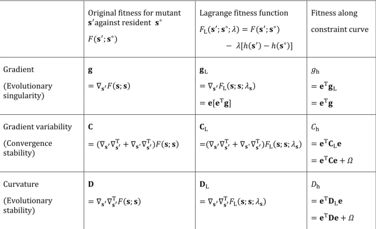
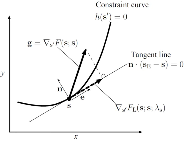
When no constraint exists, we can directly use , , and to check evolutionary singularity, convergence stability, and evolutionary stability of �, respectively. However, when possible mutants are restricted to the constraint curve ℎ �′ = , we need the elements of , , and along the curve to check those evolutionarily dynamical properties (Fig. 1). To facilitate such an operation, we integrate the fitness function � �′; �∘ and the constraint function ℎ �′ into
� �′; �∘; = � �′; �∘ − [ℎ �′ − ℎ �∘ ],
8
with a parameter . This function corresponds to the Lagrange function of
invasion fitness � �′; �∘ with a Lagrange multiplier , called the Lagrange fitness function in this paper. The second term is used to bind the population on the constraint curve. Here, the gradient of Lagrange fitness in �′ at � is
∇�′� �; �; = ∇�′� �; � − ∇ℎ �
= − |∇ℎ � |�,
where � = (� , � = ∇ℎ � |∇ℎ � |⁄ is the normal vector of the constraint curve at �. Thus, by choosing at
� = |∇ℎ � | =� ⋅ ∇ℎ � ⋅ ∇�
′� �; �
|∇ℎ � | ,
where the operator ⋅ indicates the inner product of the two vectors, the second term of Eq. (6) becomes the element of orthogonal to the curve (i.e., ∇ℎ � = [� ⋅ ]�). Consequently, Eq. (6) gives the tangent element of ,
∇�′� �; �; = − [� ⋅ ]�
= [� ⋅ ]�� ,
for any �, where � = (� , −� is the tangent vector of the curve at �. Note that the derivative of the second term of Eq. (5) subtracts the orthogonal element
∇ℎ � = [� ⋅ ]� from = [� ⋅ ]� + [� ⋅ ]�. Hence, the second term of Eq. (5), [ℎ �′ − ℎ �∘ ],�may�be�interpreted�as�a� harshness �of�the�constraint�on the organism, which removes the possibility of evolution orthogonal to the constraint curve, even if a steep fitness gradient exists in that direction.
3.3. Conditions for evolutionary branching along
constraint curves
When constraint curves in two-dimensional trait spaces have parametric
expressions, the conditions for � being an evolutionary branching point along the curves are given by Eq. (2). By using the Lagrange fitness function, we can express the left sides of those conditions into ones without parameters:
� � � = ∇�′� �; �; � , a
� = � [(∇�′∇�′+ ∇�∘∇�′ � �; �; � ]�� = ℎ, b
� = � [∇�′∇�′� �; �; � ]� = ℎ, c
9
where � (∇�′∇�′+ ∇�∘∇�′ � �; �; � = ∇�′∇�′� �; �; � + ∇�∘∇�′� �; �; � , and appropriate scaling of � is assumed so that | d �d� ,d �d� | = without loss of generality (Appendix A.3). Moreover, we have the following theorem for an arbitrary constraint curve described with h �′ = (see Appendix A.1–2 for the proof).
Theorem 1: Branching conditions along constraint (two-
dimensional trait spaces)
In two-dimensional trait space � = , �, a point � is an evolutionary branching point along the constraint curve ℎ � = , if � satisfies the following three conditions of the Lagrange fitness function Eq. (5) with Eq. (7):
(i) � is evolutionarily singular along the constraint curve ℎ � = , satisfying
∇�′� �; �; � = . a
(ii) � is convergence stable along the constraint curve, satisfying
h= � [(∇�′∇�′ + ∇�∘∇�′ � �; �; � ]� < . b (iii) � is evolutionarily unstable along the constraint curve, satisfying
h = � [∇�′∇�′� �; �; � ]� > . c
By Eq. (8), we can transform Eq. (10a) into
� ⋅ ∇�′� �; �� = ,
which may be easier to check. Table 1 summarizes how the fitness gradient, gradient variability, and curvature along the constraint curve are expressed in terms of the Lagrange fitness function.
3.4. Relationship with standard Lagrange multiplier
method
Since = �, defined by Eq. (7), can also be derived as the solution of condition (i), can be left as an unknown parameter satisfying condition (i), like a Lagrange multiplier in the standard Lagrange multiplier method. In this case, conditions (i) and (iii) are equivalent to the conditions for stationary points and local minima
second�derivative�test �in�the�standard method. When the fitness function is independent of resident phenotypes, h = h always holds. In this case, condition (ii) h < is never satisfied when condition (iii) h > holds. However, when the fitness function depends on resident phenotypes (i.e., frequency-dependent
10
fitness functions), satisfying condition (ii) is decoupled from not satisfying condition (iii). Thus, Theorem 1 is a modification of the standard Lagrange multiplier method to analyze frequency-dependent fitness functions by adding condition (ii) for convergence stability. In the standard method, h can be
examined with the corresponding bordered Hessian matrix (Eq. (22b)). Analogous calculations can be used to examine h (Eq. (22d)).
The above relationships hold also for the higher-dimensional constraint surfaces explained in the next section. Like the standard method, our method is completely analytical.
3.5. Effect of constraint curve curvature
Here, we explain how the curvature of the constraint curve affects the conditions for evolutionary branching (Eq. (10)). The curvature does not affect evolutionary singularity because Eq. (10a) is equivalent to Eq. (11), since it does not contain second derivatives of the constraint. On the other hand, convergence stability and evolutionary stability are both affected by the curvature, as previous studies have shown graphically (Rueffler et al. 2004; deMazancourt and Dieckmann, 2004) and analytically with parameterization (Appendix A in deMazancourt and Dieckmann, 2004; Kisdi, 2006). This feature is shown more clearly in our method without parameterization by transforming the left sides of Eqs. (10b) and (10c) into
h = � [(∇�′∇�′ + ∇�∘∇�′ � �; � ]� − � [ �∇∇ ℎ � ]�
= � � + ,
h = � � [∇�′∇�′� �; � ]� − � [ �∇∇ ℎ � ]�
= � � + ,
a
where, noting Eq. (7),
= −� [ �∇∇ ℎ � ]�
= ⋅ [−� ∇∇ ℎ � �|∇ℎ � | �] = ⋅ �.
b
The first terms in Eq. (12a), � � and � �, give fitness gradient variability and fitness curvature, respectively, for � along the curve when the constraint curve is a straight line. The effect of the constraint curvature is given by , which is the
11
inner product of the fitness gradient and a curvature vector � at �. The curvature vector is a scaled normal vector
� = ��� a
with
� = −� ∇∇ ℎ � �|∇ℎ � | , b
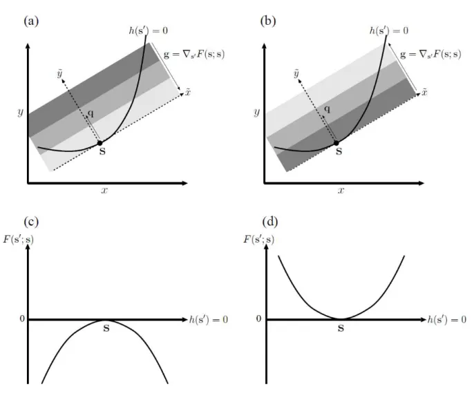
so that its length |�| is equal to the reciprocal of the curvature radius. Specifically, the constraint curve ℎ �′ = can be described locally with
̃′ = � ̃′ + O ̃′ , c
with the ̃- and ̃-axes given by �� and �, i.e., ̃′ = � ⋅ �′− � and ̃′= � ⋅
�′− � (Fig. 2a).
Note that h and h in Eq. (12a) have the same second term = ⋅ �. Thus, the effects of the curvature on h and h are large when the element of the fitness gradient orthogonal to the curve is large, as illustrated in Figure 2. If their directions, i.e., those of the fitness gradient and curvature vector, are opposite, the resulting negative curvature effect decreases both h and h (Fig. 2a), which makes the point � more convergence and evolutionarily stable (Fig. 2c).
Conversely, if they have the same direction, the resulting positive curvature effect increases both h and h (Fig. 2b), which makes the point � less convergence and evolutionarily stable (Fig. 2d). When results in negative h and positive
h simultaneously, � is an evolutionary branching point along the constraint curve. Note that even when the original two-dimensional fitness landscape is flat, i.e., = , the fitness landscape along the constraint curve has a curvature h= Ω when Ω ≠ . In this sense, we refer to as apparent fitness curvature.
4. Extension to higher dimensionalities
In this section, we extend the two-dimensional method discussed above for higher dimensionalities. We consider an arbitrary M-dimensional trait space � =
, … , and an invasion fitness function � �′; �∘ . For an arbitrary position �, the fitness gradient, fitness gradient variability, and fitness curvature are written in the same manner as the two-dimensional case:
12
= ∇�′� �; � ,
= ∇�′∇�′� �; � + ∇�∘∇�′� �; � = ∇�′∇�′+ ∇�∘∇�′ � �; � ,
= � ∇�′∇�′� �; � .
We consider an arbitrary L-dimensional constraint surface defined by ℎ �′ = for = + , , , to which all possible mutants �′ are restricted. To analyze adaptive evolution along the constraint surface, we obtain the elements , , and
along the surface as follows.
4.1. Lagrange fitness function for constraint surface
As described in Lemma 2 in Appendix C, the Lagrange fitness function for the constraint surface is constructed as
� �′; �∘; � = � �′; �∘ − ∑ [ℎ �′ − ℎ �∘ ]
= +
,
with � � = + , … , . When the normal vectors � = ∇ℎ �� |∇ℎ � |⁄ � for
= + , , are orthogonal, we can choose
� = � ⋅
|∇ℎ � |� ,
such that the gradient of the second term of Eq. (15) with respect to �′ gives the element of orthogonal to the surface,
∑ λ�
= +
∇ℎ � = ∑ [� ⋅ ]�
= +
.
Thus, the gradient of Eq. (15) gives the tangent element of ,
∇�′� �; �; �� = − ∑ [� ⋅ ]�
= +
= ∑[� ⋅ ]�
=
= ,
where = � , , � are the tangent vectors of unit lengths, which are chosen to be orthogonal (e.g., with Gram–Schmidt orthonormalization) without losing
generality.
13
Even in general cases where the normal vectors may not be orthogonal, we can make ∇�′� �; �; �� = ∑ [� ⋅ ]�= hold [Eq. (C.15) in Appendix C] by choosing � at
�� = +∇�′� �; � = + ,
where + = [ ]− is the pseudo inverse of = (∇ℎ + � , , ∇ℎ � , i.e.,
+ gives the − -dimensional identity matrix − . In statistics, �� is the regression coefficients for predictor variables ∇ℎ + � , , ∇ℎ � , to explain . When the normal vectors are orthogonal, Eq. (19) yields Eq. (16).
4.2. Conditions for the existence of CBPs along
constraint surfaces
The dimensionalities of constraint surfaces can be greater than one, in which case one-dimensional conditions for evolutionary branching cannot be applied. As for multi-dimensional conditions for evolutionary branching, numerical simulations of adaptive evolution in various eco-evolutionary settings (Vukics et al., 2003;
Ackermann and Doebeli, 2004; Egas et al., 2005; Ito and Dieckmann, 2012) have shown that evolutionary branching arises in the neighborhood of a point �, if � is (i) evolutionarily singular, (ii) strongly convergence stable (Leimar, 2005, 2009), and (iii) evolutionarily unstable. Among these three conditions, conditions (i) and (iii) are simply extensions of conditions (i) and (iii) in the one-dimensional case [Eq. (2)], respectively. Condition (i) means the disappearance of the fitness gradient for the resident located at �, and condition (iii) means that the fitness landscape is concave along at least one direction. On the other hand, condition (ii) introduces the�new�term� strongly�convergence�stable, �which�means�convergence� stability under any genetic correlation in the multi-dimensional mutant phenotype (see Leimar, 2005 for the proof of strong convergence stability).
Currently, no formal proof has determined whether the existence of points satisfying (i–iii) is sufficient for evolutionary branching to occur in the
neighborhood of those points, although substantial progress has been made (see section 7). In this paper, we refer to points satisfying (i–iii) as CBPs (candidate branching points). By applying the three conditions for CBPs, we establish the following multi-dimensional conditions for CBPs along the constraint surface (see Appendix C for the proof).
14
Theorem 2: Conditions for existence of CBPs along constraints
(multi-dimensional)
In an arbitrary M-dimensional trait space � = , , , a point � is a CBP (i.e., a point that is strongly convergence and evolutionarily unstable) along an arbitrary L-dimensional constraint surface defined by ℎ � = for = + , , , if � satisfies the following three conditions of the Lagrange fitness function Eq. (15) with Eq. (19):
(i) � is evolutionarily singular along the constraint surface, satisfying
∇�′� �; �; �� = . a
(ii)� � is strongly convergence stable along the constraint surface, i.e., the symmetric part of an L-by-L matrix
h = [ ∇�′∇�′ + ∇�∘∇�′ � �; �; �� ] � b
is negative definite, where an M-by-L matrix = � , , � consists of orthogonal base vectors � , … , � of the tangent plane of the constraint surface at �.
(iii) � is evolutionarily unstable along the constraint surface, i.e., a symmetric L-by-L matrix
h = ∇�′∇�′� �; �; �� � c
has at least one positive eigenvalue.
Analogous to the two-dimensional case, we can transform Eq. (20a) using Eq. (18) into
∇�′� �; � = . d
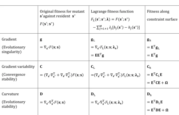
Table 2 summarizes how the fitness gradient, gradient variability, and curvature along the constraint surface are expressed in terms of the Lagrange fitness function.
4.3. Bordered second-derivative matrix
In the standard Lagrange multiplier method, whether an extremum is maximum, minimum, or saddled along the constraint surface can be examined with the corresponding bordered Hessian matrix (Mandy, 2013), in which calculation of , the base vectors of the tangent plane, is not needed. This technique is also useful for examining not only h, but also h, as explained below. For convenience, we denote the number of equality constraints by = − . In this paper, we define the bordered Hessian for h by a square matrix with size + ,
B = ( − ) , a
15
where = ∇ℎ + � , , ∇ℎ � , = ∇�′∇�′� �; �; �� , and trait axes are permutated appropriately so that separation of � = , , into =
, , and = + , , makes an × matrix
(∇ ′ℎ + � , , ∇ ′ℎ � nonsingular. Note that is multiplied by�− , which differentiates it slightly from the standard bordered Hessian, but simplifies the analysis of evolutionary stability along the surface (i.e., negative definiteness of
h= ). Similarly, to analyze strong convergence stability along the surface, we define a bordered second-derivative matrix
B = ( − / + ) , b
where = ∇�′∇�′+ ∇�∘∇�′ � �; �; �� . Then, we have the following two corollaries (see Appendix E for the derivation).
Corollary 1: Evolutionary stability condition by bordered
Hessian
A point � satisfying Eq. (20a) is locally evolutionarily stable along the constraint surface described in Theorem 2 (i.e., ℎ is negative definite) if every principal minor of of order = + , , + has the sign
− , where = − , and the th principal minor of is given by the determinant of the upper left × submatrix of ,
| B | = | B, ⋱ B,
B, … B,
| . a
Conversely, � is evolutionarily unstable along the constraint surface (i.e.,
ℎ has at least one positive eigenvalue) if Eq. (22a) for either of = + , , + has a sign other than − . For one-dimensional constraint curves in two-dimensional trait spaces ( = , = ),
h = � |∇ℎ � | .| B| b
Corollary 2: Strong convergence stability condition by
bordered second-derivative matrix
A point � satisfying Eq. (20a) is strongly convergence stable along the constraint surface described in Theorem 2 (i.e., ℎ has a negative definite symmetric part) if every principal minor of of order = +
, , + has the sign − , where = − , and the th principal minor of is given by
16
| B | = | B, ⋱ B,
B, … B,
| . c
For one-dimensional constraint curves in two-dimensional trait spaces ( = , = ),
h = � |∇ℎ � | .| B| d
4.4. Effect of constraint surface curvature
The fitness landscape along the constraint surface is affected by the curvature of the surface, similar to the two-dimensional case. For example, if the surface curves along a tangent vector � in the direction of original fitness gradient , as in Fig. 2b with � = � (̃-axis), the curvature makes the fitness landscape along � more concave, as in Fig. 2d. Specifically, Eqs. (20b) and (20c) are transformed to
h = [(∇�′∇�′ + ∇�∘∇�′ � �; � ] − ∑ � ∇∇ h �
= +
= + �,
h = [∇�′∇�′� �; � ] − ∑ �
= +
∇∇ ℎ �
= + �,
a
where the first terms in Eq. (23a), and , give fitness gradient variability and fitness curvature, respectively, for � along the surface when the surface is locally flat. The effect of the constraint curvature, i.e., apparent fitness curvature, is given by an -by- matrix
� = − ∑ �
= +
∇∇ ℎ � . b
This effect can be expressed as a kind of inner product of the fitness gradient and local curvature of the constraint surface, analogous to the two-dimensional case (Eq. (12b); Appendix F).
17
5. Potential for evolutionary branching
The method described in the above sections is used to find CBPs under given constraint surfaces. In this section, we consider cases in which we can freely choose dimensions and shapes. With this freedom, we can adjust h and h in Eq. (23a) using the apparent fitness curvature �, such that the point � becomes a CBP. By applying this operation to all points in a trait space, we can examine
whether the trait space has CBPs by choosing an appropriate constraint surface. This type of analysis was originally developed for one-dimensional constraint curves in two-dimensional trait spaces using graphical approaches (Bowers et al. 2003, 2005; Rueffler et al. 2004; de Mazancourt and Dieckmann 2004) and analytical approaches with parameterization (de Mazancourt and Dieckmann 2004; Kisdi 2006; Geritz et al. 2007). The latter approach has been extended further for one-dimensional constraint curves in trait spaces of arbitrary
dimensions (Kisdi 2015). Here, we extend this analysis for constraint surfaces with arbitrary dimensions by using Theorem 2 from above.
The basic idea is as follows. For an arbitrary point �, we first adjust � in Eq. (23a) so that the symmetric part of h becomes a zero matrix (i.e., neutrally convergence stable). If the largest eigenvalue of h is still positive (evolutionarily unstable), then we can slightly adjust � so that the symmetric part of h
becomes slightly negative definite (strongly convergence stable) while the largest eigenvalue of h remains positive. This operation is possible whenever
− > holds for some vector orthogonal to the fitness gradient . More specifically, we have the following theorem (see Appendix G for the proof).
Theorem 3: Potential for evolutionary branching
For a fitness function � �′; �∘ � defined on an arbitrary -dimensional trait space � = , , , if a point � satisfies the branching potential condition: the symmetric -by- matrix
= [ + ] � a
has at least one positive eigenvalue, then � is a CBP (a point that is
strongly convergence stable and evolutionarily unstable) along an − - dimensional constraint surface, given by
ℎ �′ = [�′− �]
� + [�′− �] [ + + ɛ̃ ] [�′− �] + O |�′− �| = ,� � � b with a positive �̃ that is smaller than the maximum eigenvalue of �, where
18
= − | | ,
= − = −∇�∘∇�′� �; � ,
= ∇�′� �; � ,
= ∇�′∇�′� �; � + ∇�∘∇�′� �; � .
� � c
The dimensionality of the constraint surface can be reduced arbitrarily by adding appropriate equality constraints.
In this paper, we refer to the matrix as the branching potential matrix. The branching potential condition is also expressed as > for some vector orthogonal to (because > gives > , which is sufficient for to have at least one positive eigenvalue). This ensures the coexistence of two slightly different phenotypes in the neighborhood of �, i.e., � � ; � > and
� � ; � > for � = � + � and � = � − � for positive and sufficiently small
�.
Analogous to Corollaries 1 and 2 in the previous section, we can translate Theorem 3 to one based on a bordered second-derivative matrix
B =
− / + , d
with = −∇�∘∇�′� �; � = −∇�∘∇�′� �; � = , as follows.
Corollary 3: Branching potential condition by bordered second-
derivative matrix
A point � is a CBP (a point that is strongly convergence stable and
evolutionarily unstable) along an − -dimensional constraint surface, given by Eq. (24b), if either principal minor of �
| B | = | B, ⋱ B,
B, … B,
| . e
of order = , , + has a sign other than −1.
19
6. Examples
In this section, we show two application examples with explicit formulation of invasion fitness functions built from resource competition. In the first example, we show how our method works by analyzing a simple two-dimensional case. Then, we analyze its higher-dimensional extension in the second example.
6.1. Example 1: Evolutionary branching along a
constraint curve in a two-dimensional resource
competition model
Model
We consider a two-dimensional trait space � = , , which is treated as a two- dimensional niche space with two niche axes and . We assume a constraint curve
ℎ �′ = ′ − ′ + = ,
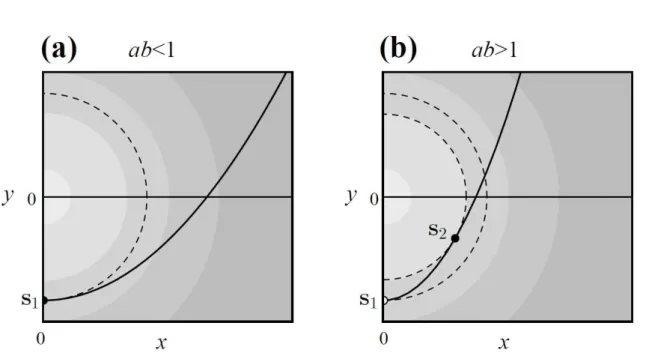
which is a parabolic curve ′ =� ′ − with two constant parameters and (solid curves in Fig. 3).
The invasion fitness function is constructed in the two-dimensional
MacArthur–Levins resource competition model (Vukics et al., 2003), explained below. When there exist N-phenotypes, the th�phenotype s�growth�rate�is�defined� by the Lotka–Volterra competition model,
��
� = � [ − ∑
(� ; � �
= �
] , a
where carrying capacity � of � and the competition effect � ; � on � from � are both given by two-dimensional isotropic Gaussian distributions
� = exp −|� |
� ,
(� ; � = exp −(|� − � |�
α ,
� � b
where � has its peak at the origin with standard deviation � , and
� ; � has its peak 1 at � = � with standard deviation �α, i.e., the competition effect decreases with their phenotypic distance. As this model and the constraint curve Eq. (25) are both symmetric about the -axis, we focus only on positive without loss of generality.
20
Analysis of evolutionary branching
We suppose a resident �∘ and a mutant �′ with population densities �∘ and �′, respectively. The invasion fitness � �′; �∘ of �′ against �∘ is defined by its initial growth rate (i.e., when �′ is very small) in the resident population at equilibrium density �∘= �∘ ,
� �′; �∘ = �lim′→+ [�′d�d ]′
�∘= �∘
= − �′; �∘�′ �∘ .
The first and second derivatives of this fitness function at an arbitrary point � give
= ∇�′� �; � = −� ,
= ∇�′∇�′� �; � = [�α −� ] −� ( ) ,
= (∇�′∇�′+ ∇�∘∇�′ � �; � = −� , and the derivatives of the constraint curve
∇ℎ � = − ,
∇∇ ℎ � = − give its normal, tangent, and curvature vectors at �
� = ∇ℎ �
|∇ℎ � | = √ +
− ,
� = √ + ,
� = −� ∇∇ ℎ � �
|∇ℎ � | � = √ + �.
�
The Lagrange fitness function is constructed as
� �′; �∘; � = � �′; �∘ − �[ℎ �′ − ℎ �∘ ]
= − �′; �∘�′ �∘ − �[ℎ �′ − ℎ �∘ ]
� a
with
21
�= ∇ℎ � ⋅|∇ℎ � | =� −+ . b
To apply Theorem 1, we calculate ∇�′� �; �; , h, and h as
∇�′� �; �; � = − �∇ℎ � = − +
� + � ,
h= � [ − �∇∇ ℎ � ]� =
� [
−
+ − ] ,
h = � [ − �∇∇ ℎ � ]��
= � [
�
�α − −�
+
+ +
− + ] .
h and h can also be obtained from bordered second-derivative matrices [Eqs. (22b) and (22d)].
By condition (i) in Theorem 1, the condition for evolutionary singularity along the curve is given by
∇�′� �; �; � = −� + + = ,
which yields two singular points
� = − , � =
(
√ −
− )
(� and � can also be obtained by Eq. (11), which may be easier). � can exist only when > . The condition > is understood as follows. The radius of the curvature of the constraint curve, given by /|�|, has its minimum / at � , whereas that of its tangential contour curve of � , + = , is constant . Thus, they have only a single tangent point � for / > (Fig. 3a), but two tangent points � and � for / < (Fig. 3b).
Condition (ii) in Theorem 1 applied to each of two singular points defined above gives the conditions for their convergence stability along the constraint curve,
h =� − < , a
h = −� −− < , b
22
respectively, and condition (iii) gives the conditions for their evolutionary instability along the curve,
h = � α −
−
� > , a
h = �
α +� [ − − ] > , b
respectively. Clearly, when < , the unique singular point � is always
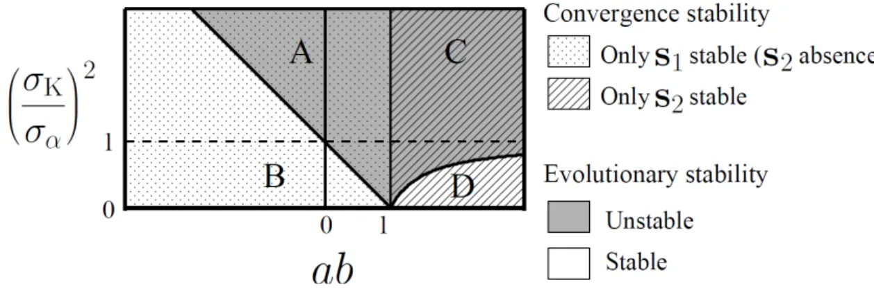
convergence stable. Moreover, this point is an evolutionary branching point as long as is sufficiently close to 1, because Eq. (36a) is transformed into
(��
α) > − a
(region A in Fig. 4). When > , there exist two singular points � and � , in which case � is always convergence stable while � never is. By Eq. (36b), � is an evolutionary branching point when
(��
α) > − − b
(region C in Fig. 4).
Notice that evolutionary branching points exist even for � /�α < as long as is sufficiently close to 1 (i.e., when the constraint curve and its tangential contour of � have sufficiently similar curvature radii of at � ). Conversely, when the constraint curve is a straight line ( = ), evolutionary branching points can exist only when � /�α > , equivalent to the case of one-dimensional trait spaces with no constraint (Dieckmann and Doebeli, 1999).
6.2. Example 2: Potential for evolutionary branching
through resource competition in multi-dimensional
trait spaces
We generalize the above two-dimensional model and apply the branching potential condition to determine whether each point in the trait space can become a CBP when we freely choose the shape of the constraint surface.
Model
We consider an arbitrary M-dimensional trait space � = , , , where the growth rate of phenotype � is given by the same equation used for two-
dimensional resource competition [Eq. (26a)], which gives the same form of the invasion fitness function
23
� �′; �∘ = �lim′→+ [�′��� ]′
�∘= �∘
= − �′; �∘�′ �∘ .
Unlike the two-dimensional case, we do not define explicit forms for the carrying capacity distribution � and competition kernel �′; �∘ . We assume that those functions are both smooth. For the competition kernel, we assume that
�∘; �∘ = , and that competition strength is determined by the relative phenotypic difference of �′ from �∘, i.e., �′; �∘ can be treated as a function with a single argument �′ − �∘,
�′; �∘ = ̃ �′− �∘ . a
We also assume that the strength of competition is maximal between identical phenotypes, i.e.,
∇�′ �∘; �∘ = , b
and the symmetric matrix
∇�′∇�′ �∘; �∘ c
is negative definite for any �∘. For example, the Gaussian competition kernel in the two-dimensional model given by Eq. (26b) fulfills these conditions.
Potential for evolutionary branching
At an arbitrary point �, the first and second derivatives of the invasion fitness are obtained as
= ∇�′� �; � = ∇ln � ,
= ∇�′∇�′� �; � + ∇�∘∇�′� �; � = ∇∇ ln � ,
= ∇�′∇�′� �; �
= −∇�′∇�′ �; � + ∇∇ ln � − ∇ln � ∇ ln � ,
= −∇�∘∇�′� �; � = −
= −∇�′∇�′ �; � − ∇ln � ∇ ln �
(Appendix H). Then, by the branching potential condition in Theorem 3, we can quickly examine whether an arbitrary point � has potential for being a CBP. In this model, the branching potential matrix (Eq. (24a)) is calculated as
24
= [ + ] = − [∇�′∇�′ �; � + ]
= − ∇�′∇�′ �; � +
= − ∇�′∇�′ �; � ,
where = = [ − /| | ] = − = is used. As ∇�′∇�′ �; � is assumed to be negative definite, Eq. (41) is positive semidefinite, i.e.,� is zero for ∝ , or positive otherwise. Thus, Eq. (41) has − positive eigenvalues and a single zero eigenvalue in the direction of . Therefore, any � can become a CBP with the appropriate choice of local dimensionality and shape of the
constraint surface around the point. Such a constraint surface is given by substituting Eq. (40) into Eq. (24b), yielding
ℎ �′ = [∇ln � ] [�′− �]
� + [�′− �] [∇∇ ln � + ɛ̃ ][�′− �] + O |�′− �|
= � �′ + ɛ̃|�′− �| + O |�′− �| = ,
� � � a
which gives
∇ℎ � = ∇ln � ,
∇∇ ℎ � = ∇∇ ln � + ɛ̃ ,� b
with a positive and sufficiently small ɛ̃. In other words, for an ( − )-
dimensional constraint surface with a tangent point � of an isosurface of � , if the constraint surface has slightly weaker curvature (by ɛ̃) than the isosurface at
�, then � is a CBP along the surface, as illustrated in Figure 5.
Multi-dimensional Lagrange multiplier method
Although Appendix G proves that Eq. (42) makes � become a CBP along the constraint surface in a general way, here we directly apply Theorem 2 to Eq. (42) and show how this theorem works. As the constraint surface has only a single equality condition ℎ �′ = , the Lagrange fitness function [Eq. (15)] for a focal point � becomes
� �′; �∘; � = � �′; �∘ − �[ℎ �′ − ℎ �∘ ], with a scalar � given by Eq. (19)
� = +∇�′� �; � =| ln � | ∇ln � =∇ ln � ,
25
where = ∇ℎ � and + = [ ]− = ∇ ℎ � /|∇ℎ � | = ∇ ln � /
|∇ln � ∣ are column and row vectors, respectively. As for the choice of base vectors for the tangent plane of the constraint surface, we can use the eigenvectors corresponding to positive eigenvalues of the branching potential matrix [Eq. (41)] as the orthogonal base vectors, = � , … , � − , satisfying � ⋅ � = for all =
, … , − , where � = ∇ℎ � /∣ ∇ℎ � ∣ is the normal vector of the surface. Then, by condition (i) in Theorem 2, any � is evolutionarily singular along the surface, as it satisfies
∇�′� �; �; � = ∇ln � − �∇ℎ �
= ∇ln � − ∇ln � = . a
As for condition (ii), we calculate
h = [ − �∇∇ ℎ � ]
= [∇∇ ln � − ∇∇ ln � − ɛ̃ ]
= −ɛ̃ = −ɛ̃ − .
b
Thus, [ h+ h] = h= −ɛ̃ − is always negative definite with positive ɛ̃, in which case � is always strongly convergence stable along the constraint surface. Condition (iii) gives its evolutionary stability condition
h = [ − �∇∇ ℎ � ]
= − [∇�′∇�′ �; � + ∇ln � ∇ ln � + ɛ̃ ]
= − [∇�′∇�′ �; � + ɛ̃ ] ,
c
where ∇ln � = = is used. As ∇�′∇�′ �; � is negative definite by definition, h is positive definite for sufficiently small ɛ̃. Therefore, � is a CBP along the constraint surface for positive and sufficiently small ɛ̃. As h and h are negative definite and positive definite, respectively, in this case, any smooth subspace of this constraint surface that contains � also has a CBP at �.
7. Discussion
7.1. Extension of Levins’ fitness set theory
Adaptive evolution is multi-dimensional in nature, and it is a widespread phenomenon that evolutionary constraints (e.g., due to genetic, developmental, physiological, or physical constraints) restrict directions that allow mutants to emerge or to have sufficient fertility (Flatt and Heyland, 2011). For example,
26
genotypes of a zooplankton species (Daphnia dentifera) illustrate the trade-off between feeding speed and efficiency (Hall et al., 2012). This situation may be proximately due to genetic or developmental systems, but it might ultimately be imposed by physical laws because no system can maximize power and efficiency at the same time under the second law of thermodynamics. Due to those constraints, an evolutionary trajectory induced by selection may be bounded on subspaces with fewer dimensionalities (e.g., selection responses of butterfly wing spots (Allen et al., 2008)). If such a subspace, i.e., a constraint surface, is parameterized so that coordinates on the surface are described with those parameters, adaptive evolution along the surfaces can be translated into adaptive evolution in the parameter space without constraint. In such a case, conventional analysis of parameters such as directional selection, evolutionary stability, and convergence stability can apply directly. However, parameterization may be difficult or
complicated when the constraint surfaces are multi-dimensional.
Levins (1962, 1968) developed a geometric method for the analysis of adaptive evolution along constraint curves (or surfaces), which does not require their parameterization. This method, known as �evins �fitness set theory, can be used to analyze directional evolution and evolutionarily stable points along
constraint curves by examining how the contours of fitness landscapes in the trait spaces cross or are tangent to the constraint curves. A limitation of this method is that fitness functions are assumed to be independent of existing resident
phenotypes, i.e., frequency-independent, despite the expectation of such
dependency in fundamental ecological interactions (e.g., resource competition, predator–prey interactions, mutualism) (Dieckmann et al., 2004). In this case, the resulting static fitness landscape cannot induce evolutionary branching (Metz et al., 1996; Geritz et al., 1997, 1998), although evolutionary branching is thought to be an important ecological mechanism for the evolutionary diversification of biological communities (Dieckmann et al., 2004).
Recently,��evins �method�has been extended to the analysis of frequency- dependent fitness functions for one-dimensional constraint curves in two- dimensional trait spaces (Rueffler et al. 2004; deMazancourt and Dieckmann, 2004; Bowers et al. 2005). The extended method can be used to analyze evolutionary branching along constraint curves by examining convergence stability as well as the evolutionary singularity and stability of focal points.
In this paper, we further developed the extension of �evins �method described above to analyze constraint surfaces of arbitrary dimensionalities in the form of Lagrange multiplier method. As our Lagrange multiplier method is completely analytic, one can easily use it to analyze adaptive evolution along constraint