Space-time Horizons
Sen Zhang
DOCTOR OF PHILOSOPHY
Department of Particle and Nuclear Physics
School of High Energy Accelerator Science
The Graduate University for Advanced Studies
2010
In this Thesis I discuss quantum fluctuations in physics of horizons. There are two main topics. The first topic is the fluctuations in Unruh effect. When a particle uniformly accelerated in Minkowski vacuum, it will experience the vacuum as a thermal bath. Using a stochastic approach, we investigated the fluctuations of this particle and proved the equipartition theorem for the transverse fluctuations. We also obtained the relaxation time of the fluctu- ations and the radiation due to the fluctuations(the Unruh radiation [12]). These result are also related to the experiment for detecting the Unruh effect by using high intensity laser(ELI) which is under construction in Europe now. The second topic is to apply fluctuation theorem to black holes. There is an analogue between black hole physics and thermodynamics. This analogue was well established in equilibrium region. We investigated the fluctuations of the black holes. We considered a system with a black hole coupled with matter fields and derive a non-equilibrium relation for the black holes. This relation corresponds to the non-equilibrium fluctuation theorem of Crooks and Jarzynski. As a result, we can also obtain the generalized second law from this relation. In our derivation, the second law holds only after taking a thermodynamic average, and it should be violated as individual process in a way to satisfy the Jarzynski equality. The thermodynamic features of the horizons should be closed related to a more fundamental structure of space- time. So it will be important to investigate the fluctuations of the horizons.
ii
Abstract ii
1 Introduction 1
2 Physics of Horizons 4
2.1 Unruh Effect . . . 4
2.1.1 Scalar Fields in curved space . . . 4
2.1.2 Rindler Space . . . 7
2.2 Black Hole Physics . . . 10
2.2.1 Black Hole Thermodynamics . . . 11
2.2.2 Hawking Radiation . . . 13
2.2.3 Information Puzzle . . . 16
2.3 The Argument of Ted Jacobson . . . 16
2.4 Membrane Paradigm . . . 19
2.4.1 The Electromagnetic Membrane . . . 20
2.4.2 The Gravitational Membrane . . . 22
3 Stochastic Approach to Unruh Radiation 32 3.1 Detectability of Unruh Effect . . . 32
3.2 Unruh Detector . . . 35
3.2.1 1+1 Dimensions . . . 36
3.2.2 3+1 Dimensions . . . 38
3.3 Stochastic Equation of an Accelerated Particle . . . 42 iii
3.6 Thermalization in Electromagnetic Field . . . 63
3.7 Summary . . . 65
4 Fluctuation Theorem and Black Hole 67 4.1 Jarzynski Equality and Fluctuation Theorem . . . 68
4.1.1 Jarzynski Equality . . . 68
4.1.2 Fluctuation Theorem . . . 70
4.2 Application to Black Holes . . . 72
4.2.1 Transition Rates . . . 73
4.2.2 Non-equilibrium Fluctuations of Horizons . . . 75
4.3 Future Work . . . 78
A Radiation Damping 81 A.1 Abraham-Lorentz-Dirac Force . . . 82
A.2 Landau-Lifshitz Equation . . . 87
References 88
iv
Introduction
One of the most interesting problem for theoretical physics must be the unification of quantum theory with general relativity. It is expected that the answer to this problem will tell us about the structure of spacetime. There are various approaches to this problem, it is widely believed that the thermodynamical behaviors of black holes and the Hawking effect will play a key role.
A black hole is a region in spacetime where the gravitational field is so strong that even light can not escape from there to infinity. The black hole itself is just a solution of Einstein equation which is a hyperbolic second order partial differential equation. However, people noticed that there is an anal- ogy between black hole physics and thermodynamics [1]. After that, Hawking showed that due to the quantum effects, there is a thermal radiation with a black body spectrum from the black hole [2]. This means that the black hole thermodynamics is not just an analogue, it should has some physical meaning. The Hawking radiation also gives many implications about micro- scopic structure of spacetime itself. For example, if the thermodynamical quantities of black hole are physical, then how do we explain them from sta- tistical mechanics? How to count the number of states and obtain the black hole entropy? The theory of quantum gravity should answer these questions.
1
Indeed there are varieties of works to explain the black hole entropy from microscopic point of view, for example see [3] [4].
In the thermodynamics of black holes, the event horizon plays an impor- tant role . Unruh found that the Minkowski vacuum will appear as a thermal state for an uniformly accelerated observer [5], this is known as the Unruh effect. Just as the black hole has event horizon, there is a event horizon for the uniformly accelerated observer. Indeed, the Unruh effect is related to Hawking radiation via equivalence theorem. A derivation of the Hawking radiation by using quantum anomaly can clearly show that the existence of event horizon is a essential for the Hawking radiation [6]. Further more, Ted Jacobson showed that one can derive Einstein equation by assuming the thermodynamics of horizons [7].
One see that the thermodynamics of event horizon is a key to the quantum aspect of gravity. However, most of the discussions were done in equilibrium region. We would like to investigate the fluctuations related to the event horizons. We expect that this will be important to understand the structure of spacetime. In this thesis, I am going to show two approaches. The first one is a stochastic approach to the Unruh effect and the second one is to show a fluctuation theorem for black holes.
When a particle uniformly accelerated in Minkowski vacuum, it will ex- perience the vacuum as a thermal bath. Due to the interactions with this thermal bath, the motion of the particle will be stochastic. Using the stochas- tic approach, we investigated the fluctuations of this particle and proved the equipartition theorem for the transverse fluctuations. We also obtained the relaxation time of the fluctuations and the radiation due to the fluctua- tions(the Unruh radiation [12]). These results are also useful in experiments which are under planning to detect the Unruh radiation by using ultrahigh intensity lasers [13, 14].
For black holes. We applied the recent developments in non-equilibrium statistical physics to area changing processes of a black hole interacting with
external matter. We derived the non-equilibrium fluctuation theorems of Crooks and Jarzynski for the black holes. And this procedure also gives an- other derivation of the generalized second law of black hole thermodynamics. In our derivation, the second law holds only after taking a thermodynamic average, and it should be violated as individual process in a way to satisfy the Jarzynski equality. This is a first step to understand the non-equilibrium nature of the black hole horizons.
The plan of this thesis is following. In chapter 2, I am going to review the fundamental facts of the event horizons. In chapter 3, I am going to show the stochastic approach and the results for the Unruh effect. In chapter 4, I am going to show our fluctuation theorem of the black holes.
Physics of Horizons
The organization of this chapter is following. First I am going to review the Unruh effect. Then is the black hole physics, the thermodynamics, the Hawking radiation, the argument of Ted Jacobson. Finally I would like to review the Membrane paradigm, which is a very interesting approach to the horizon.
2.1 Unruh Effect
An uniformly accelerated observer sees the Minkowski vacuum as thermally excited, this is called Unruh effect. Unruh effect is very fundamental and important since it means that in field theory the content of particle is ob- server dependent. The existence of an event horizon is essential for Unruh effect, and Unruh effect is also related to Hawking radiation by equivalence principle.
2.1.1 Scalar Fields in curved space
The Unruh effect is in flat spacetime. But it is useful to briefly review the framework of quantum field theory in curved spacetime. This framework will also be used in derivation of Hawking radiation. Here, we only consider a
4
scalar field. The other case can add some technical details (for example to concern the spin components), but the essence is same.
Consider the action S =
∫ d4x1
2
√−g (gµνϕ,µϕ,ν− m2ϕ2), (2.1)
the field equation is given by (√1
−g∂µg
µν√
−g∂ν + m2)ϕ = 0. (2.2)
Using the complete sets of the solutions of this equation of motion, one can expand operator ϕ(x) as:
ϕ(x) =∑
k
(akuk(x) + a†ku∗k(x)). (2.3)
Define an inner product as (f, g) = (g, f )∗ = i
∫
Σ
(
f∗(x)nµ∇µg(x) − (nµ∇µf∗(x))g(x) )√
hd3x. (2.4) If f (x) and g(x) are both solutions of the equation of motion, then the value of their inner product will be independent of the choice of hypersurface Σ. The ortho-normality condition is given by:
(uk, uk′) = δ(k, k′), (u∗k, uk∗′) = −δ(k, k′), (uk, u∗k′) = 0. (2.5)
Note that we took uk(x) to be always positive norm and u∗k to be negative norm. One can written ak and a†k by the inner product
ak= (uk, ϕ), a†k = −(u∗k, ϕ). (2.6) Now, consider to different complete sets uM,k and uR,k. Then there are tow different expansions of ϕ(x)
ϕ(x) = ∑
k
(aM,kuM,k(x) + a†M,ku∗M,k(x))
= ∑
k
(aR,kuR,k(x) + a†R,ku∗R,k(x)). (2.7)
Generally, operators (aM,k, a†M,k) and (aR,k,a†R,k) are different, they are related by
aR,˜k = ∑
k
(α∗(˜k, k)aM,k+ β∗(˜k, k)a†M,k)
a†
R,˜k =
∑
k
(α(˜k, k)a†M,k+ β(˜k, k)aM,k). (2.8)
The coefficients α(˜k, k) and β(˜k, k) are given by:
α∗(˜k, k) = (uR,˜k, uM,k), β∗(˜k, k) = (uR,˜k, u∗M,k). (2.9) This transformation is known as Bogolubov transformation. The coefficients α(˜k, k) and β(˜k, k) are called Bogolubov coefficients. The Bogolubov coeffi- cients possess the following properties
∑
k
(
α(i, k)α∗(j, k) − β(i, k)β∗(j, k) )
= δ(i, j),
∑
k
(
α(i, k)β(j, k) − β(i, k)α(j, k) )
= 0, (2.10)
which retains the commutation relations,
[ak, a†k′] = δ(k, k′), [ak, ak′] = 0, [a†k, a†k′] = 0, (2.11) for both aM,k and aR,k.
With this two sets of annihilation and creation operators aM,k and aR,k, there are also two definitions the vacuum: |0⟩M defined by aM k|0⟩M = 0, or
|0⟩R defined by aRk|0⟩R = 0. Generally this two vacuums are not identical. For example, the expectation value of the number operator defined by uR is zero for |0⟩R, but is generally nonzero at state |0⟩M
⟨NR,k⟩R = R⟨0|a†R,kaR,k|0⟩R= 0
M⟨NR,k⟩M = M⟨0|a†R,kaR,k|0⟩M
= M⟨0|
∑
k′
β(k, k′)β∗(k, k′)aM,k′a†M,k′|0⟩M
= ∑
k′
β(k, k′)β∗(k, k′). (2.12)
Finally, the exact relation between |0⟩M and |0⟩Rcan be obtained by inserting a set of complete states
|0⟩M =
∑
{nω}
R⟨nω|0⟩M|nω⟩R. (2.13)
Where |nω⟩R = ∏
ω
√1 nω!(a
† Rω)
nω
|0⟩R. The two vacuum |0⟩M and |0⟩R are equal if and only if β(˜k, k) = 0 for all ˜k and k.
2.1.2 Rindler Space
Now we are going to show that the vacuum for the inertial observer is looks like a thermal state for the uniformly accelerated observer. Here we con- sider the scalar field in flat space. The coordinates correspond the uniformly accelerated observers are
t = ρ sinh τ
x = ρ cosh τ. (2.14)
Then the metric takes the form:
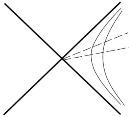
ds2 = ρ2dτ2 − dρ2− dy2− dz2. (2.15) Where ρ ≥ 0 and this Rindler coordinates (τ, ρ, x2, x3) covers only the region z ≥ |t|. It is easy to check that ρ = ρ0 describe a world line with constant proper acceleration Fig. 2.1.
It is convenient to define the coordinates (u, v) and (U, V ) u = τ − log ρ, v = τ + log ρ
U = t − x = −e−u, V = t + x = ev. (2.16) Now the metric takes the form ds2 = ρ2dudv −dy2−dz2 = dU dV −dy2−dz2. The Rindler coordinates covers V ≥ 0, U ≤ 0. The future horizon is given
Figure 2.1: Rindler Coordinates.
by U = 0, corresponds to v = v0 and u → ∞. The past horizon is given by V = 0, corresponds to v → −∞ and u = u0.
Next we solve the wave equation in the two coordinates and calculate β(˜ω, ω) explicitly. The solutions of the equation of motion can be written in the form
ϕM,ω⃗k = e−iωt−i⃗k·⃗x
√(2π)3|ω| ϕR,˜ω⃗k = e−i˜ωτ −i(k
1x+k2y)
√(2π)|˜ω| gω⃗k˜ (ρ), (2.17) for the Minkowski observers and the Rindler observers respectively. Here ω = (µ2+ ⃗k · ⃗k)12 and ˜ω is a free parameter. gω⃗k˜ (ρ) satisfies the equation:
˜
ω2+ ρ∂ρρ∂ρ− ρ2(k12+ k22+ m2)gω⃗k˜ (ρ) = 0. (2.18) Near horizon (ρ → 0) the mass term and the transverse momentum is neg- ligible, the equation behaves like {(∂ log ρ∂ )2 + ˜ω2}gω⃗k˜ (ρ) = 0. Then ϕR,˜ω⃗k is solved as
ϕR,˜ω⃗k = (e−i˜
ωu+ αe−i˜ωv)e−i(k1x+k2y)
√(2π)3|˜ω| . (2.19)
Here α is a complex number satisfies |α| = 1. Near the past horizon (V = 0 and v → ∞)
ϕR,˜ω⃗k → e
−i ˜ωu−ik1x−ik2y
√(2π)3|2˜ω| =
|12U |i2˜ωe−ik1x−ik2y
√(2π)3|2˜ω| . (2.20) Since we are considering the null surface, the normalization of the wave function is need to be specified. Here we the normalization as
i
∫ ∞
−∞
du
∫
d2⃗x(ϕ∗R,˜ω⃗k∂uϕR,˜ω′⃗k′ − ∂u(ϕ∗R,˜ω⃗k)ϕR,˜ω′⃗k′)
= i
∫ 0
−∞
dU
∫
d2⃗k(ϕ∗R,˜ω⃗k∂UϕR,˜ω′⃗k′ − ∂U(ϕ∗R,˜ω⃗k)ϕR,˜ω′⃗k′)
= δ(˜ω − ˜ω′)δ2(⃗k − ⃗k′) (2.21)
With the same normalization ϕM,ω⃗k is
ϕM,ω⃗k = e−i(ω+k
3)U2e−ik1x−ik2y
√(2π)3|¯ω| . (2.22)
Where ¯ω = ω + k3. With these preparation we can calculate β(ω, ˜ω) and obtain the expectation velues of Nω
β(ω, ˜ω) = −
∫ 0
−∞
dU ω
2π√|˜ωω||U|
i˜ωe−iωU
= −
∫ ∞
0
dτ 2π
√|ω|
|˜ω|e
2˜ωi log τeiωτ
= −
∫ ∞
0
ds 2π
1
|ω˜ω|e
2˜ωi log s+ise−2˜ωi log ω
= − 1 2πe
−˜ωπ−2˜ωi log ωΓ(1 + 2 ˜ωi) 1
|˜ωω|. (2.23) The last line can be carried out by complex path integral. Nω is given by
∫
β(˜ω, ω)β∗(˜ω′, ω)dω = e−2 ˜ωπ
∫
e−2i log ω(˜ω−˜ω′)Γ(1 + 2˜ωi)Γ(1 − 2˜ω′)
|˜ω˜ω′|
dω 4πω
= e−2˜
ωπ
2 sinh (2˜ωπ)δ(˜ω − ˜ω
′). (2.24)
Here we used equation Γ(s)Γ(1−s)1 = sin (πs)π in the last line. Now we obtain the thermal distribution Nω = 1−e14 ˜ωπ. Note that energy of the wave function ϕRω is given by ω2 (at past horizon U = T + Z = 2T ), the temperature of this thermal distribution is TR= β1
R =
1 2π.
To make the meaning of Unruh effect concrete, the Unruh detector is proposed
(a) The detector will react to states which have positive frequency with respect to the detectors proper time, not with respect to any universal time. (b) The process of detection of a field quanta by a detector, defined as the exciting of the detector by the field, may correspond to either the absorption or the emission of a field quanta when the detector is an accelerated one.
With these assumptions one can show that a uniformly detector will record finite temperature while a inertial detector record nothing. We will come back to this model in Chapter 3. As we have already seen, the es- sential reason for this result is that the detector measures frequencies with respect to its own proper time. For an accelerated observer, this definition of positive frequency is not equivalant to that of a nonaccelerated observer. In Minkowski spacetime, positive frequency defined with respect to any geodesic detectors are all equivalent. However in noneflat spacetime, two equally valid geodesic detectors may disagree on whether there are field quanta present. Hence the concept of particles is observer dependent. It is natural to ask that how can we detect the Unruh effect. I will discuss this point in Chapter 3.
2.2 Black Hole Physics
Black hole gives many implications to the microscopic structure of space- time. Here I am going to review the thermodynamics and the Hawking radiation of the black holes.
2.2.1 Black Hole Thermodynamics
Consider that a black hole swallows a hot body possessing a certain amount of entropy. Then the observer outside it finds that the total entropy in the part of the world accessible to his observation has decreased. This disappearance of entropy could be avoided in a purely formal way if we simply assigned the entropy of the ingested body to the inner region of the black hole. But this solution is unsatisfactory because the outside observer can not determine the amount of entropy absorbed by the black hole. Quite soon after the absorption, the black hole becomes stationary and completely forgets the information of the ingest body and its entropy.
If we are not inclined to forgo the law of non-decreasing entropy because a black hole has formed somewhere in the Universe, we have to conclude that any black hole by itself possesses a certain amount of entropy. A hot body falling into it not only transfers its mass, angular momentum and electric charge to the black hole, but also transfers its entropy S. As a result, the entropy of the black hole will increase when something falling to it. Beken- stein noticed that the properties of the black hole horizon area, A, resemble those of entropy. Indeed with the following correspondences
T = ~κ
2πkc, S = A
4G~, E = M c
2, (2.25)
there is an analogy between thermodynamics and black hole physics. People formulated the four laws of black hole physics, which are similar to the four laws of thermodynamics.
Zeroth law: The surface gravity of a stationary black hole is constant everywhere on the surface of the event horizon.
The zeroth law corresponds to that thermodynamics does not permit equilibrium when different parts of a system are at different temperatures. The existence of a state of thermodynamic equilibrium and temperature is postulated by the zeroth law of thermodynamics. This zeroth law of black hole physics plays a similar role. This proposition was proved under the
assumption of the energy dominance condition
TαβTγθgαγuβuγ ≥ 0, (2.26) which is that Tαβuβ is a non-spacelike vector. Where Tαβ is the energy momentum tensor and uµ is an arbitrary timelike vector field.
First law: When the system incorporating a black hole switches from one stationary state to another, its mass changes by
dM = T dS + ΩdJ + µdQ + δq, (2.27)
where dJ and dQ are the changes in the total angular momentum and electric charge of the black hole, respectively, and δq is the contribution to the change in the total mass due to the change in the stationary matter distribution outside the black hole.
The first law is known as a mass formula of the black holes. And this can be generalized to the higher derivative gravity, known as Wald formula [8]. The entropy of black hole is just the Noether charge.
Second law: In any classical process, the area of a black hole, A, and hence its entropy S, do not decrease:
∆S ≥ 0. (2.28)
The second law is known as the Hawking’s area theorem, which is proved with the weak energy condition
Tαβuαuβ ≥ 0. (2.29)
In both cases of thermodynamics and black hole physics, the second law sig- nals the irreversibility in the system. As in thermodynamics, the entropy stems from the impossibility of extracting any information about the struc- ture of the system, the structure of the black hole. Note that this second law is classical, the quantum effects can violate Hawking’s area theorem. Hawking radiation will reduce the black hole area. On the other hand, the
radiation itself is thermal and it will rise the entropy outside the black hole. So people expect the generalized second law which says that the sum of the black hole entropy and the entropy of the radiation or matter outside the black hole will not decrease. I will derive this generalized second law at chapter 4, in context of the fluctuation theorem for black hole.
Third law: It is impossible by any procedure, no matter how idealized, to reduce the black hole temperature to zero by a finite sequence of operations. The impossibility of transforming a black hole into an extremal one is closely related to the impossibility of realizing a state with M2 < a2+ Q2 in which a naked singularity would appear. Israel [9] proposed and proved the following version of the third law: A non-extremal black hole cannot become extremal at a finite advanced time in any continuous process in which the stress-energy tensor of accreated matter stays bounded and satisfies the weak energy condition in a neighborhood of the outer apparent horizon. It must be emphasized that unlike the thermodynamics, the entropy of black hole generally will not vanishes at zero temperature. The horizon area A remains finite as κ → 0.
In this section, we only reviewed the analogues between the thermody- namics and the black hole physics. The physical meanings of this black hole thermodynamics, especially for the black hole temperature will be clear in Hawking radiation.
2.2.2 Hawking Radiation
Here we consider the Schwarzschild black holes for simplicity. The essence does not change for general black holes.
The Schwarzschild black holes are described by the metric ds2 = (1 − 2M
r )dt
2− (1 − 2Mr )−1dr2− r2dΩ2. (2.30) Here M is the mass of the black hole. This metric will goes to flat at infinity, r → ∞, so (r, t) is the coordinates of the observer who stays at the infinity,
the asymptotic observer. This coordinates is singular at r = 2M , this cor- responds to the horizon of the black hole. However this singularity is just a coordinate singularity, and physical quantities will not diverge here. For example, a coordinate which is regular at the horizon can be given by
U =(2GMr − 1)12 e4GMr+t
V = −(2GMr − 1)12 e4GMr−t . (2.31) Then the metric are
ds2 = 32G
3M3
r e
−r/2GM(dU dV )− r2dΩ2, (2.32)
which is regular at r = 2M , and this coordinates correspond to coordinates of free falling observers.
Hawking radiation is related to Unruh effect via equivalence principle. Indeed, Rindler space will emerge in the near horizon limit of the black holes. For example, consider the near horizon limit (r → 2M) of the Schwarzschild metric
ds2 = (1 − 2M r )dt
2− (1 − 2Mr )−1dr2− r2dΩ2
→ (r − 2M)dt
2
2M −
2M dr2 r − 2M − r
2dΩ2
= ρ2( dt 4M)
2− dρ2− r2dΩ2. (2.33)
Here dρ = √√r−2M2M dr and ρ = 2√2M(r − 2M) > 0. The black hole horizon (r = 2M ) corresponds ρ = 0 in the Rindler coordinates.
Denote |0⟩U for Unruh vacuum which defined as the vacuum for the free falling observer, and denote |0⟩S for Schwarzschild vacuum which defined as the vacuum for the observer at spacetime infinity. Here |0⟩U corresponds to
|0⟩R and |0⟩S corresponds to |0⟩M at the previous section.
One can evaluate the Bogolubov transformation at the horizon. Then the geometry will becomes the Rindler space. Unruh vacuum is vacuum for free
falling observers near horizon, and Schwarzchild is vacuum for observers at infinity.
However the temperature TR = 2π1 obtained before is defined by Rindler time and is different from the temperature observed at infinity. One should take account the redshift from Rindler time to Schwarzchild time. For exam- ple, as we showed before (2.33), the near horizon Schwarzschild geometries can be written by:
ds2 = −ρ2( dt 4M)
2+ dρ2+ r2dΩ2. (2.34)
Where 4Mt is the Rindler time, and t is the Schwarzchild time. So the radi- ation will experience a redshift from the Rindler coordinates to the infinity observers. Hence the temperature of Hawking radiation is given by
T = 1
8πM. (2.35)
The Unruh effect just tells us that |0⟩R is different from |0⟩M, and one can find the explicit relation between |0⟩M and |0⟩. There is no problem for that which state is more natural to be vacuum. However Hawking radiation occurs for vacuum |0⟩U. If one chooses vacuum |0⟩ there will be no Hawking radiation.
There are a number of reasons why people favor the Unruh vacuum over the Schwarzchild vacuum:
(1) As we mentioned before, Unruh vacuum is the vacuum for free falling observers. It seems more natural to take the vacuum that free falling ob- server observes nothing than the vacuum that free observers boserves finite temperature.
(2) Most physical properties of the scalar field (charge density, energy, etc.) are regular for Unruh vacuum and will become singular for Schwarzchild vacuum.
(3) Unruh vacuum preserves more symmetris than Schwarzchild vacuum. For the case of flat spacetime, it is the property that |0⟩M is invariant under the full Poincar´e group while |0⟩R does not.
(4) Consider the situation that a star shell collapse to black hole, for example, the Vaidya metric, then it will turn out that Unruh vacuum is preferred.
2.2.3 Information Puzzle
The Hawking radiation from a black hole is thermal. This result is obtained in the semi-classical approximation, which is supposed to be valid until the black hole has shrunk to nearly the Planck mass. Then, if the black hole disappears completely, what is left is just thermal radiation. This also occurs even in the case when we start from some pure state collapse into a black hole. This means whatever initial state one start from, once it collapse to a black hole, the final state will be the same which is just thermal radiation. The information of the initial state are lost in this process. Or in another way to say, a pure state seems to go to a mixed state in this process. This can not happen in a quantum system with unitary time evolution. This problem is called the information loss puzzle, or information paradox.
There are many discussions on the information puzzle. However, none of them are satisfactory. The information paradox appears more like a hint or motivation than a problem, which helps people to investigate the microscopic structure of spacetime.
2.3 The Argument of Ted Jacobson
Though the black holes are just solutions of the Einstein equation, but the thermodynamics do hold for black holes. This fact is very surprisingly since the Einstein equation is just a hyperbolic second order partial differential equation. This fact may implies some connections between gravity and ther- modynamics. Some people also expects that the gravity may just be effective descriptions, like thermodynamics. Ted Jacobson [7] push this idea further.
He reversed the argument by assuming the thermodynamics of horizons first and then derived the Einstein equation.
The basic idea is following. First assume that in quantum spacetime there is a universal entropy density α per unit horizon area
S = αA, (2.36)
here A is the horizon area. Next consider the energy flux flows through this horizon as the heat, dQ. Then determine the temperature from the Unruh effect. And finally obtain the Einstein equation from the relation
δS = δQ
T . (2.37)
The local causal horizon at a point p is defined like this: choose a spacelike 2-surface patch B including p and consider the past boundary of B. Near p, this boundary is a congruence of null geodesics orthogonal to B. These comprise the horizon. Here B is chosen as such that the expansion θ and shear σab of this congruence are vanishing at p. This means the equilibrium state at p.
To define the heat flux and temperature, employ an approximate boost Killing vector field χa that vanishes at p, so its flow leaves the tangent plane Bp to B at p invariant. The direction of χa is chosen to pointing on future of the causal horizon. The normalization of χa is chosen so that χa;bχa;b = −2, just like the usual boost Killing vector x∂t+ t∂x in Minkowski spacetime. One can obtain χa by solving Killing’s equation χa;b+ χb;a = 0 in Riemann normal coordinates, yµ, order by order. However, there may be no solutions at O(y3), since a general curved spacetime may not to have a Killing vector. Killing time along the horizon is given by the parameter v such that χµ∇µv = 1. This Killing time is related to the affine parameter along the horizon generators by λ = −e−v, the point p is located at infinite Killing time and λ = 0. It will be convenient to work in terms of horizon tangent vector kµ which is related to χa by χa= −λka.
Now consider the heat as the energy current of matter across the horizon δQ =
∫
TµνMχµdΣν, (2.38)
where TµνM is the stress tensor of matter. The integral is taken over a short segment of a thin pencil of horizon generators centered on the one that ter- minates at p. The temperature is given by T = 2π~ which is the Unruh temperature of the Rindler space. Thus one have
δQ T =
2π
~
∫
TµνMkµkν(−λ)dλd2A. (2.39) The entropy change δS = αδA is given by
δA =
∫
θdλd2A, (2.40)
where θ = d(ln d2A)/λ is the expansion of the congruence of null geodesics generation the horizon. Using the Raychaudhuri equation
θ dλ = −
1 2θ
2− σµνσµν− Rµνkµkν, (2.41) one can expand θ around p where λ = 0, then
δS = α
∫ [
θ − λ( 12θ2 + σµνσµν + Rµνkµkν )]
|p
dλd2A. (2.42)
Note that all quantities in the integrand are evaluated at p. Using the as- sumption of the equilibrium, θ = σab = 0 at p
δS = α
∫
Rabkakb(−λ)dλd2A. (2.43) Now if one require that δS = δQ/T holds for all local Rindler horizons through all points p. Then the integrand of (2.39) and (2.43) should be same at every point
Rabkakb = 2π α~T
M
abkakb. (2.44)
This should hold for all null vectors ka. So Rab+ Λgab= 2π
~αT
M
ab, (2.45)
here the λ is a undetermined constant since gabkakb = 0. Finally, with the entropy density α
α = 1
4~G, (2.46)
the Einstein equation with cosmological constant is derived.
2.4 Membrane Paradigm
Another interesting issue closely related to the horizons is the Membrane Paradigm. It has been shown that observer who remains outside a black hole will see the horizon to behave according to equations that describe a fluid bubble with electrical conductivity as well as shear and bulk viscosities. The membrane paradigm is a point of view that consider a black hole as a dynamical time-like surface, the membrane. It was first proposed by Kip S. Thorn, R. H. Price and D. A. Macdonald [10]. Here I am going to review an approach given by M. K. Parikh and F. Wilczek [11].
The basic idea is like this, since (Classically) nothing can emerge from a blackhole, an observer who remains outside a blackhole cannot be affected by the dynamics inside the hole. Hence we should be able to obtain the equations of motion for external region from varying the action restricted to the external universe.
But the boundary of external region is not the boundary of spacetime. Then some surface terms will be left when we varying the action to obtain the equation of motion. So we have to add some surface terms which cancel the residual surface terms and enable us to get the complete equations of motion. Interpreting these added surface terms as sources residing on the horizon will give the picture of membrane.
Here what we actually do is just dividing the space-time into two regions (the boundary is not necessary to be horizon) and rewriting the total action as
Stotal = (Sout+ Ssurf) + (Sin− Ssurf), (2.47) requiring δSout + δSsurf = 0. Then Ssurf corresponds to sources on the boundary.
Here instead of the true horizon we consider the stretched horizon, which is a time-like surface just outside the true horizon. We parameterize it’s location by α in the way that α → 0 corresponds the limit that the stretched horizon coincides with the true horizon. Many intermediate quantities will diverge at the true horizon, α also plays the role of a regulator.
This stretched horizon has several advantages over the true horizon. Un- like the true horizon the stretched horizon is a time-like (rather than null) surface. So the metric is nondegenerate, and this enable us to write down a conventional action of the stretched horizon. We can also say that the stretched horizon is more fundamental by this sense: an external observer can make a measurement and report it at the stretched horizon which can not be done at the true horizon. By the way a one-to-one correspondence between points on the true horizon and the stretched horizon is always pos- sible.
2.4.1 The Electromagnetic Membrane
For example, we consider the electromagnetic case here. The action is given by:
S =
∫
d4x√−g(− 1 16πF
µνF
µν + JµAµ). (2.48)
Restrict the integral region to external: δSout =
∫
d4x√−g(− 1 4πF
µν∇µδAν + JνδAν)
=
∫
d4x√−g{− 1 4π∇µ(F
µνδA
ν) + δAν(∇µF
µν
4π + J
ν)}
=
∫
dS √−h 1 4πnµF
µνδA ν +
∫
d4x√−gδAν( 1 4π∇µF
µν+ Jν).
(2.49) Put the second term to zero gives the Maxwell equations: ∇µFµν = −4πJν. The first term is left because we can not set δAµ to zero at the boundary of external region. To cancel this term, adding Ssurf:
Ssurf =
∫
d3x √−hjsµAµ. (2.50) Here the equations of motion at the boundary are given by:
jsµ = 1 4πF
µνn
ν. (2.51)
From the antisymmetry of Fµν this current is parallel to the horizon (jsµnµ= 0). By component, it is given by:
js0 = − 1 4πF
0bn
b = E⊥
jsA = 1 4πF
Abn b =
1
4π(⃗n × ⃗B)
A. (2.52)
This is just the relation between the surface charge and surface current and the discontinuity of electromagnetic field at the surface. So it is natural to interpret jsµ as the electromagnetic current at the surface. One can also show that js satisfies the continuity equation by using the equations of motion,
∇µjsµ = j µ s|µ =
1 4π∇µF
µνn ν
= −Jνnν. (2.53)
This means that any charges that fall into the in-region can be regarded as remaining on the surface. We did not choose the surface to be the horizon
until now. So the results obtained here do not depend on which surface we choose.
It can be show that the membrane behaves like a conductor with certain conductivity if we choose the surface to be the horizon. We impose the regularity condition that the electromagnetic fields measured by free falling observer (FFO) should not diverge at horizon. The fiducial observer (denoted by FIDO, the observer who just remaining outside the horizon) is related to the free falling observer by some infinite Lorentz boosts (β → 1). For example, EθF IDO and BϕF IDO are given by:
EθF IDO = FF IDO0θ = γFF F O0θ − βγFF F Orθ
= γ(EθF F O− BϕF F O)
BϕF IDO = FF IDOrθ = −γβFF F O0θ + γFF F Orθ
= γ(BϕF F O − EθF F O). (2.54) We obtain relation: EθF IDO= −BϕF IDO. Similarly we can also obtain EϕF IDO= BθF IDO. In summary:
E⃗∥F IDO = ⃗n × ⃗B∥F IDO = 4π⃗js. (2.55) This is the Ohm’s law for the conductor with resistivity ρ = 4π ≈ 377Ω. Here the regularity condition is equivalent to the statement that classically all radiation in the normal direction is ingoing (a black hole acts as a perfect absorber). Indeed the Poynting flux can be calculated,
S =⃗ 1
4πE × ⃗⃗ B = −j
2
sρ⃗n. (2.56)
It is always inward. This equation also describes the Joule heating.
2.4.2 The Gravitational Membrane
In order to explore more about the membrane, we fix our convention here. We denote Ua to be the tangential vectors of the world lines of the fiducial
observers(Ua = (dτd)a, where τ is the proper time of the fiducial observer). The normal vector of the hypersurface is denoted by na. Also we choose the normal vector congruence to be along the geodesics. We can parameterize the location of the stretched horizon in the way that αUa → laand αna→ la; in other words αUaand αna are equal in the true horizon limit, and the null vector la is both normal and tangential to the horizon.
The hypersurface can be regarded as a d + 1 space-time splitting, and na is the normal vector. We can also consider the (d − 1) + 1 splitting of the hypersurface, take Ua to be the normal vector, and the d − 1 part can be regarded as the space-like section of the hypersurface. We denote the metric on the hypersurface and on the space-like section by hab and γAB.
If some vector fields lie in the hypersurface, then we can define a covariant derivative on the hypersurface, denote |a to be the d-covariant derivative (the derivative on the stretched horizon) and denote ||A to be the (d − 1)- covariant derivative (the derivative on the space-like section of the stretched horizon). The covariant derivatives are related by hcd∇cwa = w|da − Kdcwcna, where Kba = hcb∇cna is the extrinsic curvature of the stretched horizon. In summary
Ua = ( d dτ)
a, U2
= −1, lim
α→0αU
a = la (2.57)
n2 = 1, ac = na∇anc = 0, lim
α→0αn
a = la (2.58)
l2 = 0 (2.59)
hab = gab − nanb,
γba= hab + UaUb = gab − nanb+ UaUb (2.60) For wa lies in the surface hcd∇cwa= w|da − Kdcwcna
∇cwc = w|cc. (2.61)
Action
Now we turn to the gravitational membrane. First we write down the action for the membrane, second we show that this membrane behaves like a fluid
which satisfies the “Navier-Stokes equation”.
The way to obtain the action of membrane is same as the electromagnetic case. But the calculation is more complicated and for gravitational case the surface has to be the stretched horizon in order to write down the action.
The Einstein-Hilbert action is given by: S[gab] = 1
16π
∫
d4x√−gR + 1 8π
I
d3xñhK + Smatter, (2.62) the integral of the second term is only over the outer boundary of the space- time. It is necessary to obtain the Einstein equations since the Ricci scalar contains second derivatives of gab. The equations of motion well known
Rab−
1
2gabR = 8πTab. (2.63)
The surface term only comes from gabδRab
gabδRab = ∇a[∇b(δgab) − gcd∇a(δgcd)]. (2.64) Note that the normal vector na is taken to point outward, and Gauss’s the- orem gives
∫
d4x√−g(gabδRab) = −
∫
d3x√−hnagbc[∇c(δgab− ∇a(δgbc))]. (2.65) Equation nanbnc[∇c(δgab − ∇a(δgbc))] = 0 and equation gab = hab − nanb enable us to replace gbcδRbc to hbcδRbc:
∫
d4x√−g(gabδRab) = −
∫
d3x√−hnahbc[∇c(δgab− ∇a(δgbc))]. (2.66) Since the variation of membrane action takes the form δSsurf =∫ d3x√−h tsabδhab, we have to rewrite this term in order to obtain the membrane action,
∫
d4x√−g(gabδRab) =
∫
d3x√−hhbc[∇a(naδgbc) − δgbc∇a(na)
−∇c(naδgab) + δgab∇c(na)]. (2.67)
Terms involving derivative of δgab will vanish in the limit that the stretched horizon approaches the true horizon:
∫
d3x√−hhbc[∇a(naδgbc) − ∇c(naδgab)] = 0. (2.68) With Kab = hbc∇cna the variation of the external action is
δSout[gab] = 1 16π
∫
d3x√−h(Khab− Kab)δhab. (2.69) We have to integrate equation (2.69) to obtain the membrane action.
Ssurf[hab] =
∫
d3x√−h(Babhab− b) (2.70) is a solution, with source terms to be
Bab = 1 16πKab
b = −16π1 K. (2.71)
If we write the variation of the membrane action by the form δSsurf[hab] = −1
2
∫
d3x√−htsabδhab, (2.72) then the membrane stress tensor is given by
tabs = 1 8π(Kh
ab− Kab). (2.73)
Just as a surface charge produces a discontinuity in the normal component of the electric field, a surface stress tensor creates a discontinuity in the extrinsic curvature. The membrane stress tensor is consistent with the Israel junction condition:
tabs = 1 8π([K]h
ab− [K]ab), (2.74)
where [K] = K+− K−is the discontinuity of the extrinsic curvature through the surface. One can also show that tabs satisfies the continuity equation by using the equations of motion:
ts |bab = 1 8π[(Kh
ab)
|b− Kab|b]
= −Tna
= −hacTcdnd. (2.75)
The “Navier-Stokes equation”
The continuity equaiton and the fact that tabs consistent with Israel junction condition imply that stretched horizon can be considered as a fluid mem- brane. Indeed, it can be shown that membrane obeys the Navier-Stokes equation.
In the limit that the stretched horizon approaches the true horizon both αUa and αna approach la:
Uc∇cna→ 1 α2l
c∇cla=
gH
α2l
a. (2.76)
Using this fact we can write down all the components of Kba. For KUU: KabUaUb = UaUb∇anb
→ α−2Ualb∇alb = α−2UblbgH
→ α−1UaUagH = −α−1gH = −g. (2.77) For KAU:
KAU = γAaUbKab → gγAaUa = 0.
If we define the extrinsic curvature of the space-like section of stretched horizon as: kBA= γAdlB|d = 21£laγAB, then KBA is given by:
KAB = γAaKabγbB = γAaγbB∇anb
→ 1
αγ
a
AγbB∇alb =
1 αk
B
A. (2.78)
We can decompose kABinto traceless part and trace part: KAB = σAB+12γABθ. Where θ is the traceless part, correspond to shear of the membrane. And θ is the trace part, correspond to expansion of the membrane. Then we can write down all the components of tsab explicitly (K = gHα+θ here):
πA = tbsaγAaUb = 1 8π(Kh
abγ
aAUb− KAU) = 0 Σ = tbsaUbUa = −K
8π + KUU
8π = − θ 8πα tABs = 1
8πα[γ
AB(g H +1
2θ) − σ
AB]. (2.79)