Recent site activity Naoki Wakamori's Website

(1)

COMPETITION IN THE MUTUAL FUND INDUSTRY: A CASE STUDY OF S&P 500 INDEX FUNDS*

ALI˙ HORTAC¸ SU ANDCHADSYVERSON

We investigate the role that nonportfolio fund differentiation and informa-tion/search frictions play in creating two salient features of the mutual fund industry: the large number of funds and the sizable dispersion in fund fees. In a case study, we find that despite the financial homogeneity of S&P 500 index funds, this sector exhibits the fund proliferation and fee dispersion observed in the broader industry. We show how extra-portfolio mechanisms explain these fea-tures. These mechanisms also suggest an explanation for the puzzling late-1990s shift in sector assets to more expensive (and often newly entered) funds: an influx of high-information-cost novice investors.

I. INTRODUCTION

An investor seeking to hold assets in a mutual fund is a consumer with many choices: in 2001 there were 8307 U. S. mutual funds in operation. If one counts different share classes for a common portfolio as separate options available to an inves-tor, the implied total number of funds to choose from exceeds 13,000. Note in comparison that there were a total of 7600 panies listed that year on the NYSE, AMEX, and Nasdaq com-bined. A mutual fund investor’s choice set has also been growing robustly over time: while there were 834 mutual funds in opera-tion in 1980, this nearly quadrupled to 3100 by 1990, and almost tripled again by 2001.1

* Zvi Eckstein and Alan Sorensen provided thoughtful suggestions regarding earlier drafts. We also thank Judith Chevalier, Lars Hansen, Thomas Hubbard, Boyan Jovanovic, Lawrence Katz, Robert Lucas, Derek Neal, Ariel Pakes, Jonathan Reuter, three anonymous referees, and seminar participants at the University of Chicago, the Society for Economic Dynamics annual meetings, INSEAD, New York University, the Economic Research Center, the National Bureau of Economic Research Industrial Organization meetings, Harvard Uni-versity, Massachusetts Institute of Technology, the University of Chicago Gradu-ate School of Business, the University of British Columbia, Purdue University, the University of Maryland, and the Stanford Institute for Theoretical Economics. Arie Toporovsky, Chris Xu, and Yoo-Na Youm provided excellent research assis-tance. We are grateful for the financial support of the National Science Founda-tion (SES-0242031) and the John M. Olin FoundaFounda-tion. Correspondence can be addressed to either of the authors at the Department of Economics, University of Chicago, 1126 East 59th Street, Chicago, IL 60637.

1. The expansion of the choice set has accompanied a steady increase in the fraction of the population taking advantage of mutual funds. Only 6 percent of households held mutual funds in 1980. By 2001 fully 52 percent of U. S. house-holds held assets in mutual funds [Investment Company Institute 2002].

The Quarterly Journal of Economics,May 2004

403

at University of Tokyo Library on June 6, 2016

http://qje.oxfordjournals.org/

(2)

An additional, less documented feature of the mutual fund marketplace is the enormous dispersion in the fees (prices) inves-tors pay to hold assets in funds, a dispersion that persists despite competition among a large number of industry firms. These fee differences are not simply a result of variation across fund sec-tors; price dispersion within (even narrowly defined) sectors is large. Table I summarizes this within-sector dispersion. The table shows fund fee dispersion moments—the coefficient of variation, the interquartile price ratio, and the ratio of the ninetieth

per-TABLE I

PRICEDISPERSION WITHINFUNDSECTORS

Sector N

Mean price

Coefficient of variation

75th to 25th Percentile

ratio

90th to 10th Percentile

ratio

Aggressive growth 1278 191.0 0.485 2.0 3.1

Balanced growth 472 164.2 0.439 2.2 3.7

High-quality bonds 862 118.1 0.566 2.5 4.9

High-yield bonds 337 167.3 0.387 2.1 3.2

Global bonds 358 182.3 0.402 2.0 3.5

Global equities 452 228.3 0.374 1.6 2.8

Growth and income 978 158.4 0.830 2.5 5.5

Ginnie Mae 182 144.0 0.460 2.4 4.0

Gov’t securities 450 131.9 0.549 2.5 4.7

International equities 1267 225.5 0.432 1.9 3.2

Income 218 170.8 0.415 2.2 3.4

Long-term growth 1812 179.4 0.421 2.0 3.1

Tax-free money market 455 62.7 0.440 1.6 3.2

Gov’t securities money market 437 59.5 0.611 1.8 4.8

High-quality muni bond 541 137.2 0.624 2.4 4.1

Single-state muni bond 1326 150.3 0.384 1.7 3.6

Taxable money market 541 79.2 0.726 2.0 7.1

High-yield money market 62 160.4 0.408 1.7 3.3

Precious metals 35 256.1 0.399 1.6 3.3

Sector funds 511 200.8 0.364 1.8 2.9

Total return 323 178.2 0.415 1.9 3.3

Utilities 94 182.8 0.359 1.7 3.2

Retail S&P 500 index funds 82 97.1 0.677 3.1 8.2

The table shows measures of price (fee) dispersion among mutual funds in various asset classes in 2000. The fund data used to calculate these figures are from the Center for Research in Security Prices (CRSP). Roughly 95 percent of the funds in the CRSP database are matched to one of these sectors, which are categorized according to the Investment Company Data, Inc. (now Standard and Poor’s Micropal) system. We follow the CRSP convention (also common in the literature) of treating each fund share class in multiclass funds as a separate fund. Multiclass funds are those that have a common manager and portfolio, but have different pricing schemes and asset purchase and redemption rules. Prices are computed from CRSP data, and are calculated as the fund’s annual fees (both management fees and 12b-1 fees if applicable) plus one-seventh of total loads, assuming a mean holding horizon of seven years, as in Sirri and Tufano [1998]. All prices are expressed in basis points. See Data Appendix for details.

(3)

centile to the tenth percentile price—for each of 22 fund objective sectors in 2000.

As is evident in the table, the seventy-fifth percentile price fund in a sector-year cell typically has investor costs about twice those of the twenty-fifth percentile fund. The ninetieth-tenth percentile price ratios indicate between three- and sevenfold fee differences. The extrema of the distribution (not shown) can ex-hibit vast dispersion; the minimum-price aggressive growth fund, for example, imposed annualized fees of only 14 basis points (i.e., 0.14 percent of the value of an investor’s assets in the fund), whereas the highest-price fund charged a whopping 1670 basis points.2

Of course, fund portfolios can vary considerably even within narrow asset classes. Perhaps price dispersion reflects within-sector differences in demand or cost structures across fund port-folios. On the demand side, certain portfolios will outperform their sector cohorts; higher prices may just reflect investors’ will-ingness to pay for better performance. As for costs, fund manag-ers create portfolios using different securities, some of which may be more expensive to analyze or trade than others. Fund prices may reflect this fact.3_{Portfolio differentiation, too, may explain in}

2. The competitive effect of entry appears to be weak throughout the indus-try. Entry coincides with increases in both average fees and fee dispersion. We regress sectoral price (fee) dispersion moments for 1993–2001 on the logged number of sector funds, allowing for sector-specific intercepts and trends. The results, available from the authors, show that average fees in the sector actually increase significantly as the number of sector funds rises. The asset-weighted mean also increases (albeit insignificantly). Several fee dispersion moments (stan-dard deviation, coefficient of variation, interquartile range, and the ninetieth/ tenth and ninety-fifth/fifth percentile fee ranges) are positively correlated with increases in the number of sector funds as well.

3. To check the price-dispersion/performance-dispersion hypothesis, we re-gress gross annual returns, the within-year average gross monthly return, and the within-year standard deviation of monthly returns on fund prices. The sample consists of all mutual funds in the CRSP database between 1993 and 2001 with return data available—roughly 83,300 fund-year observations. The specifications include interacted Strategic Insight objective category (of which there are 193) and year effects, so estimated coefficients reflect the correlation between returns and prices within sector-year cells. The price coefficients in both gross return regressions are actually negative (though statistically insignificant); more expen-sive funds have lower-than-average returns. (A regression of net annual returns on price yields a significantly negative coefficient; one would expect zero in a perfectly competitive market where price differences are exactly compensated by gross returns.) Furthermore, the correlation between fund prices and return variance is positive and significant—also the opposite sign one would expect if performance and price were closely linked. A more careful investigation would obtain measures of expected returns and use longer performance histories to measure within-fund return variation; however, given the magnitude of the ob-served price dispersion, these results suggest that the price-performance link is not an overwhelming determinant of the observed patterns in the data. The findings are also in line with Carhart [1997], where the impact of expenses on

(4)

part the large number of industry funds. Investors differ in their ideal portfolios and their current asset compositions. Perhaps thou-sands of funds and several hundred new funds each year are nec-essary to provide the many risk-return profiles sought by investors.4

However, a look at the retail (i.e., noninstitutional) S&P 500 index fund sector strongly suggests that the composition and financial performance of funds’ portfolios are not the only factors explaining fund proliferation and fee dispersion. All funds in this $164 billion (in 2000) sector explicitly seek to mimic the same performance profile, that of the S&P 500 index. Thus, any discrep-ancies among these funds’ financial characteristics should be mini-mal, and the observed competitive structures of the sector (including the important fund proliferation and price dispersion issues dis-cussed above) are likely to be driven by nonportfolio effects.

It is readily apparent that, despite the sector’s financial homogeneity, the features of the broader mutual fund industry are equally prominent. There were 85 retail S&P 500 index funds operating in 2000, a number that seems well beyond the satura-tion point arising from simple portfolio choice motives, given that each one offered conceivably equivalent expected risk-return pro-files. Entry has been brisk too: the number of funds in the sector has more than quintupled since 1992. As for price dispersion, the highest-price S&P 500 index fund in 2000 imposed annualized investor fees nearly 30 times as great as those of the lowest-cost fund: 268 versus 9.5 basis points. Table I shows that this striking divergence is not restricted to the far ends of the distribution; the seventy-fifth/twenty-fifth and ninetieth/tenth percentile price ra-tios are 3.1 and 8.2, respectively, which are both at the high end of the range among broader sectors. Even more interestingly, high-price funds are not all trivially small. The highest-fee fund held 1.1 percent of sector assets— enough to make it the tenth-largest fund in the sector and not much smaller than the 1.4 percent share of the lowest-price fund.5

This paper addresses the following puzzle: how can so many firms, charging such diffuse prices, operate in a sector where

performance was negative and at least one-for-one. Detailed results are available from the authors upon request.

4. See Mamaysky and Spiegel [2001] for an argument along these lines. 5. The sizable price dispersion is not driven simply by loads; considerable spreads are observed among annual fees (the sum of management and 12b-1 fees) alone. The comparable dispersion measures for these fees are as follows: seventy-fifth-twenty-fifth percentile price ratio⫽2.1; ninetieth-tenth percentile ratio⫽ 6.0; and max-min ratio⫽20.8.

(5)

funds are financially homogeneous? We deepen the puzzle in Section II by discussing observed price heterogeneity and entry patterns among S&P 500 index funds. Section III discusses and provides empirical evidence for the existence of several factors that may explain the observed price dispersion. We provide in Section IV a model of competition in this industry that explicitly incorporates the two factors we deem to be the most important: investors’ tastes for product attributes other than portfolio com-position, and informational (or search) frictions that deter inves-tors from finding the fund offering highest utility (net of manage-ment fees). Section V uses equilibrium conditions of our model to evaluate the ability of search and nonportfolio differentiation to qualitatively and quantitatively explain patterns in the data. In Section VI we use estimated parameters of our model to quantify the social welfare implications of having so many funds delivering what are arguably ex ante identical returns.

Estimation of our model yields the following results: product differentiation plays an important role in this “seemingly” homo-geneous product industry. Investors appear to value funds’ ob-servable nonportfolio attributes, such as fund age, the total num-ber of funds in the same fund family, and tax exposure, in largely expected ways. Our estimates also indicate that after accounting for (vertical) product differentiation across index funds, fairly small search costs can rationalize the fact that the index fund offering the highest utility does not capture the whole market. Perhaps more interestingly, our estimates imply that the distri-bution of search costs across investors that sustains observed prices and market shares has been shifting over time. While search costs were falling in the lower three quartiles of the distribution throughout our observation period (the late 1990s), costs at the high end of the distribution were rising. We show evidence suggesting that this may be due to a compositional shift in demand: the documented influx of novice (and high-informa-tion-cost) mutual fund investors during the period, whose pur-chases may underlie the observed shift in sector assets to more expensive and often newly entered funds. Given our estimates of demand parameters, our welfare calculations indicate that re-stricting sector entry to a single fund might yield nontrivial gains from reduced search costs and productivity gains from returns to scale, but these gains may be counterbalanced by losses from monopoly market power and reduced product variety.

We see the broader contribution of this paper as twofold. The mutual fund literature is not typically concerned with strategic

(6)

interactions among firms in this important industry.6 _Yet

com-petitive forces are an important determinant of the fortunes of funds and fund families as well as consumer welfare. We seek to partially fill this research gap by providing a model of competition in this industry and taking this model to data to quantify the economic forces at work.7_{The second contribution of the paper is}

methodological: the modeling and estimation framework devel-oped here can be applied to other industries where search fric-tions coexist with product differentiation. Unlike previous empiri-cal applications of models of search equilibrium (mostly in labor economics), we do not have data on individuals’ decisions and must draw inferences regarding search behavior from aggregate price and quantity data.8 _{Our methodology is closest in this}

respect to Hong and Shum [2001], who discuss identification and estimation of equilibrium search models using only market-level price data from markets for homogeneous goods. Our model ex-tends their results by showing how aggregate price and quantity data can be used to identify and estimate search costs separately from sources of vertical product differentiation, with particular attention to minimizing the impact of functional form restrictions.

II. ANOVERVIEW OF THERETAIL S&P 500 INDEXFUNDSSECTOR

S&P 500 index funds are the most popular type of index mutual funds. Their explicit investment objective is to replicate the return patterns of the S&P 500 index. Many do so by holding equities in the same proportions as their index weights, while

6. This literature, too vast to cite comprehensively, follows from the classic contributions on portfolio theory and empirical testing as well as the principal-agent framework. See, for example, Jensen [1968], Malkiel [1995], Falkenstein [1996], Gruber [1996], and Chevalier and Ellison [1997, 1999].

7. We should note that there has been a recent increase of interest among financial economists in this area. For example, Sirri and Tufano [1998] note that mutual fund flows are relatively insensitive to management fees and excessively sensitive to past performance (as opposed to expected performance). Khorana and Servaes [1999, 2003] empirically explore what market characteristics are corre-lated with fund entry and the market share of fund families. Barber, Odean, and Zheng [2002] find that fund inflows seem to be more responsive to some price instruments than others, and that advertising appears to be an effective tool for increasing fund assets. On the theoretical side, Massa [2000] and Mamaysky and Spiegel [2001] explore the driving forces of fund creation.

8. Sorensen [2001] is a recent attempt in the industrial organization litera-ture to estimate search costs using consumer-level product choice data. Examples of structural estimation of search models in labor markets include Flinn and Heckman [1982], Eckstein and Wolpin [1990], and van den Berg and Ridder [1998].

(7)

some use other index-matching methods like statistical sampling and index derivatives.

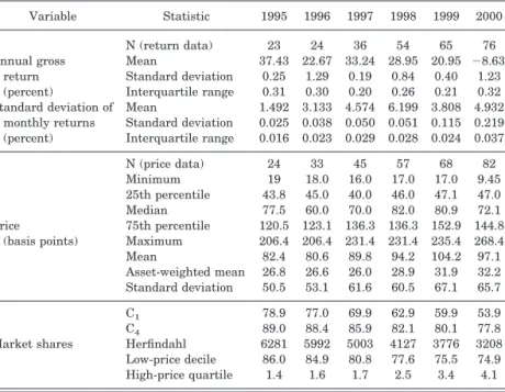
Despite the existence of different index replication strategies, there is considerable financial performance homogeneity in our sample of S&P 500 index funds.9_{The top rows of Table II contain}

summary statistics of our sample funds’ gross annual returns and

9. We exclude institutional S&P 500 funds from our sample, despite the fact that they also mimic the same performance profile, because we believe they operate in a fundamentally different product market than noninstitutional funds (more on this below). By doing so, we hope to further control for unobservable differences across funds that might confound our analysis. We also exclude “en-hanced” index funds, which blend active trading strategies with passive index-holding.

TABLE II

EVOLUTION OFRETAILS&P 500 INDEXFUNDSECTOR

Variable Statistic 1995 1996 1997 1998 1999 2000

N (return data) 23 24 36 54 65 76

Annual gross Mean 37.43 22.67 33.24 28.95 20.95 ⫺8.63 return Standard deviation 0.25 1.29 0.19 0.84 0.40 1.23 (percent) Interquartile range 0.31 0.30 0.20 0.26 0.21 0.32 Standard deviation of Mean 1.492 3.133 4.574 6.199 3.808 4.932

monthly returns Standard deviation 0.025 0.038 0.050 0.051 0.115 0.219 (percent) Interquartile range 0.016 0.023 0.029 0.028 0.024 0.037

N (price data) 24 33 45 57 68 82

Minimum 19 18.0 16.0 17.0 17.0 9.45

25th percentile 43.8 45.0 40.0 46.0 47.1 47.0

Median 77.5 60.0 70.0 82.0 80.9 72.1

Price 75th percentile 120.5 123.1 136.3 136.3 152.9 144.8 (basis points) Maximum 206.4 206.4 231.4 231.4 235.4 268.4

Mean 82.4 80.6 89.8 94.2 104.2 97.1

Asset-weighted mean 26.8 26.6 26.0 28.9 31.9 32.2 Standard deviation 50.5 53.1 61.6 60.5 67.1 65.7

C1 78.9 77.0 69.9 62.9 59.9 53.9

C4 89.0 88.4 85.9 82.1 80.1 77.8

Market shares Herfindahl 6281 5992 5003 4127 3776 3208 Low-price decile 86.0 84.9 80.8 77.6 75.5 74.9 High-price quartile 1.4 1.6 1.7 2.5 3.4 4.1

The table shows characteristics of our retail (i.e., noninstitutional) S&P 500 index funds sample. As in Table I, we treat each fund share class in multiclass funds as a separate fund. (If we were to count multiple-class funds as single funds, there would be 50 funds in 2000.) We also include exchange-traded funds (ETFs) based on the S&P 500 index. There is only one ETF for most of our sample, Standard & Poor’s Depositary Receipts (SPDRs). In 2000 a second ETF, Barclay’s iShares S&P 500 Index Fund, started trading. We report price figures for only 82 funds in 2000 because we lack price information for three funds. Reported returns data are limited to funds reporting returns in every month of a given year to avoid comparing figures

from funds operating in nonrepresentative portions of the year. C1(C4) is the fraction of sector assets in the

largest (largest four) funds. The Herfindahl index is the sum of the squared market shares (expressed as percentages). Low-price decile and high-price quartiles are the combined market shares of the lowest-price and highest-price fund quantiles, respectively.

(8)

standard deviations of their monthly gross returns. As can be seen, the relative dispersion in return patterns is quite small. The interquartile range of gross annual returns is no greater than 0.32 percentage points, and is typically about 1 percent of the mean.10 _{The dispersion of the standard deviation of funds’}

monthly returns is similarly slight: the average interquartile range-mean ratio is 0.007, and the coefficient of variation is under 5 percent in every year. These small variations suggest that investors would be justified in presuming common ex ante re-turns among our funds.11

Despite this homogeneity in financial performance, the sector shares the fund proliferation and price dispersion traits seen in the broader mutual fund industry. There was vigorous growth in both the number of retail S&P 500 index funds and their total net assets under management from 1995 to 2000, our period of ob-servation. This was coincident with and even stronger than the overall growth in the mutual fund industry documented above. The number of sector funds more than tripled from 1995 to 2000 (from 24 to 85), and sector assets grew at twice the rate as did total equity fund assets.12

Figure I and the middle portion of Table II show the evolu-tion of the sector’s price distribuevolu-tion over our sample period. A striking feature of Figure I, which plots the cumulative price distribution functions of sector funds, is the rightward shift in the price distribution from 1996 to 1999. (This trend interestingly reversed in 2000.) The movement was steady; the 1997 and 1998

10. Statistics on returns in the table correspond only to funds operating every month in observed year to eliminate composition bias from funds with return data spanning only a possibly nonrepresentative portion of the year. While the disper-sion patterns are largely mirrored in the standard deviations of the return moments, outliers do enlarge the standard deviation of annual returns in some years, to as much as 14 percent of the mean in 2000. An index fund’s performance can deviate from the index which it is tracking (and from other funds tracking the same index) because of several factors. These include idiosyncratic portfolio sales required to meet the particular daily activity needs of a fund, how much of the fund’s assets are held in cash, and the timing of trades.

11. As with the broader sample discussed above, a regression using our S&P 500 funds indicates a significantly negative correlation between net annual re-turns and price, suggesting that higher prices are not being compensated by higher gross returns of equal size. Also, as with the broader sample, a regression of the standard deviation of funds’ monthly returns on price indicates a positive and significant correlation. This is of course the opposite sign predicted by a close price-performance link. (Year fixed effects are included in both regressions.)

12. Sector growth was driven in part by the growing popularity of passive management strategies among investors. The S&P 500 index fund sector was particularly able to capitalize on this preference shift partly because the original index fund, the First Index Investment Trust, is today the Vanguard 500 Index Fund. Its early entry into a growing sector has been seemingly very important: the Vanguard 500 Index Fund still is a dominant player in the sector.

(9)

distributions mark continuities in the evolution. The shift oc-curred throughout the distribution, but particularly at the high end. As can be seen in Table II, this shift happened despite the entry of nearly a dozen funds a year and a steady drop in con-centration during the period. Along with the increase in average price evident in the figure, the table also documents an increase in price dispersion: the interquartile range and standard devia-tion of prices increase (though not monotonically) over the obser-vation period.

An interesting related observation is the change in the rela-tive market shares of the high- and low-price segments. It is evident in the bottom of Table II that while low price funds still dominate the market, the asset share of funds in the lowest price

FIGUREI

Price Cumulative Distribution Functions

The figure shows, by year, c.d.f.s of the retail S&P 500 index fund price (fee) distributions. Prices are computed from Center for Research on Security Prices (CRSP) data, and are calculated as the fund’s annual fees plus one-seventh of total loads. All prices are expressed in basis points. See Data Appendix for details.

(10)

decile has fallen consistently since 1995. In contrast, the market shares of the upper quartile (and decile, not shown) rose during the same period. The proportional rise in sector assets held in expensive funds has been especially stark; the market share of the top quartile nearly tripled. The reallocation of market share to higher-priced funds resulted in a 20 percent rise in the sector’s asset-weighted average price from 1995 to 2000, from 26.8 to 32.2 basis points. Indeed, if the asset-weighted mean price had held constant at 1995 levels, total annualized fees would have been $88.5 million lower in 2000.

Recall that these increases in price dispersion and levels are occurring in concert with robust entry into the sector. An exami-nation of entry patterns sheds additional light on this issue. From 1995 through 1999, while 25 funds entered the sector with prices above 100 basis points, only seven funds charging less than 40 basis points entered. Using the decomposition method of Foster, Haltiwanger, and Krizan [2002], we found that the entrants’ asset-weighted average price was higher than the weighted mean among incumbents in each year from 1995 to 1999. Moreover, entry was the predominant contributory factor in the two years with the largest average share-weighted price increases (1998 and 1999).13

III. SOURCES OFPRICEDISPERSION

We have documented above that portfolio differentiation is an unlikely explanation of the observed price dispersion and entry/asset-reallocation patterns. In this section we discuss and provide empirical evidence for and against three mechanisms that might explain these seeming anomalies: nonportfolio “prod-uct” differentiation of mutual funds, search costs/information frictions, and switching costs. This discussion will motivate our model of industry equilibrium and its detailed empirical investi-gation in Sections IV, V, and VI.

III.A. Nonportfolio Differentiation

Fund attributes other than portfolio composition are one possible reason investors would value funds differently. If port-folio returns come bundled with a set of services that differ across

13. See Table 4 of Hortac¸su and Syverson [2003], which breaks changes in the (asset-based) market-share-weighted mean price into within, between, and net entry components (also see Hortac¸su and Syverson, footnote 16).

(11)

funds, price dispersion among financially homogeneous funds could be sustained. Capon, Fitzsimmons, and Prince [1996] report from a survey administered to roughly 3400 mutual fund holders that investors consider the number of other funds in the family and the fund company’s responsiveness to enquiries as the third-and fourth-most important criteria (respectively, after perfor-mance and manager reputation) in their mutual fund purchase decision. These fund attributes are not directly related to the financial characteristics of a fund’s portfolio, and could well ac-count for price differences across funds with equivalent return profiles.

Other such attributes might play a similar role. For example, the provision of financial advice, usually bundled with the pur-chase of load funds, is important to many investors: 60 percent reported consulting a financial adviser before purchase [Invest-ment Company Institute 1997]. We explore this influence in de-tail below. Other potentially important attributes explored below are whether the fund is an exchange-traded fund, its age, the tenure of its manager, its rate of taxable distributions, and the quality of its account services (frequency and quality of account statements, account access by phone, etc.).

We incorporate such nonportfolio differentiation into our model in Section IV. Funds differ in their offered utility levels because they have varying amounts of attributes valued by in-vestors. We assume that all investors place the same values on these qualities. It seems possible, though, that horizontal taste differences (like differing tastes for certain attributes or a logit-type random utility term) may exist in conjunction with the modeled vertical component. We have explored more general preference specifications that incorporate both horizontal taste differences and search cost variation across consumers. However, as will be seen below, market outcomes driven by horizontal differentiation cannot in general be separately identified in our data from those caused by search costs. This unfortunately pre-vents us from estimating such models and directly testing for horizontal taste variation. We do, however, estimate a specifica-tion that allows a particular form of horizontal differentiaspecifica-tion where investors differ by type in terms of whether they buy a fund through an intermediary bundling advisory services for a load (sales charge), or through “direct” channels that lead to no-load fund purchases. As will be discussed, this specification reflects the institutional setup of the industry well, and provides inter-esting insights into structural changes in demand.

(12)

III.B. Search Costs/Information Frictions

An additional (but not mutually exclusive from product dif-ferentiation) possible explanation for the observed price disper-sion is the influence of search/information frictions faced by in-vestors. A large theoretical literature shows that costly search can sustain price dispersion in homogeneous product markets (e.g., Burdett and Judd [1983], Carlson and McAfee [1983], and Stahl [1989]). Given the very large number of mutual funds offered, it seems reasonable to presume that investors must make some information-gathering investments before deciding between fund alternatives. The presence of a sizable market to reduce investor search costs supports this notion. Several commercial mutual fund ranking services and information aggregators exist (Morningstar, Lipper, Valueline, Yahoo!Finance, etc.). There is even a commercial Internet site (IndexFunds.com) devoted to providing information about index funds. Many fund companies spend considerable sums on marketing and distribution, also consistent with (although neither necessary nor sufficient for) the presence of limited investor information. Survey evidence also suggests considerable information-gathering. The Investment Company Institute [1997] reports that surveyed investors con-sulted a median of two source types (four for those who had consulted a fund-ranking service) and reviewed a median of four-teen different information items (gross returns, relative perfor-mance, etc.) before their most recent purchase.14_{To the extent}

that gathering and analyzing such information consumes inves-tor time and money, these activities constitute costly search.

Aside from this anecdotal evidence, price patterns among institutional-class S&P 500 index funds offer more direct sub-stantiation of the importance of search frictions in the sector. As mentioned before, we do not include these institutional funds in our analysis because of our belief that they operate in a funda-mentally different product market. The very high initial mini-mum investment levels (typically at least $1 million) restrict demand to a fairly narrow class of investors. It also implies that if there is investor search, there is a larger gain (in absolute levels) to finding a lower-price or higher-quality fund for a typical institutional buyer than for a retail investor. It might then be

14. The survey was administered at the very beginning of Internet access diffusion among the general public. The use of online sources has surely risen since then, raising the possibility that per-fund search costs have declined since the beginning of our sample period. We address this issue in more depth below.

(13)

reasonable to assume that there are higher search intensities among institutional funds, implying less price dispersion and lower average prices. The data are consistent with this. Figure II compares histograms of institutional and retail fund prices in 2000. It is readily apparent that the former distribution is con-siderably tighter and has a smaller mean. While administrative cost advantages may be in part responsible for the lower average price of institutional funds, they are unlikely to affect price dis-persion. We cannot rule out all other explanations for these dif-ferences, but this prima facie evidence is suggestive of search.15

III.C. Switching Costs

An additional explanation for some of the patterns docu-mented above are the switching costs involved when investors move assets across fund families (intrafamily transfers are typi-cally free). These costs could either be “formal” (like those created by deferred or rear loads) or “informal” (the hassle associated with drafting a letter to the fund company to approve withdraw-als, for example). While in many ways similar to search costs, switching costs are distinct. With search, an investor considering moving assets to another family knows the utility benefit from staying but must pay a cost to learn the benefit of going else-where. Switching costs, on the other hand, imply that the investor knows the utility benefit of moving her money to another fund company, but a cost must be paid to move. To separately identify these two factors, we would need to exploit variation in investors’ information sets. Unfortunately, this decomposition is very diffi-cult if not impossible without detailed investor-level data, so we cannot directly test a “search versus switching costs” hypothesis in our model.

Still, some information is available that allows us to obtain a general idea of the size of switching cost effects, and we attempt to do so here. Informal switching costs are difficult to quantify, but the mechanism by which formal switching costs like rear and deferred loads operate is obvious: investors with

rear/deferred-15. In particular, this evidence (as well as some of the other patterns de-scribed above, perhaps) is also consistent with Gabaix and Laibson’s [2003] intriguing suggestion that mutual fund companies “confuse” boundedly rational investors by giving them noisy signals about the surplus from their fund pur-chase— e.g., by utilizing complicated nonlinear pricing schemes. They show that such endogenously supplied “confusion” enables price dispersion to be sustained among homogeneous products and results in entry leading to price increases. Our evidence is consistent with their explanation in that institutional investors are likely to be less bounded in their rationality and hence more difficult to “confuse” than retail investors—sustaining lower levels of price dispersion.

(14)

FIGUREII

2000 Price Histograms, Retail and Institutional Funds

The figure shows the price histograms for retail and institutional S&P 500 index funds in 2000. Prices are calculated as annual fees plus one-seventh of total loads. All prices are expressed in basis points.

QUARTERLY

JOURNAL

OF

ECONOMICS

(15)

load fund holdings must pay a charge (typically up to 5 percent) if they remove those assets from the family within a specified time period. For such investors, this gives the S&P 500 index fund run by the load fund family an advantage over (often lower-priced) S&P 500 index funds offered by others.16 _{In particular,}

such load-driven switching costs may lead to “parking” behavior, where investors holding non-S&P 500 index funds in the family move assets over to (or “park” in) the family’s S&P 500 fund when dissatisfied with the performance of the other (possibly actively managed) funds in the family. Given that several fund families specializing mostly in actively managed funds opened an S&P 500 index fund in this period, one might conjecture that the market share gains made by these entrants (typically high-priced, as we have shown) is driven in part by the captive demand of “parkers.”

To gauge the empirical importance of such behavior, we search for patterns that one might expect to see in our data if switching-cost-induced parking behavior is important. One pat-tern regards the response of asset flows into our S&P 500 index funds to the relative performance of other funds within the same fund family. It seems likely that the overall performance of a family’s funds influences flows into or out of specific funds within the family, say through “star” fund effects or similar perfor-mance-spillover mechanisms. If such a performance spillover ex-ists, high (low) average performance of a fund family’s non-S&P 500 funds should, all else being equal, boost (decrease) net asset inflows into the family’s S&P 500 fund. However, this spillover into the S&P 500 fund should be damped in load fund families if switching-cost driven parking is important: when a load fund family’s non-S&P 500 funds experience a period of low (high) performance, the parking response will cause investors holding assets in the family’s other funds to move money into (out of) the family’s S&P fund. This movement would counteract in part the spillover-driven flows.

To test this hypothesis, we regress annual net dollar flows into our S&P 500 index funds on an asset-weighted average performance measure of the non-S&P 500 index funds in the

16. Front loads, while sunk, still create switching costs through a more subtle mechanism. If front-load fund owners remove assets from the family, they lose the option value of being able to transfer those assets among that family’s funds without paying additional loads. Once the assets are moved out, another load must be paid if they should choose to bring them back in. (We thank a referee for pointing out to us this option value.)

(16)

same family. The performance measure we use for the non-index funds is the weighted mean of the Sharpe ratio of these funds’ excess returns relative to the S&P 500 fund (or a weighted aver-age among the index funds if there is more than one in a family). After including year dummies and fund fixed effects in our re-gressions, we find a positive and significant correlation between flows into the S&P 500 fund and the performance of the non-S&P 500 funds in the family. This finding is consistent with our pre-sumption that performance spillovers exist. However, when we allow the magnitude of the response of S&P 500 index fund flows to the performance of other funds in the family to differ between load fund families and no-load fund families, we do not find a statistically significant difference. This goes against the hypothe-sis that switching costs in load fund families damp the spillover-induced net flows to their S&P 500 index funds.

A second empirical pattern one may expect to observe if switching costs and parking behavior are important is that with-in-familyasset share of S&P 500 index funds should grow faster in load fund families than in no-load families. Sector growth over our observation period led to virtually all S&P 500 funds com-prising larger shares of their family’s overall assets over time. If switching costs are important, the introduction of a new S&P 500 index fund in a load fund family may induce captive within-family investors to switch into this new offering, in addition to any new investors arriving at the fund family. This suggests that the within-family asset share of S&P 500 index funds in load fund families may grow faster than their counterparts in no-load fam-ilies, as fund holders in load families take advantage of their newfound ability to park their assets in the index fund.

We do not find evidence of this second pattern in our data. We regress (at the fund family level) the change in the within-family asset share of their S&P 500 index funds on a set of year dummies and an indicator for load families. The estimated coefficient on this latter dummy is negative and insignificant. A similar regres-sion was run with the growth rate of the within-family share (rather than just the share change) as the dependent variable. Here the load-family dummy was positive and insignificant. Hence, rather than the faster growth in load fund families im-plied by high switching costs, it seems that there is no appreciable difference across load and no-load families in the growth of with-in-family asset shares of S&P 500 index funds.

While we do not interpret the outcomes of these simple tests as evidence thatnoload-driven switching costs exist in the sector,

(17)

they do suggest to us that their effects might not be as large as one may think. We also note that the concept of a typical investor locked into holding assets in a single fund family due to switching costs is inaccurate: for example, the Investment Company Insti-tute [2000] reports the median number of mutual fund companies with which investors hold assets is two.

Given this evidence, the theoretical model we will develop in the next section will not include switching costs as an explicit component. Still, we believe that switching costs created by the fund family structure of the industry play some role in the S&P 500 index fund sector. We attempt to account for this influence in our empirical model—albeit in an imperfect manner— by letting investors’ purchase decisions depend on the size of funds’ man-agement companies, and by allowing investors to respond to the presence of a rear/deferred load independently from the presence of bundled advice. Furthermore, given the conceptual similarity between switching and search costs discussed above, we expect that some switching cost effects are likely to be reflected in our estimates, suggesting a broader interpretation of our estimates of “investor search costs” beyond information-gathering costs alone.

IV. THEMODEL

IV.A. General Setup

Demand for sector funds is characterized by a continuum of investors searching over funds with varying attributes.17

Inves-tors have heterogeneous search costs, and we also allow for the fact that some index funds are “easier to find” than others by allowing heterogeneous sampling probabilities across funds. We assume that fund attributes are vertical characteristics, and that all investors share a common utility function. Thus, conditional on investing in fundj, an investor receives indirect utility equal touj(Wj;␪), whereWjis a vector of fund attributes and␪is a set

of parameters that characterize how the attributes affect utility. The model requires few specific assumptions on the form ofuj⵺a

priori. However, for reasons that will become clear in the next section, we assume utility is a linear function of fund characteristics:

(1) uj⫽Wគj␤⫺pj⫹␰j,

17. See Anderson and Renault [1999] for an alternative model with costly search over differentiated products.

(18)

where Wគj are the elements of Wj other than price pj and an

unobservable component␰j. Note that the coefficient on the price

term has been normalized to ⫺1, so utilities are expressed in terms of the unit of price measurement. Here, given the nature of the good, that unit is basis points. Thus, one can think ofuj as

specifying fund utility per dollar of assets the investor holds in it. Despite a clear rank ordering of funds, the fund delivering the largest uj does not gain 100 percent market share because

search is costly. We assume that search costs are heterogeneous in the investor population and have distributionG(c). Investors incur this cost to learn the indirect utility of a particular fund, with the exception of the first fund they search (this assures all investors desiring to hold assets in the sector end up doing so regardless of their search cost level). For tractability we assume that investors search with replacement and are allowed to “re-visit” previously searched funds. We also restrict investors to purchase shares in only one S&P 500 index fund.18

Define investors’ belief about the distribution of funds’ indi-rect utilitiesH(u). Then the optimal search rule for an investor with search costci is to search for another fund as long as

(2) ciⱕ

冕

u* u៮

共u_⫺u*兲 dH共u兲,

whereu៮ is the upper bound ofH(u), andu* is the indirect utility of the highest-utility fund searched to that point. This is a stan-dard condition in sequential search models; search continues if the marginal cost of search is no greater than the expected mar-ginal benefit. We simplify matters by assuming that investors observe the empirical cumulative distribution function of funds’ utilities. That is, label the N funds by ascending indirect utility order,u₁ ⬍ . . .⬍ uN. Then, under equal sampling probabilities

(an assumption we will relax momentarily),

(3) H共u兲⫽_N1

冘

j⫽1 N

I关ujⱕu兴.

18. Following Carlson and McAfee [1983], the search-with-replacement as-sumption greatly simplifies matters in search models involving a finite number (as opposed to a continuum) of products because we do not need to worry about how investors’ beliefs about the price distribution evolve as certain funds are removed from consideration. This deviation from reality is small when there are a large number of funds. The revisit assumption implies of course that the investor’s benefit from searching is relative to the best fund yet searched, rather than the particular fund in hand at any given time.

(19)

Thus, investors know the available array of indirect utilities; they just do not know which fund provides what utility level until engaging in costly search.

The optimal search rule yields critical cutoff points in the search distribution, given by

(4) cj⫽

冘

k⫽j N

␳k共uk⫺uj兲,

where␳kis the probability that fundk is sampled on each search

(these probabilities are known by investors), andcjis the lowest

possible search cost of any investor who purchases fund j in equilibrium. The intuition behind this expression is as follows. Optimal search continues until the investor’s expected benefit from searching is lower than the search cost. The right-hand side of expression (4) is the expected benefit of additional search for an investor who has already found fundj. This is the product of the probability ␳k that another search yields a higher-utility fund

(recall that uk ⬎ ujifk ⬎ j) and the corresponding utility gain uk ⫺ uj, summed over all funds superior to fundj. Fund draws

with utilities less than uj are ignored in this calculation, as

investors can costlessly revisit funds already searched. Note that this expected benefit declines in the fund’s index; in fact,c_N⫽0. Thus, as long as an investor’s search cost is lower thancj, he or

she keeps searching until a fund offering greater utility than fund

j is found. On the other hand, more search is not worthwhile for any investor with search costs greater than cj who finds fundj.

Notice that this implies the product index is declining in the ordinal ranking of critical search cost values; i.e., whileu1⬍ . . . ⬍ uN, cN ⬍ . . . ⬍ c1.

We can use this optimal search behavior to identify elements of the search cost distribution. Funds’ market shares can be written in terms of the search cost c.d.f. by using the search-cost cutoffs above. Consider the lowest-utility fundu1. This fund has

a high cutoff search valuec1, because any investor having already

found this fund has a large expected benefit from continuing to search. Therefore, only investors with very high search costs (c⬎

c₁) purchase the fund. At the same time, though, notallinvestors withc⬎c1purchase the fund, only those (unfortunate ones) who

happen to draw fund 1 first—which happens with probability␳1.

Thus, the market share of the lowest-utility fund is

(20)

(5) q1⫽␳1共1⫺G共c1兲兲⫽␳1

冉

1⫺G

冉

冘

k⫽1 N

␳k共uk⫺u1兲

冊冊

.

Now consider the market share of the second-lowest utility fund, fund 2. Again a fraction of the highest-search-cost investors (c ⬎ c1), unable to afford a second search, find fund 2 first and

purchase it. But a subset of investors with search costsc1⬍ c⬍

c2 also purchase fund 2; namely, those who find fund 2 on their

first search, or those search only to find fund 1 and keep searching until they draw fund 2. This happens with probability ␳2/(1 ⫺ ␳1).19Thus, the total market share of fund 2 is

(6) q2⫽␳2共1⫺G共c1兲兲⫹ ␳2

1_⫺␳1关G共c1兲⫺G共c2兲兴

⫽␳2

冋

1_⫹␳1G共c1兲 1_⫺␳1 ⫺

G共c2兲

1_⫺␳1

册

.

Analogous calculations, detailed in the Appendix, produce a gen-eralized market share equation for funds 3 throughN:

(7) qj⫽␳j

冋

1⫹

␳1G共c1兲

1_⫺␳1 ⫹

␳2G共c2兲共1_⫺␳1兲共1_⫺␳1⫺␳2兲

⫹

冘

k⫽3 j⫺1

␳kG共ck兲

共1_⫺␳1⫺. . . ⫺␳k⫺1兲共1⫺␳1⫺. . . ⫺␳k兲

⫺_共₁ G共cj兲

⫺␳1⫺. . . ⫺␳j⫺1兲

册

. These equations form a system of linear equations linking

G(c₁), . . . ,G(c_N_⫺₁)—the population fractions with search costs less than the distribution’s critical values—to observed market shares. Moreover, we know that G(c_N) ⫽ 0 because (4) implies that c_N ⫽ 0 and search costs cannot be negative.20

The market supply side is comprised of funds that choose prices to maximize current profits. Let S be the total size of the

19. The total probability that a search sequence yields only fund 1 draws until a fund 2 draw is␳1␳2⫹ ␳1␳1␳2⫹ ␳1␳1␳1␳2⫹. . .⫽ ␳1␳2/(1⫺ ␳1). Summing with

the probability that the first draw is fund 2 (␳₂) yields␳2/(1⫺ ␳1).

20. Notice that since G(cN)⫽ 0, the market share equations only include

N⫺1 values ofG(c).

(21)

market,pjandmcjbe the price and (constant) marginal costs for

fund j, andqj be the fund j’s market share given the price and

characteristics of all sector funds. Then the profits of fundjare (8) ⌸k⫽Sqj共p, Wគ兲共pj⫺mcj兲.

Profit maximization implies the standard first-order condition for

pj:21

(9) qj共p,Wគ 兲⫹共pj⫺mcj兲

⳵qj共p,Wគ兲 ⳵pj ⫽

0.

The elasticities faced by the fund are determined by the derivatives of the share equations (7). We show in the Appendix that these derivatives are

(10) ⳵qj

⳵pj⫽ ⫺␳1␳j

2_g_共_c_1兲

1_⫺␳1 ⫺

␳2␳j

2_g_共_c_2兲

共1_⫺␳1兲共1_⫺␳1_⫺␳2兲

⫺

冘

k⫽3 j⫺1

␳k␳j2g共ck兲

共1⫺␳1⫺. . . ⫺␳k⫺1兲共1⫺␳1⫺. . . ⫺␳k兲

⫺ ␳j共⌺k⫽j⫹1

N _␳

k兲g共cj兲

1_⫺␳1⫺. . . ⫺␳j⫺1

. Note that search cost distribution densitiesg(c), evaluated at the cutoff values for funds offering lower utility thanj(i.e.,k⬍j), affect fundj’s demand elasticity. To see why, consider investors’ reactions to an increase in the price of fund j. The price hike decreasesuj. This has two distinct effects on the critical search

cost cutoff values. Fork ⬍ j, ckdecreases (see (4)); if you hold a

fund of lower quality than j, additional search becomes less appealing when uj declines. Thus, some investors with search

costs greater than cj⫺1 who would have formerly continued

searching and serendipitously found fundjno longer do so. Fund

j’s sales lost through this channel are directly related to the density of the investor population at these higher search costs, as embodied in the firstj⫺ 1 terms of (10). The second, more direct quantity effect of a price rise is from the increase incjwhen uj

falls. That is, continued search becomes more beneficial for

inves-21. Our search model admits pure strategy equilibria in funds’ pricing deci-sions, rather than relying on mixed strategies to produce the dispersion. As Carlson and McAfee [1983] show, pure strategies can be supported when both consumer search costs and production technologies are heterogeneous. This is the case in our model, where funds have differing marginal costs.

(22)

tors who would have purchased j at the original price. Some marginal investors, the population of which is given byg(cj), now

choose to continue searching and end up buying higher utility funds than j. The final term in (10) captures this loss.

This link between fund prices and the p.d.f. of the search cost distribution, as well as the connections between market shares and the distribution’s c.d.f. shown above, play an important role in empirically identifying the model. We discuss this below.

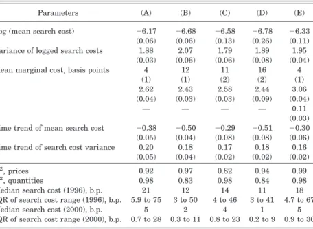
IV.B. Identification

The market share equations (7) show how we can map from observed market shares to the c.d.f. of the search cost distribution evaluated at the critical values. If we know (or assume) the sampling probabilities ␳j, then using observed market shares to

solve the linear system (7) forG(c₁), . . . ,G(cN⫺1) and using the

fact that G(cN) ⫽ 0 gives all critical values of the c.d.f. If the

sampling probabilities are unknown, and must be estimated, the probabilities as well as the search cost distribution can be param-eterized as ␳(␻1) andG(c; ␻2), respectively. Given␻1 and ␻2 of

small enough dimension, observed market shares can be used to estimate these parameters.

While market share data can be mapped into the c.d.f. of the search cost distribution, the distribution itself cannot in general be traced out using only share information. This is because mar-ket shares do not generically identify the level of the critical search cost valuesc₁, . . . ,cN, only their relative positions in the

distribution. However, sharesdoidentify search cost levels in the special but often-analyzed case of homogeneous (in all attributes but price) products with unit demands, i.e., whenuj ⫽ u⬘ ⫺ pj,

whereu⬘is the common indirect utility delivered by the funds. In this case, (4) implies that

(11) cj⫽

冘

k⫽j N

␳k共u⬘⫺pk⫺共u⬘⫺pj兲兲⫽

冘

k⫽j N

␳k共pj⫺pk兲.

Now, given sampling probabilities (either known or parametri-cally estimated), c₁, . . . , cN⫺1 can be calculated directly from

observed fund prices using (11).

In the more general case where products differ in attributes other than price alone, additional information is required to iden-tify cutoff search cost values. We find this information in fund companies’ optimal pricing decisions. The logic of our approach is

(23)

straightforward. We need to recover the p.d.f. of the search cost distribution (evaluated at the cutoff points). These values enter the derivatives of the market share equations with respect to price, (10). If we assume Bertrand-Nash competition, the first-order conditions for prices (9) imply that

(12) ⳵qj共p兲

⳵pj ⫽

⫺ qj共p兲

pj⫺mcj

.

We observe prices and market shares in the data. Therefore, given knowledge of marginal costs mc_j, we can compute⳵q_j/⳵p_j

using (12). From (10), these derivatives form a system of N ⫺ 1 linear equations that can be used to recover the values of the search cost density function g(c) at the critical values c₁, . . . ,

c_N_⫺₁. If marginal costs are not known, they can be parameterized along with the search cost distribution and estimated from the price and market share data.

Once the values of the search cost c.d.f. and p.d.f. (evaluated at the cutoff search costs) have been identified, we can recover the level of these cutoff search costsc_jin the general case of hetero-geneous products. To do so, we note that by definition the differ-ence between the c.d.f. evaluated at two points is the integral of the p.d.f. over that span of search costs. This difference can be approximated using the trapezoid method; i.e.,

(13) G共cj⫺1兲⫺G共cj兲⫽0.5关g共cj⫺1兲⫹g共cj兲兴共cj⫺1⫺cj兲.

We invert this equation to express the differences between criti-cal search cost values in terms of the c.d.f. and p.d.f. evaluated at those points:

(14) cj⫺1⫺cj⫽

2关G共cj⫺1兲⫺G共cj兲兴 g共cj⫺1兲⫹g共cj兲

.

Given the critical values ofG(c) andg(c) obtained from the data above, we can recover thecj, and from these trace out the search

cost distribution.22_{In nonparametric specifications, a}

normaliza-tion is required: the demand elasticity equanormaliza-tions do not identify

22. Of course, since we only identify the search cost distribution at the cutoff valuescj, we do not identify the c.d.f. through its entire domain. Any monotoni-cally increasing function between the identified cutoff points could be consistent with the true distribution; our trapezoid approximation essentially assumes that this is linear. The approximated c.d.f. converges to the true function as the number of funds increases.

(24)

g(cN), so a value must be chosen for the density at zero-search

costs (recall that cN ⫽ 0).23

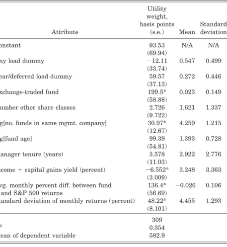
Furthermore, we can also use the critical values of the search cost distribution cj to estimate the attribute loadings ␤ in the

utility function (1). Funds’ implied indirect utilitiesujare

calcu-lated from the cj obtained above using the linear system (4).24

Since we impose a price coefficient in the utility function of⫺1, we can then estimate␤with the following regression:

(15) uj⫹pj⫽Xj␤⫹␤ageln共agej兲⫹␩j,

whereXjare observed fund attributes other than age, and␩jis a

fund-specific error term. Because the unobservable fund attribute

␰j, which is included in␩j, is likely to be correlated with fund age

(survival/longevity should be positively related to unobservable quality because high-␰jfunds are less likely to exit), we treat fund

logged age as endogenous and estimate (15) using instrumental variables. We use the instruments used by Berry, Levinsohn, and Pakes [1995] to estimate utility functions with unobservable quality. These are current-year own-fund attributes (to instru-ment for themselves) and current-year summary measures (fund counts and average levels of each nonage observable attribute) of two other sets of sector funds: other funds managed by the same company (excluding the own-fund observation), if applicable; and those managed by other companies. These two sets are unique to each fund, so instruments vary by fund-year observation. These instruments are meant to capture the effect that a fund’s relative position in attribute space (which is assumed exogenous) has on the exit decision, independent of the fund’s unobservable quality. It is interesting to note the links between our demand system and that implied by a standard discrete choice demand model like the multinomial logit (e.g., McFadden [1974]). Ours has purely vertically differentiated products, but still implies a nondegener-ate market share distribution because search cost variation across investors creates a type of horizontal differentiation. The

23. The intuition for this is that demand elasticities are determined by the actions of searchers on the margin between two funds. Given that search is responsible for spreading output shares across funds, and that changes in indirect utilities move shares on the margin only between adjacent funds, there are only

N⫺ 1 margins forNfunds. Thus, the markup/elasticity equation system only identifies the firstN⫺1 cutoff values of the search cost density function.

24. Note that in our current setup (4) implies thatu₁⫽0, so fund utility levels are expressed relative to the least desirable fund. This normalization results from our assumption that all investors purchase a fund. If we added an outside good that could be purchased without search, we could alternatively normalize this good’s utility to zero.

(25)

standard logit model also introduces products that are (almost) purely vertically differentiated, but builds in horizontal differen-tiation (and its resulting market share dispersion) directly into the preference function with the i.i.d. random utility term.

One may notice that we do not explicitly build horizontal

taste differentiation into the model. However, in subsection V.E we consider an extension that allows the investor population to be horizontally differentiated according to their mutual fund pur-chase channel. Further, we could in principle also build horizon-tal differentiation into our model by allowing investors’ tastes for fund attributes to be drawn from a parametrizable distribution, as in Berry, Levinsohn, and Pakes [1995]. Identification of the taste distributions’ parameters would require across-market vari-ation in the choice sets faced by investors. However, to empiri-cally separate taste heterogeneity from search cost differences in our model, we would also need to observe something that moves the investor search cost distributionindependentlyof tastes. Un-fortunately, our data do not offer a source of such variation, and as such we cannot directly test for the presence of general forms of horizontal taste variation.

V. ESTIMATION

V.A. The Basic Model

Our approach to estimating the model is to build up from the simplest version of the model, adding complexities (sometimes at the cost of parametric assumptions) as we go along, and compare the performance of the various versions in explaining the data.

We begin by assuming that funds are homogeneous: the only characteristic that matters to S&P 500 index fund investors is price. As noted above, homogeneity implies that u_j ⫽ u⬘ ⫺ p_j, where u⬘ is common to all funds, and given sampling probabili-ties, the cutoff search cost values can be computed directly from observed prices.

Consider the case where funds have equal sampling proba-bilities; i.e.,␳j⫽ 1/N@j. In this case the market share equations

(7) simplify to

(16) qj⫽

1

N⫹

冘

k⫽1 j⫺1

1

共N_⫺k_⫹1兲共N_⫺k兲G共ck兲⫺

1

共N_⫺j_⫹1兲G共cj兲.

As noted above, this system nonparametrically identifies the c.d.f.

(26)

of the search cost distribution. The implied G(cj) values, when

combined with the computedcjfrom the version of (4) with␳j⫽

1/N @janduj⫽ u⬘ ⫺ pj, would allow us to trace out the search

cost distribution.

However, this simple version of the model is rejected straightaway by the data. To see why, note that when sampling probabilities are equal and funds homogeneous, there will be a negative and monotonic relationship between price and market share. A glance at Figure III, which plots the fund price versus market share (both in logs) for our funds in 2000, shows that this is not the case in the sector.25 _{While there is a clear negative}

correlation between price and market share, the relationship is far from monotonic. (Recall as an example of this departure from monotonicity that the highest-fee fund was the tenth-largest of the 85 funds in 2000.)

The rejection of this simplest version of the model indicates that fund differentiation must matter on some level. We consider two possibilities. One is that funds are perceived by investors as homogeneous, but the likelihood of “finding” a fund is a function of the fund’s attributes. This breaks the basic model’s implication of monotonicity between fund price and market share by letting certain higher-priced funds be sampled with a higher relative probability than some of their lower-priced competitors. The sec-ond possibility, already alluded to above, is that investors view funds as differentiated in nonprice characteristics. A higher-priced fund may then have a larger market share than its cheaper competitor because it provides other attributes investors value. We consider both of these more complex versions in turn.

V.B. Unequal Sampling Probabilities

To allow sampling probabilities ␳j to vary across funds, we

use the following functional form specification:

(17) ␳j⫽

Zj

␣

⌺kN⫽1Zk

␣,

where Zjis an index of fund level observables that influence the

probability than the fund sampled. The parameter␣captures any nonlinearities. What should enter intoZj? If sampling

probabil-ities do differ, they are likely correlated with a fund’s market-place exposure. Since the modeled search process stylizes a very

25. Other years show a similar pattern; we choose 2000 because it had the largest number of funds.

(27)

FIGUREIII

Log Price Versus Log Market Share, 2000

The figure plots for retail S&P 500 index funds in 2000 the natural logarithm of market share versus the natural logarithm of fund price. Market shares are based on total fund assets, and price are calculated as annual fees plus one-seventh of total loads (expressed in basis points). See Data Appendix for details.

429

STUDY

OF

S&P

500

INDEX

FUNDS