Population Aging and its effect on a Japanese Economy
Taiwan-Japan Joint Seminar
2011.12.16
Hiroshi Yoshida Tohoku University
1. Objective
The objective of this study is to confirm the effect of aging on the Japanese economy. In this study, we will focus on the following three points:
(1) The effect of the aging on capital accumulation (2) The effect of the aging on labor supply
(3) The effect of the aging on trade balance
2. Effect on capital accumulation
2.1 Basic theory
Based on the life-cycle model, saving is incurred by younger generation while dissaving is incurred by elder generation. This means that aging will affect Japanese net saving negatively. Then, capital accumulation may decrease.
We assume that national capital will accumulate with,
K(t)=(1-δ)K(t-1)+I(t). (1)
In the financial market, the supply of capital via saving should balance with the demand for capital via investment.
I(t)=S(t). (2)
Following the life-cycle hypothesis, the saving is a function of the population structure,
S(t)=F(N(t, yng), N(t, old)), (3) where,
N(t,yng): Number of working-age population (age 15-64). N(t,old): Number of elder population age over 65.
With the saving function and the equation K(t), we specify the capital accumulation function as,
K(t+1)= β1 N(t, yng) + β2 N(t,old) + γ K(t). (4)
Equation 1
============
Method of estimation = Ordinary Least Squares Dependent variable: K
Current sample: 2 to 29 Number of observations: 28
Mean of dep. var. = .274E+07 Durbin-Watson = .689 [<.001] Std. dev. of dep. var. = .528E+06 Durbin's h = 3.55 [.000] Sum of squared residuals = .506E+12 Durbin's h alt. = 4.76 [.000] Variance of residuals = .202E+11 Jarque-Bera test = 4.77 [.092] Std. error of regression = .142E+06 Ramsey's RESET2 = 41.8 [.000] R-squared = .933 F (zero slopes) = 174. [.000] Adjusted R-squared = .927 Schwarz B.I.C. = 375.
LM het. test = .069 [.793] Log likelihood = -370. Estimated Standard
Variable Coefficient Error t-statistic P-value K(-1) .896 .056 15.9 ** [.000] NY 5.95 1.78 3.35 ** [.003] NO -9.46 5.31 -1.78 * [.087]
The result suggests that the working-age population (age 15-64) causes an increase in capital accumulation, the elder (over age 65) generation will, however, cause a decrease in national capital. In other words, the Japanese national capital will decrease because of future aging.
0 5 10 15 20 25 30 1.5e6
1.75e6 2e6 2.25e6 2.5e6 2.75e6 3e6 3.25e6 3.5e6
@FIT K
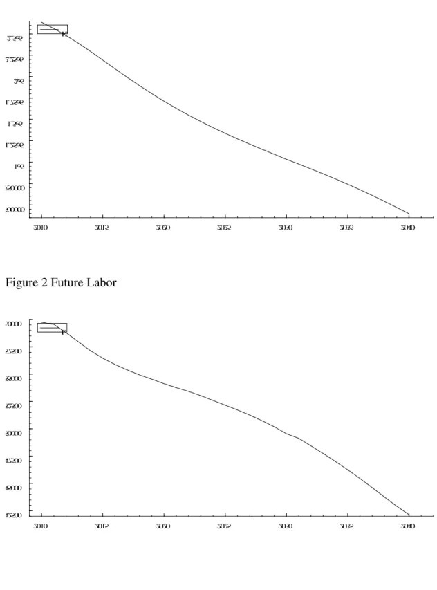
3. Effect on labor force
It is said that the aging will reduce the working-age population. This means that the future labor supply will decline if the labor participation rate will not change dramatically. Using the historical data of the population age 15-64 and the number of employed person, we obtained the labor supply function,
The result says that in Japan about 73.5 % of working-age population is employed. Based on the equation, we estimate the future labor supply with the population projection by the Japanese government.
Equation 2
============ Method of estimation = Ordinary Least Squares Dependent variable: L
Current sample: 1 to 29 Number of observations: 29
Mean of dep. var. = .622E+05 LM het. test = 17.7 [.000] Std. dev. of dep. var. = .295E+04 Durbin-Watson = .063 [<1.00] Sum of squared residuals = .999E+08 Jarque-Bera test = 1.38 [.501] Variance of residuals = .357E+07 Ramsey's RESET2 = 3.11 [.089] Std. error of regression = .189E+04 Schwarz B.I.C. = 261.
R-squared = .633 Log likelihood = -259. Adjusted R-squared = .633
Estimated Standard
Variable Coefficient Error t-statistic P-value NY .735 .414E-02 178. ** [.000]
0 5 10 15 20 25 30
56000 57000 58000 59000 60000 61000 62000 63000 64000 65000 66000
we estimate a macro production function of GDP.
0 5 10 15 20 25 30
1.6 1.7 1.8 1.9 2.0 2.1
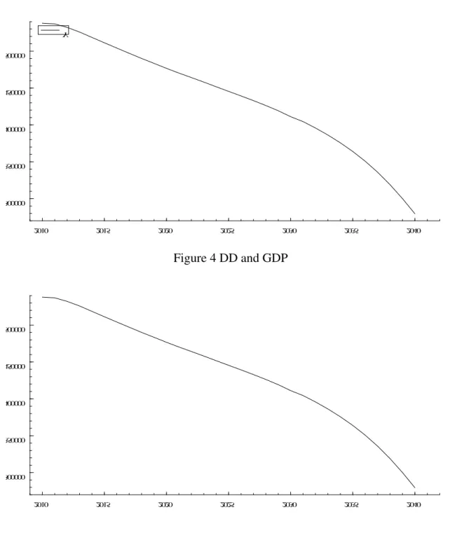
5. Effect on trade balance
We assume the equilibrium of aggregate supply and aggregate demand as follows:
AS = AD
GDP+IM = DD+EX
GDP = DD+EX-IM
GDP = DD+NX
NX = GDP-DD (8)
DD: Domestic Demand
By estimating future domestic demand (DD), we can obtain the future net export using the estimated future GDP. Now, Japan has the positive net export, the future decline of the GDP will change the net export to be negative.
Using the historical record from the SNA of Japan, we calculate DD by subtracting NX form GDP. Then, we regress DD using persons in younger and older generations.
Equation 4
============
Method of estimation = Ordinary Least Squares Dependent variable: DD
Current sample: 1 to 29 Number of observations: 29
Mean of dep. var. = .435E+06 LM het. test = 6.10 [.014] Std. dev. of dep. var. = .835E+05 Durbin-Watson = .097 [<.000] Sum of squared residuals = .542E+11 Jarque-Bera test = 1.90 [.387] Variance of residuals = .201E+10 Ramsey's RESET2 = 172. [.000] Std. error of regression = .448E+05 F (zero slopes) = 70.2 [.000] R-squared = .731 Schwarz B.I.C. = 354.
Adjusted R-squared = .721 Log likelihood = -351. Estimated Standard
Variable Coefficient Error t-statistic P-value NY 2.72 .351 7.75 ** [.000] NO 10.9 1.51 7.22 ** [.000]
6. Future simulation
Based on the equations estimated above, we will make a simulation to see the effect of the aged society on the future Japanese economy.
GDP=Y=F(K, L, t) K=K(Nyng, Nold, K-1) L= L(Nyng, Nold) DD= L(Nyng, Nold, Y) NX=GDP-DD
The results are shown in table 1 and figure 1.
7. Summary
1) Aging will lead to dissaving among the elder generation. This affects Japan’s capital accumulation negatively.
2) The simultaneous reduction of the capital and labor supply reduces the GDP of Japan continuously.
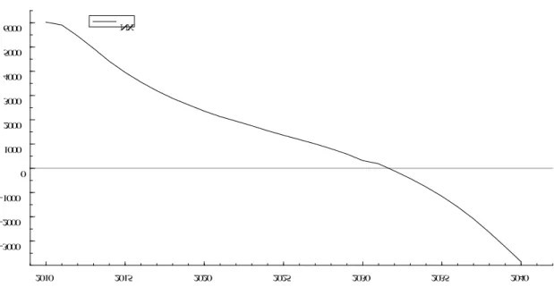
3) The simulation suggests that Japan will be faced with trade deficit after the year 2032. This means that Japan’s capital exporting will stop on the near future.
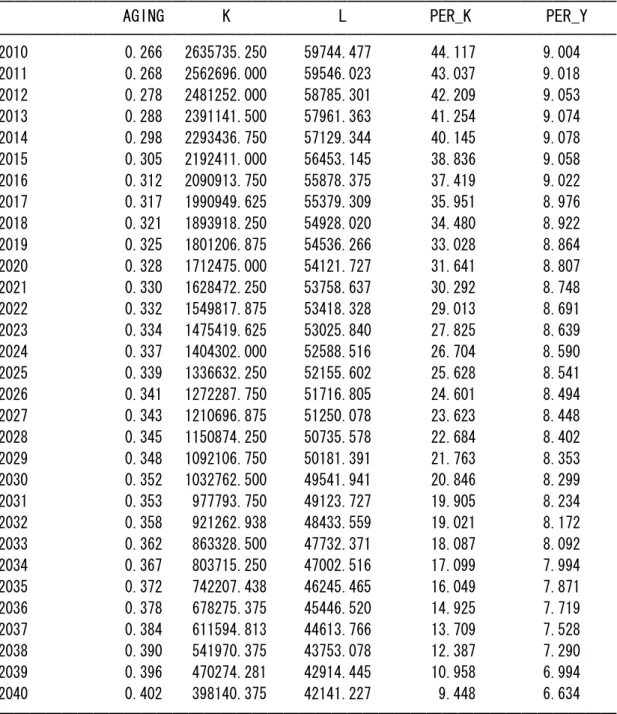
Table 1 Result of future value
――――――――――――――――――――――――――――――――――――――― AGING K L PER_K PER_Y
――――――――――――――――――――――――――――――――――――――― 2010 0.266 2635735.250 59744.477 44.117 9.004 2011 0.268 2562696.000 59546.023 43.037 9.018 2012 0.278 2481252.000 58785.301 42.209 9.053 2013 0.288 2391141.500 57961.363 41.254 9.074 2014 0.298 2293436.750 57129.344 40.145 9.078 2015 0.305 2192411.000 56453.145 38.836 9.058 2016 0.312 2090913.750 55878.375 37.419 9.022 2017 0.317 1990949.625 55379.309 35.951 8.976 2018 0.321 1893918.250 54928.020 34.480 8.922 2019 0.325 1801206.875 54536.266 33.028 8.864 2020 0.328 1712475.000 54121.727 31.641 8.807 2021 0.330 1628472.250 53758.637 30.292 8.748 2022 0.332 1549817.875 53418.328 29.013 8.691 2023 0.334 1475419.625 53025.840 27.825 8.639 2024 0.337 1404302.000 52588.516 26.704 8.590 2025 0.339 1336632.250 52155.602 25.628 8.541 2026 0.341 1272287.750 51716.805 24.601 8.494 2027 0.343 1210696.875 51250.078 23.623 8.448 2028 0.345 1150874.250 50735.578 22.684 8.402 2029 0.348 1092106.750 50181.391 21.763 8.353 2030 0.352 1032762.500 49541.941 20.846 8.299 2031 0.353 977793.750 49123.727 19.905 8.234 2032 0.358 921262.938 48433.559 19.021 8.172 2033 0.362 863328.500 47732.371 18.087 8.092 2034 0.367 803715.250 47002.516 17.099 7.994 2035 0.372 742207.438 46245.465 16.049 7.871 2036 0.378 678275.375 45446.520 14.925 7.719 2037 0.384 611594.813 44613.766 13.709 7.528 2038 0.390 541970.375 43753.078 12.387 7.290 2039 0.396 470274.281 42914.445 10.958 6.994 2040 0.402 398140.375 42141.227 9.448 6.634
―――――――――――――――――――――――――――――――――――――――
――――――――――――――――――――――――――――――――――――――― TPER_Y Y DD NX
――――――――――――――――――――――――――――――――――――――― 2010 4.860 537953.438 531930.188 6023.250
2011 4.850 536976.000 531069.375 5906.625 2012 4.806 532163.375 526708.750 5454.625 2013 4.751 525935.438 520991.563 4943.875 2014 4.686 518601.656 514190.844 4410.813 2015 4.624 511352.719 507400.094 3952.625 2016 4.564 504156.844 500606.125 3550.719 2017 4.506 497066.563 493871.156 3195.406 2018 4.451 490082.875 487201.844 2881.031 2019 4.401 483426.594 480811.781 2614.813 2020 4.352 476665.938 474310.875 2355.063 2021 4.306 470282.250 468152.406 2129.844 2022 4.267 464244.719 462300.750 1943.969 2023 4.228 458084.250 456333.531 1750.719 2024 4.188 451734.594 450188.000 1546.594 2025 4.151 445479.813 444119.594 1360.219 2026 4.116 439276.438 438092.094 1184.344 2027 4.080 432955.719 431950.625 1005.094 2028 4.042 426283.531 425477.594 805.938 2029 4.000 419183.563 418595.281 588.281 2030 3.951 411151.156 410833.094 318.063 2031 3.914 404465.531 404280.000 185.531 2032 3.858 395779.719 395888.188 -108.469 2033 3.795 386268.750 386690.875 -422.125 2034 3.720 375720.188 376490.250 -770.063 2035 3.634 363997.063 365152.438 -1155.375 2036 3.532 350788.188 352381.781 -1593.594 2037 3.411 335871.063 337958.969 -2087.906 2038 3.268 318964.906 321609.250 -2644.344 2039 3.103 300142.719 303382.594 -3239.875 2040 2.916 279575.000 283428.500 -3853.500
――――――――――――――――――――――――――――――――――――――― unit triton yen except y. y: thousand yen.
Figure1 Future Capital
2010 2015 2020 2025 2030 2035 2040
500000 750000 1e6 1.25e6 1.5e6 1.75e6 2e6 2.25e6
2.5e6 K
Figure 2 Future Labor
2010 2015 2020 2025 2030 2035 2040
42500 45000 47500 50000 52500 55000 57500 60000
L
Figure 3 Future GDP
2010 2015 2020 2025 2030 2035 2040
300000 350000 400000 450000 500000
Y
Figure 4 DD and GDP
300000 350000 400000 450000 500000
Figure 5 Net Export
2010 2015 2020 2025 2030 2035 2040
-3000 -2000 -1000 0 1000 2000 3000 4000 5000
6000 NX
Appendix Data used
t K 15-64 65- Y L NX DD
1981 1,484,720.70 79,272 11,009 261,068.20 55,810 -2219.1 263287.3 1982 1,575,452.30 80,089 11,350 274,086.60 56,380 1919.3 272167.3 1983 1,629,378.00 80,904 11,672 285,058.30 57,330 1849.3 283209 1984 1,699,381.10 81,776 11,956 302,974.90 57,660 4867.2 298107.7 1985 1,811,019.50 82,535 12,472 325,401.90 58,070 8036.1 317365.8 1986 2,113,913.10 83,368 12,870 340,559.50 58,530 11039.4 329520.1 1987 2,579,662.10 84,189 13,322 354,170.20 59,110 13280.9 340889.3 1988 2,836,726.90 85,013 13,785 380,742.90 60,110 10561.1 370181.8 1989 3,231,062.40 85,745 14,309 410,122.20 61,280 8239.2 401883 1990 3,531,467.20 86,140 14,928 442,781.00 62,490 6237.1 436543.9 1991 3,422,746.40 86,557 15,582 469,421.80 63,690 4173.2 465248.6 1992 3,265,515.10 86,845 16,242 480,782.80 64,360 7547 473235.8 1993 3,192,859.50 87,023 16,900 483,711.80 64,500 10397.6 473314.2 1994 3,150,014.40 87,034 17,585 488,450.30 64,530 10765.5 477684.8 1995 3,079,762.50 87,260 18,277 495,165.50 64,570 9883 485282.5 1996 3,101,125.10 87,161 19,017 505,011.80 64,860 6957.7 498054.1 1997 3,118,792.30 87,042 19,758 515,644.10 65,570 2538.8 513105.3 1998 3,044,332.70 86,920 20,508 504,905.40 65,140 5757.5 499147.9 1999 2,911,152.60 86,758 21,186 497,628.60 64,620 9444 488184.6 2000 2,883,379.20 86,380 22,041 502,989.90 64,460 7892.4 495097.5 2001 2,825,349.70 86,139 22,869 497,719.70 64,120 7315.5 490404.2 2002 2,720,024.90 85,706 23,628 491,312.20 63,300 3174.2 488138 2003 2,640,378.00 85,404 24,311 490,294.00 63,160 6411.9 483882.1 2004 2,629,883.80 85,077 24,876 498,328.40 63,290 7975.5 490352.9
TSP Program options signif=3; freq a;
smpl 1981,2009;
LOAD t K Ny No Y L NX DD;
1981 1484720.70 79272 11009 261068.20 55810 -2219.1 263287.3 1982 1575452.30 80089 11350 274086.60 56380 1919.3 272167.3 1983 1629378.00 80904 11672 285058.30 57330 1849.3 283209 1984 1699381.10 81776 11956 302974.90 57660 4867.2 298107.7 1985 1811019.50 82535 12472 325401.90 58070 8036.1 317365.8 1986 2113913.10 83368 12870 340559.50 58530 11039.4 329520.1 1987 2579662.10 84189 13322 354170.20 59110 13280.9 340889.3 1988 2836726.90 85013 13785 380742.90 60110 10561.1 370181.8 1989 3231062.40 85745 14309 410122.20 61280 8239.2 401883 1990 3531467.20 86140 14928 442781.00 62490 6237.1 436543.9 1991 3422746.40 86557 15582 469421.80 63690 4173.2 465248.6 1992 3265515.10 86845 16242 480782.80 64360 7547 473235.8 1993 3192859.50 87023 16900 483711.80 64500 10397.6 473314.2 1994 3150014.40 87034 17585 488450.30 64530 10765.5 477684.8 1995 3079762.50 87260 18277 495165.50 64570 9883 485282.5 1996 3101125.10 87161 19017 505011.80 64860 6957.7 498054.1 1997 3118792.30 87042 19758 515644.10 65570 2538.8 513105.3 1998 3044332.70 86920 20508 504905.40 65140 5757.5 499147.9 1999 2911152.60 86758 21186 497628.60 64620 9444 488184.6 2000 2883379.20 86380 22041 502989.90 64460 7892.4 495097.5 2001 2825349.70 86139 22869 497719.70 64120 7315.5 490404.2 2002 2720024.90 85706 23628 491312.20 63300 3174.2 488138 2003 2640378.00 85404 24311 490294.00 63160 6411.9 483882.1 2004 2629883.80 85077 24876 498328.40 63290 7975.5 490352.9 2005 2626223.50 84422 25761 501734.40 63560 9626 492108.4 2006 2719713.50 83731 26604 507364.80 63820 6956 500408.8 2007 2811062.60 83015 27464 515520.40 64120 6348.5 509171.9 2008 2808044.50 82300 28216 504377.60 63850 8632.4 495745.2 2009 2712378.10 81493 29005 470936.70 62820 735.6 470201.1
;
regopt (STAR1=0.10 STAR2=0.05)T; Aging=no/(ny+no);
olsq K K(-1) Ny No; print @coef;
plot @fit k;
olsq L Ny; print @coef; plot @fit l; per_y=Y/L;
per_k=K/l;
lnper_y=Log(per_y); lnper_k=Log(per_k);
olsq lnper_y lnper_k c t; plot @fit lnper_y;
print @coef;
olsq dd ny no y; plot @fit dd; print @coef;
smpl 2010,2040; t=t(-1)+1;
load ny no; 81285 29412 81015 29704 79980 30745 78859 31852 77727 32934 76807 33781 76025 34450 75346 34977 74732 35380 74199 35655 73635 35899 73141 36064 72678 36131 72144 36210 71549 36307 70960 36354 70363 36371 69728 36388 69028 36438 68274 36510 67404 36670
L=0.735*Ny; plot L; per_k=K/L;
lnper_k=Log(K/L);
lnper_y=0.4396*lnper_k-24.391+0.0124*t; plot lnper_y;
per_y=exp(lnper_y); plot per_y;
Y=per_y*L; plot y;
Tper_y=y/(no+ny); plot tper_y;
Aging=no/(ny+no);
dd= -0.00541*Ny+0.304*No+0.973*y; plot dd;
NX=Y-dd; plot nx; plot y dd;
print aging k l per_k per_y tper_y y dd nx;