mdp07001 Recent site activity Junji Kageyama's Homepage

Incentive Problem in Intergovernmental Transfers: Differences

between Two Infinitely Iterated Leadership Models

^∗

TAKAHASHI Hiromasa ^†, TAKEMOTO Toru^‡, SUZUKI Akihiro^§

The Economic Society of Meikai University Discussion Paper, DP2007-001

Abstract

The authors deal with a certain type of timing problem in the allocation of cen- tral government subsidies to local governments, called the “soft budget constraint problem” in fiscal science. Many studies have claimed that central government incentives provided to bail out local governments cause distortion. This paper will show that this assertion is problematic by assuming that the central and local governments have an infinite-horizon view and by adopting the Markov perfect equilibrium (MPE) as a solution concept. The two models in this paper can be interpreted as dynamic social dilemmas. One is analogous to the tragedy of the commons, e.g., Levhari and Mirman (1980). The other shares some of the features of a dynamic social dilemma, and the two models are the same barring the timing of players’ moves; despite this, the MPE behavior is quite different. By comparing these models, this paper will show that competitive restriction may improve social welfare.

∗ This work was supported by Grant-in-Aid for Scientific Research (C) (18530226). We thank Nobuo Akai, Jun-ichi Itaya, Kazuo Mino, Hiroyuki Ozaki, and Motohiro Sato for helpful discussions and comments.

† Faculty of International Studies, Hiroshima City University, E-mail: htaka@intl.hiroshima- cu.ac.jp

‡Faculty of Economics, Meikai University, E-mail: takemoto@meikai.ac.jp

§ Faculty of Literature and Social Sciences, Yamagata University, E-mail: asuzuki@human. kj.yamagata-u.ac.jp

1 Introduction

In the paper, we deal with a certain type of timing problem in the allocation of subsidies by the central government to local governments. We will show that the path of occurrence of the distortion caused by subsidization varies according to the timing of the subsidy offer. Our timing problem is called “time inconsistency” in macroeconomics, which is addressed by Kydland and Prescott (1977). They conclude that policymakers fail to commit to a low inflation rate in advance since the level of unemployment is reduced by effecting high inflation. The same problem is called a “soft budget constraint (SBC) problem” in fiscal science. A considerable section of the literature on the SBC problem supports that central-government- sponsored bailouts for local governments through subsidies cause distortion. This paper will attempt a different interpretation of the SBC problem by assuming that central and local governments have an infinite-horizon view, which is standard in macroeconomics. Moreover, we will find that our models have the same structure as social dilemmas.

In fiscal science, it has been indicated that the interregional redistribution policy of the central government causes incentive problems such as excess expen- diture or excess debt. These problems are referred to as SBCs, the origin of which is related to the analyses of distortions that resulted from bailouts of loss-making state-owned enterprises in a socialized economy (see Kornai (1979, 1980)).

SBC has been applied to the problem of subsidies provided to local governments by the central government and has been discussed as a cause of distortions resulting from the redistribution. For example, Wildasin (1997) and Akai and Sato (2005) attempt an analysis of a situation wherein the central government provides ex-post subsidy relief to areas in which consumption of public and private goods is in short supply compared with other areas. They conclude that under such conditions, the budget constraints of local governments “soften,” and the supply of public goods and the rate of tax are distorted.

However, this result is not necessarily found only in a single-year model. Good- speed (2002) can be considered to suggest this fact. If relations between the central and local governments are maintained over the years, present decision-making by

local governments should have an influence on future decisions on central gov- ernment subsidies. It can be also said that the present decision on the subsidy by the central government should have an influence on future decision-making of local governments. The point is that even if there is no distortion resulting from subsidy problems in the single period model, distortion can be caused by simply shifting those problems to a multiperiod model. Furthermore, compared to one-period model generating distortion, there could be different mechanisms generating distortion in some multiperiod models.

Taking this into account, we analyze problems of subsidy systems from central to local governments in “infinitely iterated leadership models.” We use the term

“infinitely iterated model” in the sense that this model is not simply a repeated game but has a state variable (vector in our model). Some of the literature refers to such models as “difference games,” e.g., de Zeeuw and van der Ploeg (1991). While differential games are dynamic games in continuous time, difference games are dynamic games in discrete time. We use difference games to describe the timing of all the players’ behaviors with fair accuracy. In this paper we suppose that there are two situations wherein local governments’ decision-making on the supply of local public goods and on local bond issues, and the central government’s decisions on the delivery of subsidies are made with different timings. In one situation, the central government decides the subsidy as the first move of every period, and the local governments then supply local public goods; this is called the “central leadership (CL)” model. In the other situation the order is inverted; this is called the “decentralized leadership (DL)” model.

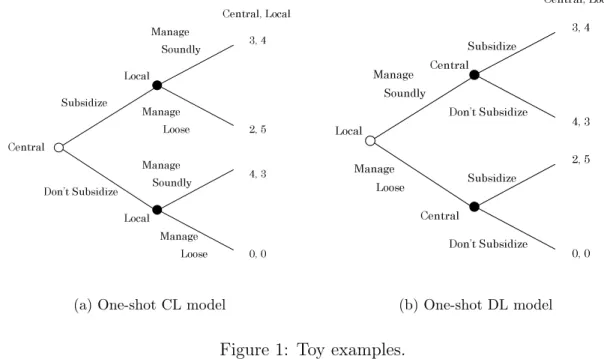
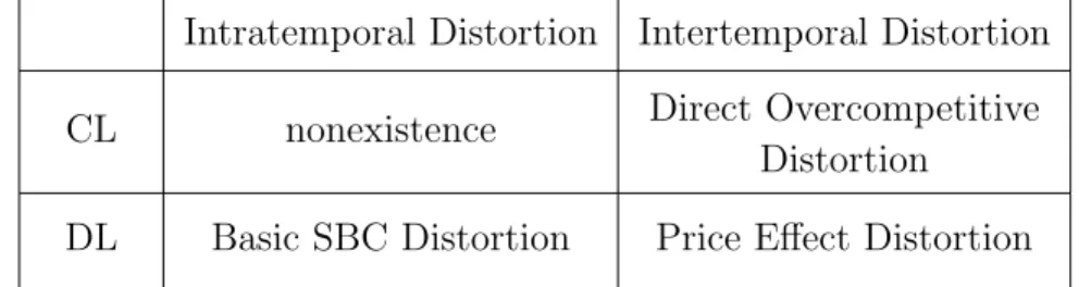
The CL and DL models are used to explain the SBC problem between central and local governments. Toy examples of these are described in Figure 1. In the subgame perfect equilibrium of the CL model, the central government plays “don’t subsidize” and the local government plays “manage soundly.” By contrast, the local government plays “manage loose” and the central government plays “subsi- dize” in the equilibrium of the DL model. Therefore, the above examples show that a distortion occurs if the central government can, before choosing an action, observe the actions of the local government. This is the usual explanation of the

Central

Local

Local Subsidize

Don’t Subsidize

Manage Soundly

Manage Soundly Manage

Loose

Manage

Loose 0, 0 Central, Local

4, 3 2, 5 3, 4

(a) One-shot CL model

Central Local

Subsidize

Don’t Subsidize Manage

Soundly

Manage Loose

0, 0 Central, Local

4, 3 2, 5 3, 4 Central

Don’t Subsidize

Subsidize

(b) One-shot DL model

Figure 1: Toy examples.

SBC problem in the context of intergovernmental transfer, hereinafter called “ba- sic SBC distortion.” On the other hand, in the above CL model no inefficiency is found.

However, inefficiency may occur in multiperiod CL models. In our model, each local government decides its local tax and local bonds, and the central government decides the subsidies to the local governments. In the model, an intertemporal distortion may occur, that is, the local government issues excess bonds to achieve a larger current consumption. In actuality, in two-period versions, we can show that an intertemporal distortion will occur even in the CL model since, in the first period, the local governments anticipate the second period’s subsidies from the central government, which depend on the outstanding local bonds in the first period.¹ On the other hand, an intertemporal distortion and the basic SBC dis- tortion will occur in the DL model. Moreover, we can show that the sum of the two types of distortion in a DL model is more aggravated than the intertemporal distortion in a CL model.

However, it is problematic that we admit to the above outcome in two-period

1We will show that an intertemporal distortion occurs in the infinitely iterated CL model. However, the reason for the distortion is quite different from that in the two-period CL model.

models because of the following reason: In general, an agent with a concave utility function equalizes its consumption for all periods in a multiperiod model. Thus, an increase or decrease in consumption in a single period due to intertemporal distortion may affect the consumption in all the other periods. If this effect, which occurs in all periods, accumulates and the intertemporal distortion in a CL model is more than that in a DL model, the welfare in the CL model may fall below that in the DL model.

For this reason, we should consider longer-period models. Consequently, we will deal mainly with infinite-period models in this paper; the reasons are as follows. First, infinite-period models have been used to analyze agent behavior in macroeconomics since Ramsey (1928). In particular, it seems plausible that a governments actions would be based on a long-term perspective. The second reason is to avoid the same effect as in any finitely repeated prisoner’s dilemma, which is caused by the existence of a final period.

The Markov perfect equilibrium (MPE) is adopted as a solution concept in this paper. This concept is a refinement of the Nash equilibrium and has a high suit- ability to dynamic programming. Furthermore, Maskin and Tirole (2001) states that the MPE has many favorable properties, e.g., it requires only the coarsest of information. Any individually rational outcome is achieved by a trigger strategy as a subgame perfect equilibrium in an infinitely repeated game. On the other hand, no deviant player may be penalized in our setting as the Markov strategy only depends on the state variable in the adjacent period. Hence, it is impossible to detect any deviation if a state variable of any value is possible in period zero. Therefore, it is also impossible to penalize the deviant player without adopting a strategy that immediately penalizes in case the state variable attains a particular value even in period zero. We rationalize the use the MPE as follows: Although the folk theorem may predict Pareto-efficient outcomes, some of the literature on pub- lic finance suggest the inefficiency of local governments, e.g., Pettersson-Lidbom and Dahlberg (2005) and Doi and Ihori (2006). Doubtless, it is unknown which outcome is realized since the folk theorem also predicts a considerable number of other inefficient outcomes. Moreover, although every deviant player must be

penalized by all the other players in any trigger strategy (or an analogous strategy such as a stick-and-carrot strategy) equilibrium, in a practical sense, no (probably local) government seems to be penalized by the other governments when it raises its local taxes and/or increases its public debt.

The models in this paper can be interpreted as dynamic social dilemmas. Lev- hari and Mirman (1980) and Dutta and Sundaram (1993) study dynamic common- property resource games. Velasco (2000) studies a model concerning fiscal policy that is essentially identical to that in the above literature. Though the infinitely iterated CL model is different from these models, it eventually has a solution that indicates the same behavior as that of these models. On the other hand, although the infinitely iterated DL model is the same as an infinitely iterated CL model barring the timing of the players’ move and also shares some of the features of a social dilemma, its equilibrium behavior is different from that described the above literature.

Ortigueira (2006) has studied the relation between the optimal tax policy and the timing of actions. Ortigueira (2006) has the same purpose as our paper, in the sense that it attempts to study the importance of the timing of actions by comparing MPEs. Although Ortigueira (2006) has taken a numerical approach, our models will be solved analytically.

This paper is organized as follows: In Sections 2 and 3, we introduce infinitely iterated CL and DL models and calculate the MPEs. Section 4 is devoted to the description of finitely iterated models and attempts to justify the infinitely iterated models of the previous sections. In Section 5, we attempt a comparison between the infinitely iterated CL and DL models of the previous sections. Section 6 concludes this paper, and the last section includes some proofs.

2 Infinitely Iterated CL Model

The infinitely iterated CL model (or “CL model” for short) represents the following situation: In each year, the central government decides the subsidies to residents in each region before the local governments decide the outstanding local bonds and local taxes; and this process is repeated over many years.

2.1 Definition of the Game and the Equilibrium

Environment The economy contains two regions: region 1 and region 2. There are the central and two local governments. A typical region or a local government is represented by i. Each region consists of a representative resident with an infinite lifespan. The resident in region i earns one unit of income every period and his or her preference is represented by a utility function,

Uⁱ({cⁱ_t}t∈T, {g_tⁱ}t∈T) =

∞

∑

t=1

β^t−1uⁱ(cⁱ_t, g_tⁱ),

where T = {1, 2, · · · }, cⁱ_t indicates private goods consumption, and gⁱ_t indicates the local public goods² supply in period t. They are assumed to be nonnegative. In each period, the players’ decisions in the stage game are as follows:

(1) The central government decides subsidies (z_t¹, z_t²) to each resident to satisfy z_t¹+ z_t² = 0. (First move in period t.)

(2) Both local governments simultaneously decide outstanding local bonds xⁱ_t and local taxes yⁱ_t. (Second move in period t.)

(3) Private goods consumption cⁱ_t and local public goods supply g_tⁱ are realized, where cⁱ_t and g_tⁱ satisfy the following equations:

cⁱ_t = 1 − y_tⁱ+ z_tⁱ, (1)

g_tⁱ = yⁱ_t+ xⁱ_t−(1 + r)xⁱ_t−1. (2)

In the last equation, r ∈ (0, 1) is an interest rate that is invariant with time and is set for all regions. Assume that the sum of the outstanding local bonds is constrained by the discounted sum of the future incomes in both regions (²_r); namely,

(∀t ∈ T ) x¹_t−1+ x²_t−1 ≤ ²

r^{, (3)}

where x¹₀ and x²₀ are given for all the residents in the economy. In this economic environment, if x¹_τ−1+ x²_τ−1 = ²_r for some τ ∈ T , x¹_t+ x²_t = ²_r for all t ≥ τ because of the budget constraint,

2Strictly speaking, the goods are not public goods. We could give gtⁱ the properties of public goods; however, this would add unnecessary complexity to our assertion.

(∀t ∈ T ) 2 + x¹_t + x²_t − (1 + r)(x¹_t−1+ x²_t−1) = c¹_t + c²_t + g¹_t + g_t² ≥ 0. Furthermore, the sum of local taxes must be smaller than or equal to 2, namely,

(∀t ∈ T ) y_t¹+ y_t² ≤ 2, (4)

since z_t¹+ z_t² = 0 and cⁱ_t= 1 − y_tⁱ+ z_tⁱ ≥ 0 for i = 1, 2.

The central government aims to make the social welfare, ^∑2_i=1θⁱUⁱ({cⁱ_t}t∈T, {g_tⁱ}t∈T), as large as possible, where θ¹ ≥ 0, θ² ≥ 0; while local government i aims to maximize Uⁱ({cⁱ_t}t∈T, {gⁱ_t}t∈T).

History Let B ⊂ (R^T)2, Q ⊂ (R^T)2 and S ⊂ (R^2)T denote a set of the history of admissible outstanding local bonds, that of local taxes, and that of subsidies from the central to local governments, respectively.

For a history of subsidies z = ((z₁¹, z₁²), (z₂¹, z²₂), · · · ) ∈ S, let ztdenote a history of subsidies from the first to period t, that is, ((z₁¹, z₁²), (z¹₂, z₂²), · · · , (z_t¹, z_t²)). Sim- ilarly, for a history of local taxes (local bonds) y ∈ Q (x ∈ B), yt (xt−1) denotes the first t elements of the history. For all t ∈ T , sets of all these elements are denoted by St, Qt, and Bt−1. Note that Bt is a subset of (R^{t+1)2, while Q}t and St

are subsets of (R^t)2 and (R^2)t, respectively.³

We define the sets of histories (H, Ht, and H^C_t ) as follows. H ≡ B × Q × S,

Ht ≡







B0 if t = 0

Bt× Qt× St if t ∈ T ^,

H^C_t ≡







B₀× S₁ if t = 1 Bt−1× Qt−1× St if t ∈ T /{1}.

Ht denotes the set of histories up to the second move in period t, and H_t^C, the set of histories up to the first move in period t.

Strategy Set The local governments’ strategy sets A^C1 and A^C2and the central government’s strategy set A^C0 are defined as follows. For i = 1, 2,

3The formal definitions of B, Q, S, B^t−1, Q^t, and S^tmay be found in Appendix A.

A^Ci ≡ ^{((b1, q1), (b2, q2), · · · ) ∈ Πt∈T

( R^HtC)2

¯

¯

¯ (∀t ∈ T )(∀h ∈ H

C t ⁾

1 − qt(h) + z_tⁱ ≥ 0, qt(h) + bt(h) − (1 + r)xⁱ_t−1 ≥ 0 where

h = ((x¹₀, · · · , x¹_t−1), (x²₀, · · · , x²_t−1), yt−1, ((z₁¹, z₁²), · · · , (z_t¹, z_t²)))^}, A^C0 ≡ ^{((s¹₁, s²₁), (s¹₂, s²₂), · · · ) ∈ Πt∈T_(R^Ht−1)^2¯¯¯ (∀t ∈ T )(∀h ∈ ^Ht−1)

s¹_t(h) + s²_t(h) = 0^}.

For given ((s¹₁, s²₁), (s¹₂, s²₂), · · · ) ∈ A^C0, sⁱ_{t ∈ R}^Ht−1 represents a function that as- signs subsidies to the resident in region i in period t. In period t, the central government decides subsidies depending on the history up to period (t − 1). On the other hand, for given ((b1, q1), (b2, q2), · · · ) ∈ A^Ci, bt ∈ R^{Hℓt (q}t ∈ R^{Hℓt) repre-} sents the outstanding local bonds (local taxes) in period t. In period t, the local governments decide the outstanding local bonds and local taxes depending on the history up to period (t − 1) and on the central government’s decision in period t. However, for some t ∈ T , ((b¹₁, q¹₁), (b¹₂, q₂¹), · · · ) ∈ A^C1, ((b²₁, q₁²), (b²₂, q₂²), · · · ) ∈ A^C2, and h ∈ H^C_t, it may be that b¹_t(h) + b²_t(h) > ²_r. Therefore, to satisfy (3), if b¹_t(h) + b²_t(h) > ²_r, the outstanding local bonds (xⁱ_t) and local taxes (y_tⁱ) of local government i in period t are assumed to be⁴

xⁱ_t = −1 − z_tⁱ+^{1 + r} 2

( 2 r ^{+ x}

i t−1^{− x}

j t−1

)

, (5)

yⁱ_t = 1 + z_tⁱ− ^{1 + r} 4

( 2 r ^{− x}

1

τ−1^{− x2}τ−1

)

. (6)

Definition of Equilibria Let A^C denote A^C0× A^C1× A^C2. When a combina- tion of strategies, a = (a⁰, a¹, a²) ∈ A^C, and a history up to period τ , h ∈ Hτ, are given, the sequence of consumption in region i after period (τ + 1), wⁱ(a, h) = ({cⁱ_t}t∈T, {gⁱ_t}t∈T), can be determined uniquely for i = 1, 2. For example, when a⁰ = ((s¹₁, s²₁), (s₂¹, s²₂), · · · ), aⁱ = ((bⁱ₁, q₁ⁱ), (bⁱ₂, qⁱ₂), · · · ), h = (( x¹_τ, x²_τ), (y_τ¹, y²_τ), zτ), and x¹_τ = (xⁱ₀, · · · , xⁱ_τ), c_tⁱ and g_tⁱ are determined by (1) and (2), where xⁱ₀ = xⁱ_τ;

4 Under this determination of xⁱt and yⁱt, x¹t + x²t = ²_r, ytⁱ + xⁱt− (1 + r)xⁱt₋₁ ≥ 0, and 1 − yⁱt+ ztⁱ≥ 0. Moreover, cⁱT = gⁱT = 0 for T ≥ t + 1 and for i = 1, 2. The equilibrium strategy presented in Proposition 2 necessarily satisfies b¹t(h) + b²t(h) ≤ ²r. The result does not depend on the method used to determine xⁱt and ytⁱ when b¹t(h) + b²t(h) > ²r, as long as they satisfy x¹t+ x²t =²r, yⁱt+ xⁱt− (1 + r)xⁱt₋₁≥ 0, and 1 − yⁱt+ zⁱt≥ 0.

and for t ∈ T at which b¹_τ+t + b²_τ+t ≤ ²_r, xⁱ_t, y_tⁱ, and z_tⁱ are defined in the following manner:⁵

xⁱ_t = bⁱ_τ+t(h^ℓ_t), y_tⁱ = qⁱ_τ+t(h^ℓ_t), z_tⁱ = sⁱ_τ+t(ht−1), zτ+t = (zⁱ_τ+t−1, (z_t¹, z_t²)), h₀ = h, h^ℓ_t = (( x¹_τ+t−1, x_τ+t−1² ), y_τ+t−1¹ , y_τ+t−1² , z_τ+t),

xⁱ_τ+t = (xⁱ_τ+t−1, xⁱ_t), yⁱ_τ+t = (yⁱ_τ+t−1, y_tⁱ), ht = (x¹_τ+t, x²_τ+t, y¹_τ+t, y²_τ+t, zτ+t). In a similar manner, when a combination of strategies and the history up to the first move in period τ , h ∈ H_t^C, are given, the sequence of consumption after the period τ , wⁱ(a, h), can be uniquely determined.

Definition 1 A combination of strategies (a^0∗, a^1∗, a^2∗) ∈ A^Cis a subgame perfect equilibrium of the CL model if it satisfies the following conditions:

(∀t ∈ T ) (∀h ∈ Ht−1) a^0∗ ∈ arg max

a∈A^C0

∑

i=1,2

θⁱUⁱ(wⁱ((a, a^1∗, a^2∗), h)), (∀t ∈ T ) (∀h ∈ H^C_t ) a^1∗ ∈ arg max

a∈A^C1U

1_(w1_((a0∗_{, a, a}2∗_{), h)),}

(∀t ∈ T ) (∀h ∈ H^C_t ) a^2∗ ∈ arg max

a∈A^C2U

2_(w2_((a0∗_{, a}1∗_{, a), h)).}

Furthermore, the MPE is defined. When functions f ∈ R^H0 and e ∈ R^{HC1 are} given, the functions f = (f1, f2, · · · ) ∈ Πt∈TR^{Ht−1 and e = (e}1, e2, · · · ) ∈ Πt∈TR^HCt can be uniquely determined in the following manner:

f1 = f and e1 = e (7)

(∀t ∈ T ) ft+1(x¹_t, x²_t, y_t¹, y_t², zt) = f (x¹_t, x²_t), (8) (∀t ∈ T ) et+1(x¹_t, x²_t, y¹_t, y²_t, zt+1) = e(x¹_t, x²_t, z_t+1¹ , z_t+1² ), (9) where (x¹_t, x²_t) ∈ Bt, x_tⁱ = (xⁱ₀, xⁱ₁, · · · , xⁱ_t), yⁱ_t∈ Qt, and zt= ((z₁¹, z₁²), · · · , (z¹_t, z²_t))

∈ St. Using (7) and (8), one can construct a strategy a ∈ A^C0 from a combination of functions (s¹, s²_{) ∈ (R}^H0)² if s¹+ s² = 0. Hence, we state that a combination of functions (s¹, s²_{) ∈ (R}^H0)² satisfying s¹ + s² = 0 is a Markov strategy of the central government.

Similarly, for i = 1, 2, one can construct a strategy a ∈ A^Cifrom a combination of functions (b, q) ∈ (R^H1C)2 if 1−q(h)+zⁱ ≥ 0 and q(h)+b(h)−(1+r)xⁱ ≥ 0, where

5If b¹τ +t+ b²τ +t> ²_r, xⁱt and ytⁱ are determined through (5) and (6).

h = (x¹, x², z¹, z²), by using (7) and (9). Hence, we state that a combination of functions (b, q) ∈ (R^H0)2 satisfying 1 − q(h) + zⁱ ≥ 0 and q(h) + b(h) − (1 + r)xⁱ ≥ 0 is a Markov strategy of local government i.

Definition 2 A combination of Markov strategies ((s¹, s²), (b¹, q¹), (b², q²)) is an MPE of the CL model if (a⁰, a¹, a²) ∈ A^C is a subgame perfect equilibrium, where a⁰ is constructed from (s¹, s²) by using (7) and (8) and, for i = 1, 2, aⁱ is con- structed from (bⁱ, qⁱ) by using (7) and (9).

Note that the MPE is subgame perfect since Markov restriction is not imposed on the definition of strategy sets. As discussed in Blanchard and Fischer (1989, Chap.11), a subgame perfect equilibrium strategy of the central government is time consistent in the sense discussed by Kydland and Prescott (1977).

In the following, we make the following assumptions.

Assumption (i) β(1 + r) < 1; (ii) uⁱ(c, g) = ln c + ln g for i = 1, 2; and (iii) θ¹ = θ² = 1.

2.2 Planning Problem

The problem of maximizing the social welfare is solved in this subsection. This problem is described in the following manner:

max

∞

∑

t=1

β^t−1

2

∑

i=1

{ln(1 − y_tⁱ+ zⁱ_t) + ln [ y_tⁱ+ xⁱ_t− (1 + r)xⁱ_t−1]} s.t 1 − y_tⁱ+ zⁱ_t≥ 0, y_tⁱ+ xⁱ_t− (1 + r)xⁱ_t−1 ≥ 0,

x¹_t + x²_t ≤ ² r^{, z}

1

t ^{+ z}t^{2 = 0, x1}0 ^{and x2}0 ^{are given.}

Let us define the function I ∈ (R+)^B0 as I(x¹, x²) = (1 + r)⁽²_r − x¹− x²). From the theory of dynamic programming,⁶ we can solve the problem and obtain the following result.

Proposition 1 There exist xⁱ_t, yⁱ_t, z_tⁱ that solve the planning problem. The gross outstanding local bonds x¹_t+ x²_t, private consumption cⁱ_t= 1 − y_tⁱ+ z_tⁱ, and public goods supply g_tⁱ = y_tⁱ+ xⁱ_t− (1 + r)xⁱ_t−1 corresponding to all the solutions are the same. Furthermore, they satisfy the following equations:

6See Stokey, Lucas, and Prescott (1989) as a standard textbook.

I(x¹_t, x²_t) = β(1 + r)I(x¹_t−1, x²_t−1), (10) y¹_t + y²_t = 2 − ^{1 − β}

2 ^I(x

1

t^{, x2}t^{), (11)}

c¹_t = c²_t = g_t¹ = g_t² = ^{1 − β} 4 ^I(x

1 t^{, x2}t^),

U¹({c¹_t, g_t¹}t∈T) = U²({c_t², g_t²}t∈T) = V^∗(x¹₀, x²₀), V^∗(x¹₀, x²₀) = ²

1 − β ^ln ( 2

r ^{− x}

1 0^{− x2}0

) + δ^∗, δ^∗ = ²

(1 − β)² {β ln β + (1 − β) ln(1 − β) + ln(1 + r) − 2(1 − β) ln 2}. I(x¹, x²) represents the net present value of the lifetime income in both regions (or the gross lifetime income for short), namely, the sum of today’s gross income and the discounted future gross income (2+²_r) minus bond redemption((1+r)(x¹+x²)). Since β(1+r) < 1, x¹_t+x²_t → ²_r and I(x¹_t, x²_t) → 0 as t → ∞ in the optimal solution. When the gross lifetime income increases, the current consumption also in- creases. For this purpose, the net amount of bond issuance increases and, at the same time, the local tax decreases for an intratemporal balance. By a transfor- mation of equation (10), x¹_t + x²_t − (1 + r)(x¹_t−1+ x²_t−1) = (1 − β)I(x¹_t−1, x²_t−1) − 2 follows. This equation along with equation (16) implies the abovementioned char- acteristics.

2.3 Markov Perfect Equilibrium

Proposition 2 For an arbitrary function ˆ_{s ∈ R}^H0, ((ˆs¹, ˆs²), (ˆb¹, ˆq¹), (ˆb², ˆq²)) is an MPE of the CL model, where for (x¹, x², z¹, z²) ∈ H^C₁,

ˆ

s¹ = −ˆs² = ˆs, (12)

(∀i = 1, 2) qˆⁱ(x¹, x², z¹, z²) = 1 + zⁱ− ^{1 − β} 2(2 − β)^I(x

1_{, x}2_{), (13)}

(∀i = 1, 2) ˆbⁱ(x¹, x², z¹, z²) = −(1 + zⁱ) + (1 + r)xⁱ+^{1 − β} 2 − β ^I(x

1_{, x}2_{). (14)}

Functional equations for the MPE, corresponding to the Bellman equation of a dynamic programming are as follows for i = 1, 2:

Vⁱ(x¹, x²) = Fⁱ(x¹, x², s¹(x¹, x²), s²(x¹, x²)),

Fⁱ(h) = ln(1 − qⁱ(h) + zⁱ) + ln(qⁱ(h) + bⁱ(h) − (1 + r)xⁱ) + βVⁱ(b¹(h), b²(h)),

2

∑

i=1

Vⁱ(x¹, x²) = max

(z¹,z²)∈S¹ 2

∑

i=1

Fⁱ(x¹, x², z¹, z²), F¹(h) = max

x,y {ln(1 − y + z¹) + ln(y + x − (1 + r)x¹) + βV¹(x, b²(h))}, F²(h) = max

x,y {ln(1 − y + z²) + ln(y + x − (1 + r)x²) + βV²(b¹(h), x)}, where h = (x¹, x², z¹, z²) ∈ H^C₁ and ((s¹, s²), (b¹, q¹), (b², q²)) is a combination of Markov strategies. The functional equations are satisfied by V¹ = V² = V^C (V^C will be presented in Corollary 1) and ((ˆs¹, ˆs²), (ˆb¹, ˆq¹), (ˆb², ˆq²)) in Proposition 2. However, a proof for the Proposition is necessary, since we cannot directly apply the theory of dynamic programming, e.g.,Theorem 4.2 of Stokey et al. (1989). See Appendix B for the proof.

The local governments’ strategies are not controllable by the central govern- ment’s strategies in the following sense: The central government can choose any Markov strategy. Moreover, for an arbitrary strategy a ∈ A^C0 of the central government, (a, ˆa¹, ˆa²) is a subgame perfect equilibrium, where ˆa¹ and ˆa² are con- structed from (ˆb¹, ˆq¹) and (ˆb², ˆq²), respectively, by using (7) and (9). Which is to say that no matter how the central government varies its strategies, each lo- cal government has no incentive to deviate as long as the strategies of both local governments satisfy (13) and (14) since their strategies constitute an MPE. In our model, each local government has no interest in the delivery rule of the subsidies but is only concerned with the amount of the subsidies. Moreover, each local government regards these subsidies as an increase in the resident’s income.

Every local tax is dependent on the sum of the current income and subsidy as well as on the gross lifetime income. Every outstanding local bond is dependent on previous bonds, the sum of the current income and subsidy, and the gross lifetime income. The local government decreases the outstanding local bonds by an amount equal to the increase in the subsidy; at the same time, the local government also increases the local tax by the same amount. On the other hand, as the gross lifetime income increases, the local government increases the net amount of bond issuance and simultaneously decreases the local tax.

For an arbitrary function ˆ_{s ∈ R}^H0, every pair of Markov strategies satisfying (12), (13), and (14) constitutes an equilibrium. Therefore, Proposition 2 states there is a continuum of MPEs. However, the consumption path is the same for all the MPEs.

Corollary 1 The gross outstanding local bonds, private consumption, and public goods supply corresponding to the xⁱ_t, y_tⁱ, z_tⁱ determined by all the strategies in Proposition 2 are the same. Furthermore, they satisfy the following equations:

I(x¹_t, x²_t) = ^{β(1 + r)} 2 − β ^I(x

1

t−1^{, x2}t−1^{), (15)}

y_t¹+ y_t² = 2 − ^{1 − β} 2 − β^I(x

1

t−1^{, x2}t−1^{), (16)}

c¹_t = c²_t = g¹_t = g²_t = ^{1 − β} 2(2 − β)^I(x

1

t−1^{, x2}t−1^),

U¹({c¹_t, g¹_t}t∈T) = U²({c_t², g_t²}t∈T) = V^C(x¹₀, x²₀), V^C(x¹₀, x²₀) = ²

1 − β ^ln ( 2

r ^{− x}

10^{− x2}0

) + δ^C, δ^C = ²

(1 − β)² {β ln β + (1 − β) ln(1 − β) + ln ^{1 + r}

2 − β − (1 − β) ln 2}.

Provided that the outstanding local bonds are given, in each period, the con- sumption of private goods must equal that of local public goods for the temporal utility to be maximized. Under the MPE, this condition is satisfied in each period. In this sense, the intratemporal resource allocation is efficient under the MPE.

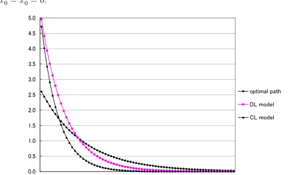
Let ˆxtand x^∗_t denote the gross outstanding local bonds in period t correspond- ing to the MPE and to the optimal solution for the same (x¹₀, x²₀), respectively. One can verify that ˆxt, x^∗_t → ²_r as t → ∞ and that, if x¹₀+ x²₀ < ²_r, ˆxt> x^∗_t for all t since ^β(1+r)_2−β < β(1+r). That is, the gross outstanding local bonds under this MPE are too high compared with the optimal solution. This implies overconsumption during the early periods and underconsumption in the succeeding periods.

2.4 Direct Overcompetitive Distortion

Under the MPE, the intratemporal resource allocation is efficient in the sense that as the consumption of private goods equals that of the local public goods in each

period. However, the outcome of the MPE is inefficient since the intertemporal resource allocation is inefficient.

The reason for the distortion of intertemporal resource allocation may be ex- plained as follows: If the interest rates are constant (r), an economic agent in the private sector who earns one unit of income in every period cannot borrow such that the outstanding amount is more than ¹_r. That is, the outstanding amount is constrained by the present value of future incomes (¹_r). In contrast, in the case of local bonds backed by, or believed to be backed by, the central government, the sum of outstanding local bonds is constrained by the discounted sum of the future income in both regions. In other words, the upper bound of borrowing is com- mon between agents. For example, each agent can borrow even if its outstanding amount is over the discounted sum of the future incomes, as long as the sum of the outstanding amounts is smaller than the discounted sum of the future incomes in both regions. In this case, the agents compete with each other in borrowing. This competition leads to too great a quantity of outstanding local bonds and distorts the intertemporal resource allocation.

The competition is shown in (14). The last term on the right-hand side of (14) represents that the higher the gross lifetime income is, the more each local govern- ment issues bonds. For example, a decrease in x^j₀ causes a corresponding increase in the outstanding local bonds and a reduction in the local tax in region i as a result of the decrease in the gross lifetime income. We call this distortion induced through a common upper bound of borrowing direct overcompetitive distortion.

This borrowing competition is interpreted as the follows: Both local govern- ments all together consume the gross lifetime income. This is because x¹_t+ x²_t ≤ ²_r is equivalent to c¹_t + g_t¹ + c²_t + g_t² ≤ I(x¹_t−1, x²_t−1). By interpreting the gross life- time income as a common resource, this game has the same structure as a social dilemma.

Moreover, provided xⁱ_t−1 and z_tⁱ are given, each resident can attain an arbitrary amount of consumption (cⁱ_t, g_tⁱ) by setting the outstanding local bond (xⁱ_t) and local tax (y_tⁱ) as follows:

xⁱ_t= g_tⁱ+ cⁱ_t− 1 − z_tⁱ+ (1 + r)xⁱ_t−1, yⁱ_t= 1 − cⁱ_t+ z_tⁱ.

In other words, local governments can decide the amount of consumption (cⁱ_t, g_tⁱ) freely, as long as they satisfy c¹_t+ g¹_t + c²_t+ g²_t ≤ I(x¹_t−1, x²_t−1).⁷ Essentially, this is the same structure as the model of Levhari and Mirman (1980).⁸

When the gross lifetime income increases, local governments try to increase the current consumption. For this purpose, each local government raises the net amount of bond issuance and, at the same time, decreases the local tax to achieve an intratemporal balance. By a transformation of equation (15), x¹_t + x²_t − (1 + r)(x¹_t−1 + x²_t−1) = _2−β² (1 − β)I(x¹_t−1, x²_t−1) − 2 follows. This equation together with equation (16) implies the abovementioned characteristics of the MPE. The solution of the planning problem has the same characteristics. However, from

2

2−β > 1, the increase in the net amount of bond issuance in the MPE is greater than that in the planning problem when the gross lifetime income increases. From (11) and (16), the decrease in the local tax in the MPE is less than that in the planning problem when the gross lifetime income increases, since _2−β¹ > ^1−β₂ . The larger amount of government bond issuance causes greater local tax reduction for intratemporal balance.

Efficiency may be improved if the central government commits itself to neglect- ing the redemption of local bonds. Suppose that the central government commits itself to neglecting the redemption of local bonds and that constraint (3) is re- placed by x¹_t ≤ ¹_r, x²_t ≤ ¹_r for arbitrary t ∈ T . The corresponding MPEs consist only of a pair of strategies whose outcomes are efficient, though the outcome does not always maximize social welfare.

3 Infinitely Iterated DL Model

The infinitely iterated DL model (or “DL model” for short) represents the following situation: In each year, local governments decide the outstanding local bonds and local taxes before the central government decides its subsidies to the resident in each region; and this process is repeated over many years.

7For this reason, it is inferred that the local governments’ strategies are not controllable by the central government’s strategies in any subgame perfect equilibrium.

8The consumption in Corollary 1 is the same as that in the MPE of the modified model of Levhari and Mirman (1980).

3.1 Definition of the Game and the Equilibrium

Environment The basic economic environment is the same as that in the pre- vious section except in the stage game that takes place in each period. In each period, the players’ decisions in the stage game are as follows:

(1) Both local governments decide outstanding local bonds xⁱ_t and local taxes y_tⁱ simultaneously. (First move in period t.)

(2) The central government decides subsidies (z_t¹, z_t²) to each resident to satisfy z_t¹+ z_t² = 0. (Second move in period t.)

(3) Private goods consumption cⁱ_t and local public goods supply g_tⁱ are realized, where cⁱ_t and g_tⁱ satisfy (1) and (2), respectively.

Strategy Set Define the sets of histories (H^L_t) up to the first move in period t as follows:

H^L_t ≡







B1 × Q1 if t = 1 Bt× Qt× St−1 if t ∈ T /{1}.

Using this notation and that defined in the previous section, the local governments’ strategy sets A^D1 and A^D2 and the central government’s strategy set A^D0 are defined as follows: For i = 1, 2,

A^Di ≡ ^{((b₁, q₁), (b₂, q₂), · · · ) ∈ Πt∈T _(R^Ht−1

)2^¯

¯

¯ (∀t ∈ T )(∀h ∈ H^t−1) qt(h) + bt(h) − (1 + r)xⁱ_t−1 ≥ 0 where

h = ((x¹₀, · · · , x¹_t−1), (x²₀, · · · , x²_t−1), yt−1, zt−1)^}, A^D0 ≡ ^{((s¹₁, s²₁), (s¹₂, s²₂), · · · ) ∈ Πt∈T_(R^H

L t₎²

¯

¯

¯ (∀t ∈ T )(∀h ∈ ^H

L t⁾

(∀i ∈ {1, 2}) 1 − yⁱ_t+ sⁱ_t(h) ≥ 0, s¹_t(h) + s²_t(h) = 0 where h = (xt, ((y₁¹, · · · , y_t¹), (y₁², · · · , y_t²)), zt−1)^}.

For given ((s¹₁, s²₁), (s¹₂, s₂²), · · · ) ∈ A^D0, sⁱ_{t ∈ R}^HLt represents a function that assigns subsidies to the resident in region i in period t. In period t, the central government decides subsidies depending on the history up to period (t − 1) and also based